Abstract
The barotropic sea level difference (SLD) across the Korea/Tsushima Strait (KTS) is considered an index of the volume transport into the East/Japan Sea. This study investigates the interannual variability of the barotropic SLD (the KTS inflow) from 1985 to 2017 and its relationship to upper-ocean (<300 m) current variability in the western North Pacific. An increase in the KTS inflow is associated with a weakening of the Kuroshio current through the Tokara Strait and upper-ocean cooling in the North Pacific Subtropical Gyre, characteristic of a La Niña-like state. Diagnostic analysis reveals that the KTS inflow variability is linked to at least two statistically distinct and concurrent modes of oceanic variability. The first mode is tied to the El Niño–Southern Oscillation through large-scale changes in the Kuroshio system. The second mode, which is linearly uncorrelated with the first, is associated with regional eddy kinetic energy variability in the western North Pacific. The identification of these parallel pathways suggests a complex regulatory system for the KTS inflow. This study provides a new framework for understanding the multi-faceted connection between the KTS and upstream oceanic processes, with implications for the predictability of the ocean environmental conditions in the East/Japan Sea.
1. Introduction
The Kuroshio, a western boundary current in the North Pacific, flows northward after bifurcating from the North Equatorial Current (NEC), passes to the east of the Luzon Strait and Taiwan, and enters the East China Sea (ECS). The main path of the Kuroshio branches to the southwest of Kyushu (Figure 1a), with approximately 11% intruding into the shelf region of the ECS and flowing into the East/Japan Sea (EJS) through the Korea/Tsushima Strait (KTS) [1,2,3,4]. The inflow through the KTS transports subtropical buoyant water from the western North Pacific to the EJS, governing upper-ocean circulation and climate variability in the EJS [4,5,6,7]. It is important to investigate how the inflow through the KTS varies and what regulates this variability in order to understand ocean environmental variability in the EJS [8,9,10].

Figure 1.
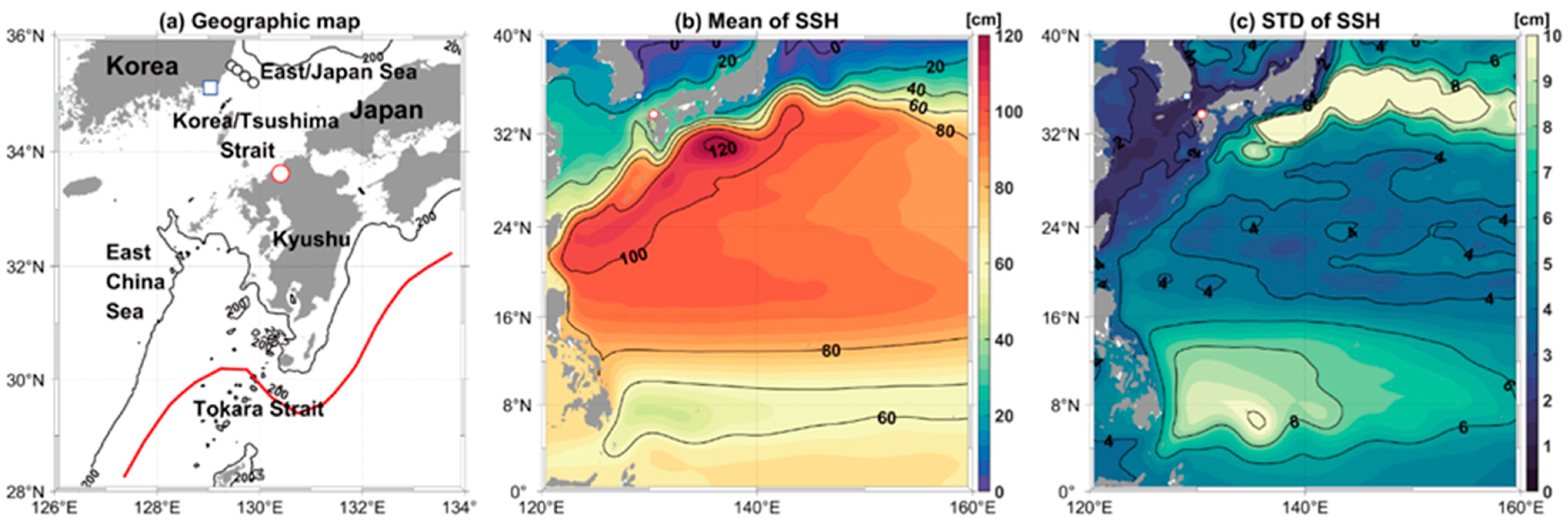
(a) The map around the Korea/Tsushima Strait with 200 m isobaths in black contour. The thick red line denotes the mean Kuroshio pathway defined by the 100 cm contour of the mean sea surface height (SSH) from the SODA 3.4.2 dataset for 1985–2017. The black open dots denote hydrographic stations Nos. 1–4 (from west to east) along line 208 of the Korea Oceanographic Data Center. (b) The mean SSH for 1985–2017 in the western North Pacific (color shading interval: 5 cm). (c) The standard deviation of the 24-month low-pass-filtered SSH for 1985–2017 (color shading interval: 0.5 cm). The blue square and red dot denote the location of Busan (Republic of Korea) and Hakata (Japan), respectively.
The inflow through the KTS is known to exhibit an inverse relationship with the main Kuroshio current through the Tokara Strait [1,11]. The inflow exhibits significant seasonal variability, with maximums in summer and minimums in winter, associated with the seasonal cycles of the main Kuroshio and the Ekman transport in the ECS induced by the East Asian Monsoon [12,13,14]. The long-term (>seasonal) variability of inflow through the KTS is reported to be influenced by the large-scale wind-stress curl (WSC) over the North Pacific associated with the Pacific Decadal Oscillation and the Arctic Oscillation, among others [7,9,10,15]. However, the physical mechanism of how the upstream Kuroshio current (from the Luzon Strait to the northern ECS in this study) influences the interannual variability of the inflow through the KTS has remained an open question [10].
The strength of the upstream Kuroshio current is related to changes in the North Pacific Subtropical Gyre (NPSG) and the bifurcation latitude of the NEC [16,17,18,19]. Figure 1b,c depict the mean and standard deviations (STDs) of the two-year low-pass-filtered sea surface height (SSH) for 1985–2017 in the western North Pacific. The mean SSH illustrates the NPSG (orange to red) and the bifurcation latitude of the NEC along approximately 13.5° N [20,21]. Strong SSH variability exists between 7° and 15° N, which is due, in part, to the meridional shifts in the NPSG and the NEC, which are connected to the large-scale WSC variability over the North Pacific [20,22]. Previous studies have explained the meridional shift in the NPSG and NEC during El Niño–Southern Oscillation (ENSO) years; the NPSG and NEC shift northward during El Niño years, while they shift southward during La Niña years [19,23,24,25].
The WSC over the western North Pacific is also related to the strength of the Kuroshio current through eddy activity in the western North Pacific [26,27]. Recent studies suggest that the eddy kinetic energy (EKE) in the western North Pacific increases as a consequence of an increase in baroclinic instability between the NEC and the Subtropical Counter Current (STCC) driven by the WSC variability over the North Pacific [22,25,26,28]. Eddies frequently occur in the region between the NEC and the STCC and propagate towards the Luzon Strait or southeast of Taiwan, regulating the upstream Kuroshio and the Kuroshio in the ECS [29,30,31]. Thus, previous studies imply a possible connection between the inflow through the KTS and EKE variability in the western North Pacific, considering the inverse relationship between the volume transport through the KTS and the main Kuroshio current.
In this study, the barotropic sea level difference (SLD) between Busan (Republic of Korea) and Hakata (Japan) is used as an index for the volume transport through the KTS based on its geostrophic relationship established in previous studies [10,32]. The interannual variability of the barotropic SLD across the KTS is investigated in relation to upper-ocean variability in the western North Pacific. To examine interannual variability, the analysis begins by characterizing the dominant seasonal cycle before moving on to the main focus of this study. While previous studies have often attributed KTS inflow variability to a single dominant factor, such as large-scale climate modes or regional Kuroshio dynamics, this study adopts a more comprehensive diagnostic framework. It concurrently investigates both ENSO-related processes and ENSO-irrelevant oceanic variability, focusing particularly on the potential role of eddy kinetic energy (EKE) in the western North Pacific. The primary goal is not only to identify potential drivers but also to explore whether multiple, distinct forcing mechanisms operate in parallel. The identification of such co-existing and potentially independent pathways would suggest a more complex regulatory system for KTS inflow than previously understood. Section 2 describes the data and methods. Section 3 examines the interannual variability of the KTS inflow and its connection to the ocean environment. Section 4 provides a discussion and summary.
2. Data and Methods
2.1. Data
To estimate volume transport through the KTS, monthly tide gauge data from Busan (Republic of Korea) and Hakata (Japan) were used for 1985–2017, provided by the Permanent Service for Mean Sea Level (PSMSL; https://www.psmsl.org/data/obtaining/; accessed on 2 March 2024) [33]. The line connecting the two locations is almost perpendicular to the major axis of the KTS (Figure 1) [10,32,34]. Bimonthly observed temperature and salinity data along Line 208 (the black dots in Figure 1a) from the Korea Oceanographic Data Center (KODC; https://nifs.go.kr/kodc/soo_list.kodc; accessed on 20 May 2024) were used to exclude the baroclinic SLD across the KTS for 1984–2018, as it does not induce volume transport [32,34]. Hydrographic observation data from the KODC are available only in the western channel of the KTS (Station 1–4) due to the 1998 Korea–Japan Fisheries Agreement on Exclusive Economic Zones. The baroclinicity of the flow is dominant in the western channel rather than the eastern channel due to the Korea Strait Bottom Cold Water (<10 °C) in the western channel of the KTS [2,32,35]. Therefore, the baroclinic SLD across the KTS is mostly determined using limited hydrographic data and only in the western channel of the KTS [32].
To understand upper-ocean environmental variability related to changes in volume transport through the KTS, monthly SSH, temperature, and current velocity data at depths of 5–300 m were obtained from Simple Ocean Data Assimilation (SODA; https://www.soda.umd.edu; accessed on 11 April 2024) version 3.4.2 for 1985–2017. These were employed with a spatial resolution of 0.5°. The SODA 3.4.2 uses the ERA-Interim reanalysis dataset for atmospheric forcing, which is accessible from the European Centre for Medium-Range Weather Forecasts (ECMWF) [36]. To examine eddy-related oceanic processes possibly connected to inflow through the KTS, monthly EKE was calculated using the geostrophic velocity anomalies from the Copernicus Marine and Environment Monitoring Service (CMEMS; http://marine.copernicus.eu; accessed on 12 March 2024) for 1993–2017 with a spatial resolution of 0.25° [37]. Note that the EKE dataset is available only for 1993–2017, which is a shorter period than other datasets due to the limited availability of satellite altimetry data. Consequently, all regression analyses involving EKE were conducted for this 1993–2017 period, while analyses for all other variables utilized the full 1985–2017 period.
The ERA 5 monthly averaged 10 m wind velocity, and its WSC were used for the same period with a horizontal resolution of 0.25°, as provided by the ECMWF (https://www.ecmwf.int/en/forecasts/dataset/ecmwf-reanalysis-v5; accessed on 12 March 2024) [38]. Also, monthly averaged Optimum Interpolation SST (OISST) version 2.1 (https://downloads.psl.noaa.gov/Datasets/noaa.oisst.v2.highres/; accessed on 21 March 2024) with a spatial resolution of 0.25° was also used. The OISST dataset is made up of SST recordings from a variety of sources, including satellites, vessels, and buoys [39]. Except for the monthly tide gauge data, all other datasets were investigated at the following three different spatial domains: (1) around the KTS (28–36° N, 126–134° E), (2) the western North Pacific (16–32° N, 120–132° E), and (3) the wider domain of the western North Pacific (6–36° N, 120–136° E). The wider domain was chosen to encompass the upstream Kuroshio system, including the NEC and STCC, which are the primary large-scale features considered to influence the KTS inflow.
2.2. The Calculation of the Barotropic Sea Level Difference Across the KTS
The SLD (Hakata–Busan) can be used as an index of volume transport through the KTS under a geostrophic balance after removing its baroclinic part [10,32,40,41]. To remove the baroclinic SLD () from the SLD, the difference between geopotential heights (D) and depth-averaged geopotential heights () was calculated using hydrographic data from stations 4 (east) and 1 (west) along the KODC line 208. Their baroclinic SLD () was calculated as shown in Equation (1) [32,42]:
where g denotes gravitational acceleration. The cubic-spline method was applied to interpolate the bimonthly baroclinic SLD to monthly values for 1985–2017. Finally, the barotropic SLD was determined by subtracting the baroclinic SLD from the SLD. This method, based on established previous studies [32,42], assumes a linear relationship by utilizing the baroclinic correction based on the available hydrographic data. This assumption is further discussed as a limitation in Section 4.1.
2.3. Cyclostationary Empirical Orthogonal Function and Regression Analysis
The cyclostationary empirical orthogonal function (CSEOF) analysis [43,44] was applied to the one-dimensional time series of the barotropic SLD across the KTS, the two-dimensional time series (SSH, 10 m wind velocity, WSC, SST, and EKE), and each layer of the three-dimensional time series (temperature, salinity, and current velocity). The CSEOF analysis has been a useful statistical analysis tool for investigating geophysical environmental variables, such as air–sea interactions and fish stock, among others [7,45,46]. No prior detrending was applied to the time series, as the CSEOF analysis can effectively separate long-term trends from oscillatory modes [45]. In this study, the CSEOF technique was used to extract the interannual variabilities of the barotropic SLD and each environmental variable for the three different spatial domains, as described in Section 2.1, around the KTS, the western North Pacific, and the wider domain of the western North Pacific.
In the CSEOF, the two-dimensional time series or each vertical layer of the three-dimensional variables were decomposed as cyclostationary loading vectors (CSLVs), and their corresponding principal component (PC) time series, as shown in Equation (2):
where , , and denote the mode number, space, and time, respectively. The physical evolution of variables is represented by CSLVs, and the nth mode of CSLVs is expressed with a periodicity of d, which is set to 12 months in this study, as shown in Equation (3):
Thus, each mode of the CSLVs is made up of 12 monthly spatial patterns and its corresponding PC time series, , illustrates the long-term temporal variation in the nth mode of physical evolution. Thus, the CSEOF method with a 12-month periodicity inherently separates the annually repeated cycles (i.e., the seasonal cycle) from the non-seasonal long-term variations (i.e., interannual variability) represented in the subsequent modes. Typically, the first mode represents the seasonal cycle, while higher modes capture interannual to decadal variability. It is important to note that CSLVs are perpendicular to each other and that each of the PC time series is statistically independent.
The one-dimensional time series variable representing the barotropic SLD in this study was decomposed, as shown in Equation (4):
where and denote the mode number and time, respectively, which is the same as Equation (2). Similarly to the multi-dimensional variables, also contains 12 monthly variations, and its corresponding PC time series, , illustrates the temporal variation in the nth mode of physical variation. Then, the interannual barotropic SLD mode, , was selected considering the nth mode of the annual variation in and the periodicity of the PC time series . The details of selecting the interannual barotropic SLD mode are described in Section 3.1.
To understand the environmental variability related to the interannual barotropic SLD across the KTS, a regression analysis was conducted for each variable targeting the interannual variability of the barotropic SLD across the KTS, , as in Equation (5):
where denotes the mode number, is the regression coefficient, and is the PC time series of each multi-dimensional time series variable. The regressed and reconstructed CSLVs, , represent the environmental variabilities related to the interannual variability of the barotropic SLD and were acquired through the regression coefficients, , as shown in Equation (6):
where the is composed of 12 monthly spatial patterns for each variable at each level. The thus displays consistent spatio-temporal variability with the interannual variability of the barotropic SLD, . To highlight the interannual variability, each is presented as the annual mean of the spatial patterns. The regression was carried out over the period of the barotropic SLD, 1985–2017 (1993–2017 for the EKE). The R-squared values for the regression of temperature and current velocity are shown at each depth in Supplementary Figure S1.
3. Results
3.1. Sea Level Differences Across the KTS
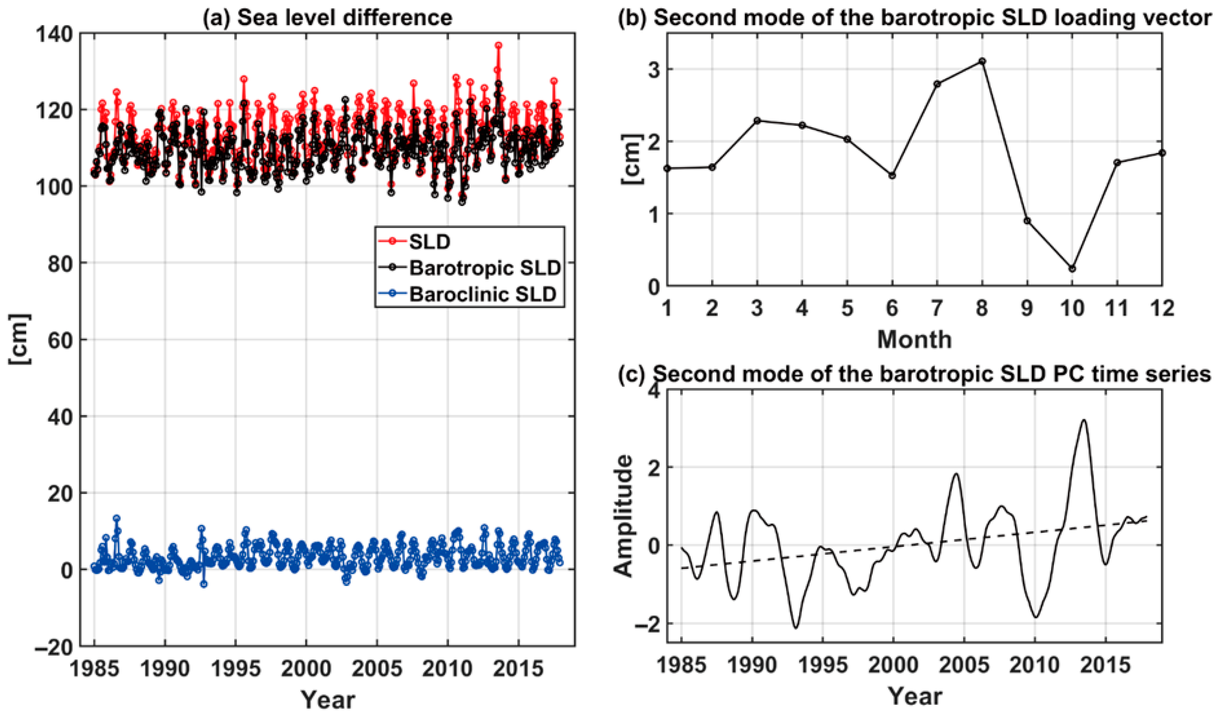
Figure 2a depicts the SLD across the KTS with its barotropic and baroclinic components for 1985–2017. The barotropic SLD has a strong correlation with the volume transport through the KTS observed from vessel-mounted Acoustic Doppler Current Profilers on the ferryboat Camellia between Busan and Hakata [47] (r = 0.69, p < 0.01 during January 1997–February 2007; see Supplementary Figure S2). Based on this long-term linear relationship, this study considers barotropic SLD as an index of the inflow through the KTS [32,47]. Figure 2b,c illustrate the monthly variation (loading vector) and corresponding PC time series of the second mode of barotropic SLD across the KTS from 1985 to 2017. The first mode of the barotropic SLD exhibits a seasonal cycle (Supplementary Figure S3). Aside from the seasonal cycle, the second mode explains approximately 38% of the total variance. The loading vector exhibits a positive SLD anomaly throughout the year, reaching its maximum in late summer (August) and minimum in autumn (October) (Figure 2b). Its corresponding PC time series displays interannual variability with a periodicity of about 4 years. The loading vector and corresponding PC time series in Figure 2 suggest that the second mode of the barotropic SLD represents the interannual variability of the barotropic SLD. During 1985–2017, the interannual barotropic SLD increased at a rate of 0.67 mm/year, accounting for approximately 23% of the interannual standard deviation. This long-term increasing trend is consistent with a study which showed that the inflow through the KTS has increased in recent decades [10].

Figure 2.
(a) Sea level difference (SLD) across the Korea/Tsushima Strait for 1985–2017 and its barotropic and baroclinic components. (b) The monthly cyclostationary loading vector of the second mode of the barotropic SLD. (c) The principal component (PC) time series of the second mode of the barotropic SLD for 1985–2017. The dashed line denotes the linear trend of the PC time series. Note that (b) illustrates the characteristic annual pattern of the anomaly associated with this interannual mode, not a time series of events.
3.2. Inflow Through the KTS and Ocean Environment Around the KTS
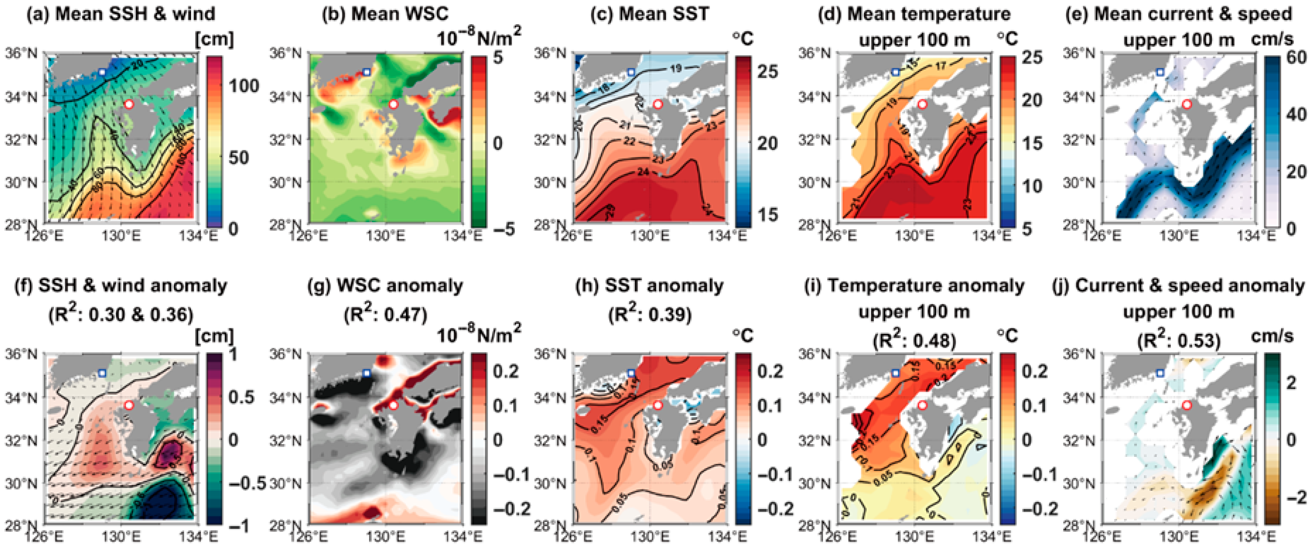
Figure 3 shows the mean and regressed anomalies of environmental variables around the KTS for 1985–2017, targeting the interannual variability of barotropic SLD in Figure 2. In Figure 3f, there is a positive SSH anomaly along the western coast of Kyushu. The positive SSH anomaly on the eastern side of the KTS indicates an increase in the inflow through the KTS based on a geostrophic balance, demonstrating physical consistency with the target mode of regression. In the Tokara Strait, positive and negative SSH anomalies are observed onshore and offshore, respectively, representing a deceleration of the Kuroshio current. Northeasterly wind anomalies suggest the enhanced onshore Ekman transport of the Kuroshio current towards the KTS region [14,48]. SST and upper-ocean temperature anomalies exhibit an overall warming around the KTS, suggesting a relationship with an increase in the inflow through the KTS on the interannual time scale. It is notable that the warming in the upper 100 m is significant only around the KTS and northern ECS, excluding the region of the main path of the Kuroshio current in the Tokara Strait. The regressions for SSH, SST, and temperature are statistically significant (p < 0.05).
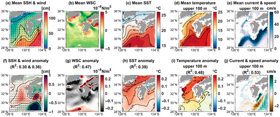
Figure 3.
(Top) The mean environmental variables around the Korea/Tsushima Strait for 1985–2017: (a) sea surface height (SSH; color shading and contours with an interval of 20 cm) and the wind (vector); (b) wind-stress curl (WSC; color shading interval: 0.5 10−8 N/m2); (c) sea surface temperature (SST; color shading and contours with an interval of 1 °C); (d) the upper 100 m depth-averaged temperature (color shading and contours with an interval of 2 °C); and (e) the upper 100 m depth-averaged currents (vector) and speed. (Bottom) Regression anomalies onto the second mode of the barotropic SLD across the Korea/Tsushima Strait: (f) SSH (contour interval: 0.5 cm) and wind (vector); (g) WSC; (h) SST (contour interval: 0.05 °C); (i) upper 100 m depth-averaged temperature (contour interval: 0.05 °C); and (j) upper 100 m depth-averaged currents (vector) and speed. The R-squared values of each regression are presented in parentheses with statistical significance at the p < 0.05 level. The blue square and red dot denote the location of Busan (the Republic of Korea) and Hakata (Japan), respectively.
The current anomalies in the upper 100 m exhibit an increase in the current anomaly over the shelf region near the KTS, suggesting an increase in the inflow through the KTS. In the Tokara Strait, the current anomalies illustrate a deceleration in the Kuroshio current along the main pathway, which is physically consistent with the SSH anomalies. In addition, there is a statistically significant negative relationship between the annually averaged interannual barotropic SLD across the KTS and the annual mean observed volume transport through the Tokara Strait reported by Liu et al. [49] (r = −0.53 during 1998–2013, p < 0.05). The regression results and correlation coefficient suggest that when the inflow through the KTS increases, the Kuroshio decelerates in the Tokara Strait on the interannual time scale. This inverse relationship between the inflow through the KTS and the Kuroshio current is consistent with previous studies [1,11].
3.3. The Inflow Through the KTS and Ocean Environment in the Wider Domain of the Western North Pacific
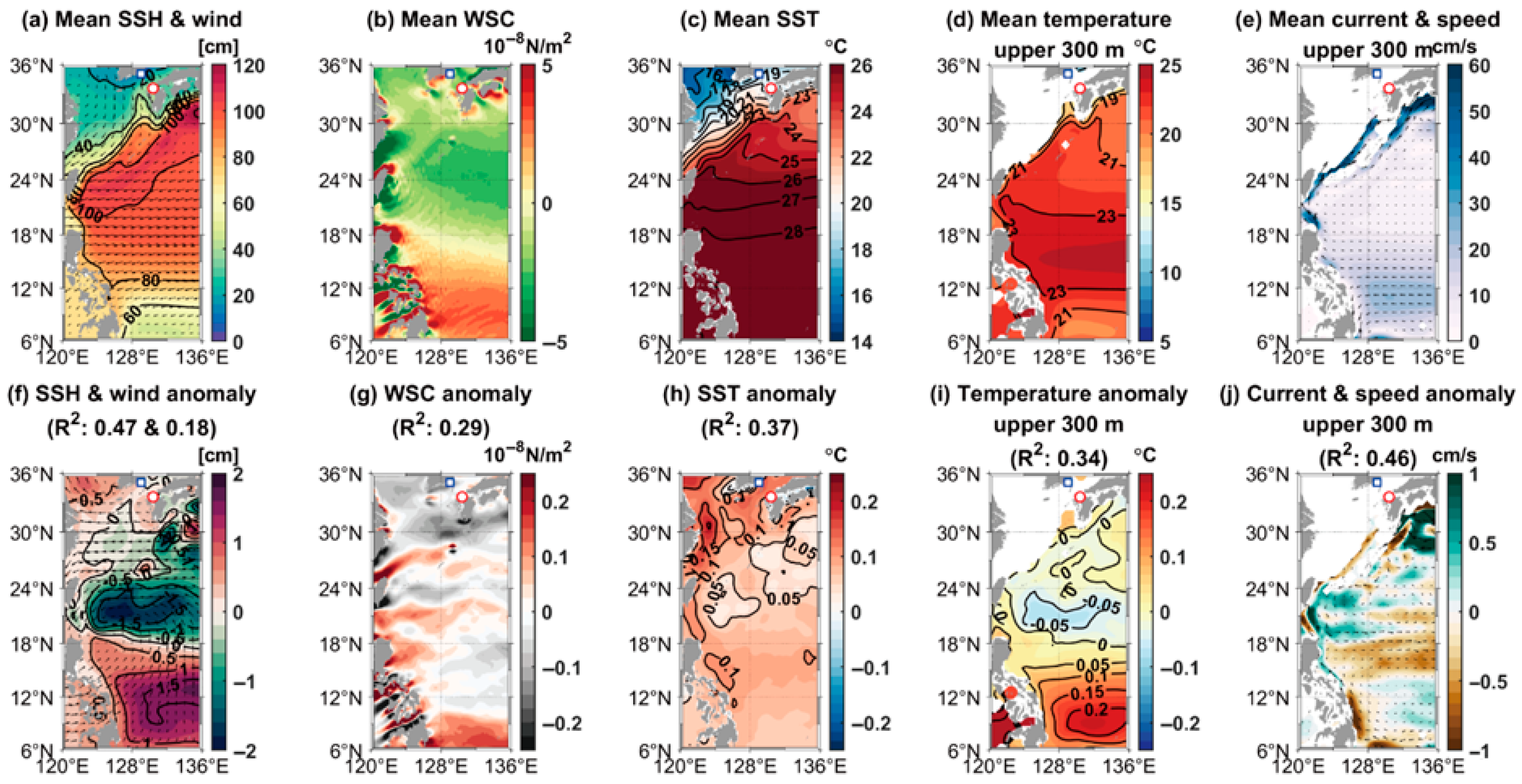
Figure 4 shows the means and regressed anomalies of environmental variables in the wider domain of the western North Pacific for 1985–2017, targeting the interannual variability of barotropic SLD in Figure 2. The SSH displays a negative anomaly to the north of 18° N, indicating a weakening of the Kuroshio current. The cyclonic wind anomalies are observed over the latitudinal band of the NEC and STCC, between 12° and 24° N, but the wind and WSC anomalies exhibit relatively insignificant R-squared values. The insignificant R-squared values indicate that the large-scale atmospheric variability in the western North Pacific is not directly connected with the interannual variability of the inflow through the KTS.

Figure 4.
(Top) The mean environmental variables in the western North Pacific for 1985–2017: (a) sea surface height (SSH) and the wind (vector); (b) wind-stress curl (WSC; color shading interval: 0.5 10−8 N/m2); (c) sea surface temperature (SST); (d) the upper 300 m depth-averaged temperature; and (e) the upper 300 m depth-averaged currents (vector) and speed. (Bottom) Regression anomalies onto the second mode of the barotropic SLD across the Korea/Tsushima Strait: (f) SSH (contour) and wind (vector); (g) WSC; (h) SST; (i) upper 300 m depth-averaged temperature; and (j) upper 300 m depth-averaged currents (vector) and speed. The R-squared values of each regression are presented in parentheses with statistical significance at the p < 0.05 level. The blue square and red dot denote the location of Busan (the Republic of Korea) and Hakata (Japan), respectively.
The SST anomaly shows overall warming around the KTS and in the shelf region of the ECS but not significantly along the main pathway of the Kuroshio current and in the NPSG region. The temperature anomaly of the upper 300 m illustrates cooling in the NPSG (north of 18° N). This cooling would be associated with a weakening of the Kuroshio current. Indeed, the upper 300 m current anomalies exhibit a deceleration in the Kuroshio current in the ECS. The longitudinally averaged (124–126° E) meridional current velocity anomaly in the upper 300 m suggests equatorward shifts in the NPSG and the bifurcation latitude of the NEC (see Supplementary Figure S4). A similar ocean condition emerges during the La Niña years [19,26,50,51]. Therefore, the regressed anomalies in Figure 4 exhibit a La Niña-like ocean environment, and these regression results suggest a link between inflow through the KTS and the ENSO.
3.4. The Inflow Through the KTS and Upper-Ocean Currents in the Western North Pacific
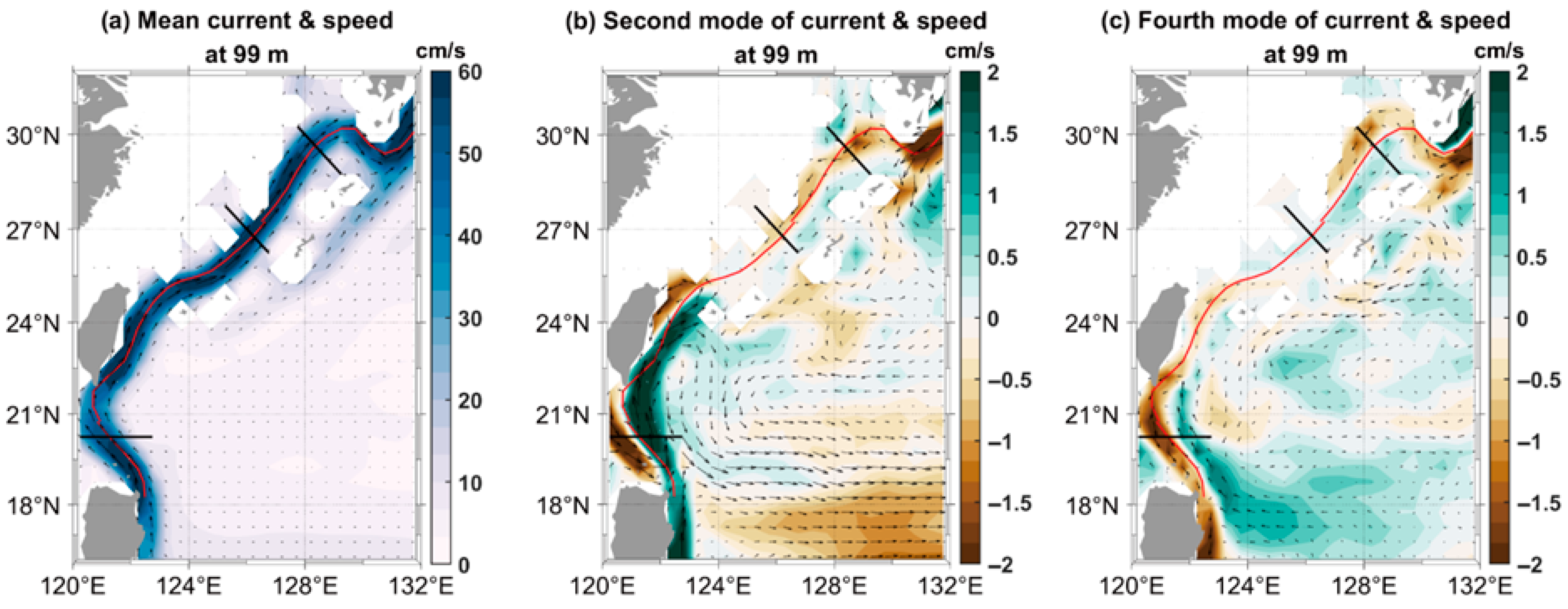
Figure 5 illustrates the mean and variability of the current at a depth of 99 m in the western North Pacific. The yearly averaged loading vectors of the second and fourth modes are shown in Figure 5b,c, respectively. Their corresponding PC time series can be found in Supplementary Figure S5. The second (~8% of the total variance) and fourth (~6% of the total variance) modes were selected based on their relatively higher correlation coefficients with the interannual variability of the barotropic SLD (r = 0.41, p < 0.05 and r = 0.40, p < 0.05, respectively) compared to other modes. The positive correlations indicate that the anomalies shown in Figure 5b,c are related to the increase in the inflow throughout the KTS. The vertical sections of mean speed with regressed anomalies are illustrated in Supplementary Figure S6 for the Luzon Strait, the Kuroshio current in the ECS, and the southwest of Kyushu. Among the modes representing interannual variability, the second and fourth modes were chosen for detailed analysis as they exhibited the most prominent and statistically significant correlations with the interannual barotropic SLD.

Figure 5.
(a) The mean currents (vector) and speed (color shading) at 99 m from the Luzon Strait to the south of Kyushu for 1985–2017. (b) The second mode of current (vector) and speed (color shading interval: 0.2 cm/s) anomalies. (c) The same as (b), but for the fourth mode. Red lines illustrate the Kuroshio mean pathway for 1985–2017 (defined by 100 cm contours in the SSH), and black thick lines indicate the locations of vertical sections in the Luzon Strait, Kuroshio in the ECS, and the southwest of Kyushu in Supplementary Figure S6.
The second mode of current variability at 99 m depicts a weakening of the NEC and an offshore shift in the upstream Kuroshio current (Figure 5b and Supplementary Figure S6). The second mode also shows an overall weakening of the Kuroshio in the ECS and in the Tokara Strait, along with a meandering to the southwest of Kyushu, which could be related to the positive correlation with the interannual variability of the barotropic SLD (an increase in the inflow through the KTS). The PC time series of the second mode exhibits a statistically significant correlation with the ENSO (Supplementary Figure S7: r = −0.53 and p < 0.01 with a 2-year low-pass-filtered Niño 3.4 index from 1985 to 2017). The fourth mode, however, illustrates relatively weak anomalies in the lower latitudes and the upstream Kuroshio region (Figure 5c and Supplementary Figure S6). The fourth mode displays an offshore shift in the Kuroshio current in the ECS but an onshore shift in the Kuroshio current in the Tokara Strait. The correlation between the fourth mode and the ENSO is negligible. Thus, it is suggested that the two modes of the current variability associated with the interannual variability of the barotropic SLD exhibit different characteristics: ENSO-related characteristics for the second mode and ENSO-irrelevant characteristics for the fourth mode.
4. Discussion
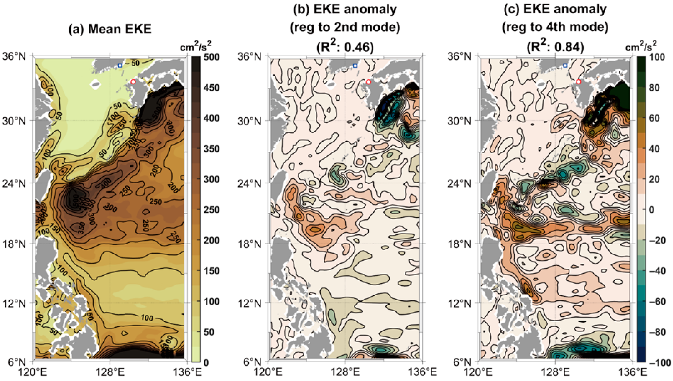
The ENSO-related and ENSO-irrelevant modes of current variability depicted in Figure 5 could be related to changes in the inflow through the KTS via different processes of ocean environmental variability. Figure 6 depicts the mean EKE and regressed EKE anomalies for the second and fourth modes of current variability at 99 m from 1993 to 2017, as displayed in Figure 5. Both of the regressed anomalies exhibit an increase in the EKE to the east and southeast of Taiwan; however, the amplitude is greater for the regression targeting the fourth mode (ENSO-irrelevant mode). Specifically, the EKE anomaly that regressed onto the ENSO-irrelevant mode (Figure 6c) showed notable peaks along 21° N, whereas the anomaly that regressed onto the ENSO-related mode (Figure 6b) was weaker in this region. The higher R-squared value of the regression also suggests that the ENSO-irrelevant mode of current variability is strongly associated with the EKE variability. The EKE anomaly, when regressed onto the ENSO-irrelevant mode, exhibits strong positive anomalies, particularly along 21° N, possibly due to an enhancement in baroclinic instability between the NEC and the STCC (see Figure 5c and the third column in Figure 6) [22,52]. In addition, strong positive anomalies of EKE are observed to the east of the Tokara Strait. Understanding how these anomalies influence the interannual variability of the inflow throughout the KTS requires more in-depth analysis, which is beyond the scope of this study.
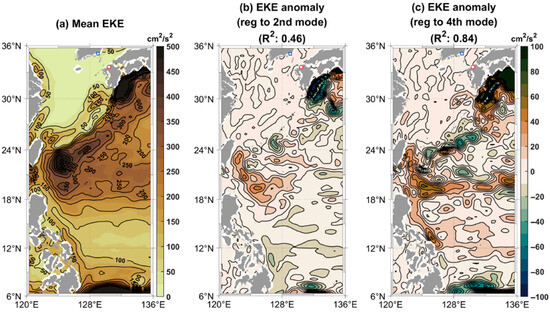
Figure 6.
(a) The mean eddy kinetic energy (EKE) during 1993–2017 (contour interval: 25 cm2/s2). (b) The regressed EKE anomaly (contour interval: 10 cm2/s2) derived from the second mode. (c) The same as (b), but for the fourth mode (ENSO-irrelevant mode) of 99 m current anomalies. The R-squared values for each regression are displayed in the titles within parentheses. These regressions were performed for the 1993–2017 period. The blue square and red dot denote the location of Busan (Republic of Korea) and Hakata (Japan), respectively.
This study investigated the interannual variability of the barotropic SLD across the KTS and its relationship with upper-ocean dynamics in the western North Pacific. The results reveal a system of greater complexity than often portrayed, where the KTS inflow is associated with multiple, physically distinct modes of ocean variability. A key finding is the identification of at least two separate pathways influencing KTS inflow on interannual timescales. The analysis distinguished an ENSO-related mode of current variability from an ENSO-irrelevant mode. The former is characterized by large-scale adjustments in the Kuroshio current and NPSG, which is consistent with known responses to ENSO forcing. The latter, however, appears statistically independent from ENSO and shows a stronger association with regional EKE variability, particularly in the vicinity of the NEC-STCC system and east of Taiwan.
The statistical orthogonality of these modes, a feature of the CSEOF analysis, indicates that they represent linearly uncorrelated processes within the analyzed period. This suggests that the KTS inflow is modulated by the superposition of influences from at least two statistically separable pathways: one linked to large-scale climate patterns and another to relatively localized, internal ocean dynamics. It is important to note that statistical separability does not preclude the possibility of a more complex, underlying, non-linear relationship or time-lagged connection between ENSO and regional EKE generation. For instance, ENSO could precondition the background oceanic state over several years, influencing the environment where eddies form. Exploring such complex interactions is beyond the scope of this diagnostic study, but the clear separation of their contemporaneous, linear expressions is a key finding that highlights the multi-faceted nature of these forcing mechanisms.
Another notable aspect of the findings is the modest magnitude of the individual correlations. While statistically significant, neither the ENSO-related mode nor the EKE-related mode individually explains a dominant portion of the total variance in KTS inflow. Rather than indicating a weakness in relationships, this finding suggests that a complete understanding of KTS inflow variability cannot be achieved by focusing on a single driver. The system appears to be inherently complex, with its total variability arising from a combination of these identified factors and potentially others not resolved in this study, such as local atmospheric forcing mechanisms or shelf–ocean interactions. The linkage between the ENSO-irrelevant mode and EKE (Figure 6) suggests the importance of mesoscale processes. The enhanced EKE near the NEC-STCC region, a known site of baroclinic instability [22,52], could generate eddies that propagate westward, ultimately influencing the Kuroshio’s pathway and its branching into the ECS. The detailed mechanisms of this teleconnection, however, remain a subject for future investigation. This diagnostic study serves to highlight these distinct statistical linkages, thereby providing a foundation and a clear motivation for future process-based modeling studies.
Limitations and Future Directions
This study presents statistical linkages between KTS inflow and large-scale ocean variability on the interannual time scale, but it is subject to several limitations that should be acknowledged. First, the analysis relies on certain assumptions and datasets that have constraints. The calculation of the barotropic SLD, despite following established methods, assumes a simplified relationship based on limited hydrographic data from the western channel of the KTS and does not account for potential non-linearities or variability in the eastern channel. Second, there is a temporal mismatch between the EKE dataset (1993–2017) and other datasets (1985–2017), which limits the period over which their relationship can be analyzed. Third, some of the reported correlation coefficients are statistically significant but modest in magnitude (e.g., r ≈ 0.4). As discussed, this may reflect the true complexity of the system, where multiple factors exert partial influence instead of a single dominant control. However, it also highlights that a substantial portion of the variance remains unexplained by the large-scale drivers considered here. The robustness of these modest correlations could also be influenced by the relatively short record length (~30 years) and potential autocorrelation in the time series.
Furthermore, this study is primarily diagnostic and correlational in nature. While it successfully identifies and separates statistically distinct associations between KTS inflow, ENSO, and EKE, it does not resolve the underlying physical dynamics. For instance, the precise mechanisms by which ENSO-induced wind forcing propagates through the ocean system—such as via equatorial Kelvin or Rossby waves—to affect KTS inflow or how EKE anomalies directly modulate the Kuroshio pathway and its branching remain open questions. While our findings regarding an inverse relationship between KTS and Tokara Strait transport are consistent with some studies [1,11], reconciling them with the findings of all previous works, which may focus on different timescales or mechanisms [49], requires more detailed analysis. These limitations do not diminish the diagnostic findings but rather sharpen the focus for future research. A deeper understanding would benefit from the use of high-resolution, eddy-resolving ocean models to conduct process-based studies. Such models could be used to perform sensitivity experiments to untangle the roles of wind forcing, baroclinic instability, and remote wave propagation, thereby providing a more comprehensive dynamical framework for the variability of inflow in the KTS.
5. Summary and Concluding Remarks
In summary, this study examines the interannual variability of barotropic inflow through the KTS from 1985 to 2017. The analysis provides evidence for a multi-faceted control system, challenging the notion of a single dominant driver. The main conclusions are as follows:
- 1.
- An increase in the KTS inflow is associated with a La Niña-like state in the western North Pacific, involving a weaker Kuroshio current and an equatorward shift in the NPSG.
- 2.
- The variability in KTS inflow is linked to at least two statistically distinct modes of upper-ocean current variability. These modes are linearly uncorrelated in the contemporaneous analysis, with one clearly tied to ENSO and the other associated with relatively regional EKE, suggesting the presence of multiple forcing pathways.
- 3.
- The identification of these parallel pathways suggests that both large-scale climate forcing and internal oceanic dynamics contribute to modulating the KTS inflow. The modest explanatory power of each individual pathway underscores the inherent complexity of the system.
The principal contribution of this work lies in providing a more nuanced perspective on the regulation of KTS inflow, which has direct implications for future predictability studies. By demonstrating that this system is influenced by at least two statistically distinct and concurrent pathways, this study challenges prediction models that rely on a single predictor, such as an ENSO index alone. The results suggest that a portion of the prediction error in such models may stem from the unmodeled, ENSO-irrelevant variability driven by internal ocean dynamics like EKE. Therefore, improving the predictability of KTS inflow, and by extension, the ocean environment in the EJS, may require the development of new frameworks that can incorporate both large-scale climate signals and metrics of regional mesoscale activity. While this finding underscores the challenge of prediction, it provides a crucial diagnostic insight into sources of variability, laying the groundwork for more robust and physically complete prediction systems.
Supplementary Materials
The following supporting information can be downloaded at https://www.mdpi.com/article/10.3390/cli13070144/s1, Figure S1: R-squared values for the multiple linear regression of the interannual barotropic SLD onto the principal components of (a) upper-ocean temperature and (b) currents at each depth level. Figure S2: (a) Monthly barotropic SLD across the KTS from Jan 1997–Feb 2007. (b) Observed volume transport through the KTS from Fukudome et al., (2010) [47] for the same period as in (a). (c) Normalized barotropic SLD and volume transport for the same period as in (b). Figure S3: (a) Monthly climatological mean SLD and calculated barotropic SLD across the KTS for 1985–2017 with their standard deviations. (b) The monthly cyclostationary loading vector of the first mode of the barotropic SLD. (c) The PC time series of the first mode of the barotropic SLD for 1985–2017. Figure S4: (left) Mean meridional current velocity longitudinally averaged from 124°E to 126°E for 1985–2017. (right) Regressed anomalies of meridional current velocity longitudinally averaged from 124°E to 126°E regressed onto the second mode of the barotropic SLD across the KTS. Figure S5: The PC time series of the interannual barotropic SLD (the second mode) (black), the second mode (red), and the fourth mode of current 99 m depth in the western North Pacific (blue) for 1985–2017. Figure S6: Vertical Sections of upper 300 m depth speed in the Luzon Strait, the East China Sea, and the Southwest of Kyushu. (top) Mean speed for 1985–2017. (middle) Regressed upper 300 m depth speed anomaly onto the second mode of currents at 99 m depth in the western North Pacific. (bottom) Same as (middle), but for the fourth mode of currents. Figure S7: (a) The second mode of zonal current velocity anomaly in the equatorial Pacific during 1985–2017. (b) Regressed zonal current velocity anomaly onto the second mode of currents at 99 m depth in the western North Pacific. (c) The PC time series of the second mode of currents at 99 m depth with 2-year low-pass filtered Niño 3.4 index.
Author Contributions
Conceptualization, J.K. and H.N.; methodology, J.K.; validation, J.K. and S.L.; formal analysis, J.K.; investigation, J.K.; resources, J.K. and H.N.; data curation, J.K.; writing—original draft preparation, J.K.; writing—review and editing, J.K., H.N. and S.L.; visualization, J.K. and S.L.; supervision, H.N.; project administration, H.N.; funding acquisition, H.N. All authors have read and agreed to the published version of the manuscript.
Funding
This research was supported by the National Research Foundation funded by the Ministry of Science and ICT (2022M3I6A1085990) and the Korea Institute of Marine Science & Technology (KIMST) funded by the Ministry of Oceans and Fisheries (RS-2023-00256330, under the “Development of risk managing technology tackling ocean and fisheries crisis around Korean Peninsula by Kuroshio Current” project), Korea.
Data Availability Statement
The sources of all the data are described in the article.
Acknowledgments
The authors greatly appreciate the reviewers for their thorough and helpful reviews.
Conflicts of Interest
This work was primarily conducted when the first author, Jihwan Kim, was a graduate student at Seoul National University. The authors declare no conflicts of interest.
References
- Nitani, H. Beginning of the Kuroshio. Kuroshio: Its Physical Aspects; University of Tokyo Press: Tokyo, Japan, 1972; pp. 129–163. [Google Scholar]
- Cho, Y.-K.; Kim, K. Structure of the Korea Strait Bottom Cold Water and its seasonal variation in 1991. Cont. Shelf Res. 1998, 18, 791–804. [Google Scholar] [CrossRef]
- Lie, H.J.; Cho, C.H.; Lee, J.H.; Niiler, P.; Hu, J.H. Separation of the Kuroshio water and its penetration onto the continental shelf west of Kyushu. J. Geophys. Res. Oceans 1998, 103, 2963–2976. [Google Scholar] [CrossRef]
- Guo, X.; Miyazawa, Y.; Yamagata, T. The Kuroshio onshore intrusion along the shelf break of the East China Sea: The origin of the Tsushima Warm Current. J. Phys. Oceanogr. 2006, 36, 2205–2231. [Google Scholar] [CrossRef]
- Minato, S.; Kimura, R. Volume transport of the western boundary current penetrating into a marginal sea. J. Oceanogr. Soc. Jpn. 1980, 36, 185–195. [Google Scholar] [CrossRef]
- Isobe, A.; Ando, M.; Watanabe, T.; Senjyu, T.; Sugihara, S.; Manda, A. Freshwater and temperature transports through the Tsushima-Korea Straits. J. Geophys. Res. Oceans 2002, 107, 2-1–2-20. [Google Scholar] [CrossRef]
- Na, H.; Kim, K.Y.; Chang, K.I.; Park, J.J.; Kim, K.; Minobe, S. Decadal variability of the upper ocean heat content in the East/Japan Sea and its possible relationship to northwestern Pacific variability. J. Geophys. Res. Oceans 2012, 117, C02017. [Google Scholar] [CrossRef]
- Teague, W.J.; Hwang, P.A.; Jacobs, G.A.; Book, J.W.; Perkins, H.T. Transport variability across the Korea/Tsushima Strait and the Tsushima Island wake. Deep Sea Res. Part II 2005, 52, 1784–1801. [Google Scholar] [CrossRef]
- Tsujino, H.; Nakano, H.; Motoi, T. Mechanism of currents through the straits of the Japan Sea: Mean state and seasonal variation. J. Oceanogr. 2008, 64, 141–161. [Google Scholar] [CrossRef]
- Kida, S.; Takayama, K.; Sasaki, Y.N.; Matsuura, H.; Hirose, N. Increasing trend in japan sea throughflow transport. J. Oceanogr. 2021, 77, 145–153. [Google Scholar] [CrossRef]
- Shin, H.-R.; Lee, J.-H.; Kim, C.-H.; Yoon, J.-H.; Hirose, N.; Takikawa, T.; Cho, K. Long-term variation in volume transport of the Tsushima warm current estimated from ADCP current measurement and sea level differences in the Korea/Tsushima Strait. J. Mar. Syst. 2022, 232, 103750. [Google Scholar] [CrossRef]
- Teague, W.J.; Jacobs, G.A.; Ko, D.S.; Tang, T.Y.; Chang, K.I.; Suk, M.S. Connectivity of the Taiwan, Cheju, and Korea straits. Cont. Shelf Res. 2003, 23, 63–77. [Google Scholar] [CrossRef]
- Isobe, A. Recent advances in ocean-circulation research on the Yellow Sea and East China Sea shelves. J. Oceanogr. 2008, 64, 569–584. [Google Scholar] [CrossRef]
- Cho, Y.-K.; Seo, G.-H.; Kim, C.-S.; Choi, B.-J.; Shaha, D.C. Role of wind stress in causing maximum transport through the Korea Strait in autumn. J. Mar. Syst. 2013, 115, 33–39. [Google Scholar] [CrossRef]
- Gordon, A.L.; Giulivi, C.F. Pacific decadal oscillation and sea level in the Japan/East Sea. Deep Sea Res. Part I 2004, 51, 653–663. [Google Scholar] [CrossRef]
- Toole, J.; Zou, E.; Millard, R. On the circulation of the upper waters in the western equatorial Pacific Ocean. Deep Sea Res. Part I 1988, 35, 1451–1482. [Google Scholar] [CrossRef]
- Qiu, B.; Lukas, R. Seasonal and interannual variability of the North Equatorial Current, the Mindanao Current, and the Kuroshio along the Pacific western boundary. J. Geophys. Res. Oceans 1996, 101, 12315–12330. [Google Scholar] [CrossRef]
- Kim, Y.Y.; Qu, T.; Jensen, T.; Miyama, T.; Mitsudera, H.; Kang, H.W.; Ishida, A. Seasonal and interannual variations of the North Equatorial Current bifurcation in a high-resolution OGCM. J. Geophys. Res. Oceans 2004, 109, C03040. [Google Scholar] [CrossRef]
- Qiu, B.; Chen, S. Multidecadal sea level and gyre circulation variability in the northwestern tropical Pacific Ocean. J. Phys. Oceanogr. 2012, 42, 193–206. [Google Scholar] [CrossRef]
- Qu, T. Depth distribution of the subtropical gyre in the North Pacific. J. Oceanogr. 2002, 58, 525–529. [Google Scholar] [CrossRef]
- Qu, T.; Lukas, R. The bifurcation of the North Equatorial Current in the Pacific. J. Phys. Oceanogr. 2003, 33, 5–18. [Google Scholar] [CrossRef]
- Qiu, B.; Chen, S.; Klein, P.; Sasaki, H.; Sasai, Y. Seasonal mesoscale and submesoscale eddy variability along the North Pacific Subtropical Countercurrent. J. Phys. Oceanogr. 2014, 44, 3079–3098. [Google Scholar] [CrossRef]
- Zhang, X.; Cornuelle, B.; Roemmich, D. Sensitivity of western boundary transport at the mean North Equatorial Current bifurcation latitude to wind forcing. J. Phys. Oceanogr. 2012, 42, 2056–2072. [Google Scholar] [CrossRef]
- Guo, H.; Chen, Z.; Yang, H. Poleward shift of the Pacific north equatorial current bifurcation. J. Geophys. Res. Oceans 2019, 124, 4557–4571. [Google Scholar] [CrossRef]
- Qiu, B.; Chen, S. Interannual-to-decadal variability in the bifurcation of the North Equatorial Current off the Philippines. J. Phys. Oceanogr. 2010, 40, 2525–2538. [Google Scholar] [CrossRef]
- Wang, Y.L.; Wu, C.R.; Chao, S.Y. Warming and weakening trends of the Kuroshio during 1993–2013. Geophys. Res. Lett. 2016, 43, 9200–9207. [Google Scholar] [CrossRef]
- Zhang, Y.; Zhang, Z.; Chen, D.; Qiu, B.; Wang, W. Strengthening of the Kuroshio current by intensifying tropical cyclones. Science 2020, 368, 988–993. [Google Scholar] [CrossRef]
- Chang, Y.L.; Oey, L.Y. Interannual and seasonal variations of Kuroshio transport east of Taiwan inferred from 29 years of tide-gauge data. Geophys. Res. Lett. 2011, 38, L08603. [Google Scholar] [CrossRef]
- Hsin, Y.C.; Qiu, B.; Chiang, T.L.; Wu, C.R. Seasonal to interannual variations in the intensity and central position of the surface Kuroshio east of Taiwan. J. Geophys. Res. Oceans 2013, 118, 4305–4316. [Google Scholar] [CrossRef]
- Tsujino, H.; Nishikawa, S.; Sakamoto, K.; Usui, N.; Nakano, H.; Yamanaka, G. Effects of large-scale wind on the Kuroshio path south of Japan in a 60-year historical OGCM simulation. Clim. Dyn. 2013, 41, 2287–2318. [Google Scholar] [CrossRef]
- Soeyanto, E.; Guo, X.; Ono, J.; Miyazawa, Y. Interannual variations of Kuroshio transport in the East China Sea and its relation to the Pacific Decadal Oscillation and mesoscale eddies. J. Geophys. Res. Oceans 2014, 119, 3595–3616. [Google Scholar] [CrossRef]
- Lyu, S.J.; Kim, K. Absolute transport from the sea level difference across the Korea Strait. Geophys. Res. Lett. 2003, 30, 1285. [Google Scholar] [CrossRef]
- Woodworth, P.; Player, R. The permanent service for mean sea level: An update to the 21stCentury. J. Coast. Res. 2003, 19, 287–295. [Google Scholar]
- Mizuno, S.; Kawatate, K.; Nagahama, T.; Miita, T. Measurements of East Tushima Current in winter and estimation of its seasonal variability. J. Oceanogr. Soc. Jpn. 1989, 45, 375–384. [Google Scholar] [CrossRef]
- Isobe, A. Seasonal variability of the barotropic and baroclinic motion in the Tsushima-Korea Strait. J. Oceanogr. 1994, 50, 223–238. [Google Scholar] [CrossRef]
- Carton, J.A.; Chepurin, G.A.; Chen, L. SODA3: A new ocean climate reanalysis. J. Clim. 2018, 31, 6967–6983. [Google Scholar] [CrossRef]
- Ducet, N.; Le Traon, P.-Y.; Reverdin, G. Global high-resolution mapping of ocean circulation from TOPEX/Poseidon and ERS-1 and-2. J. Geophys. Res. Oceans 2000, 105, 19477–19498. [Google Scholar] [CrossRef]
- Hersbach, H.; Bell, B.; Berrisford, P.; Hirahara, S.; Horányi, A.; Muñoz-Sabater, J.; Nicolas, J.; Peubey, C.; Radu, R.; Schepers, D. The ERA5 global reanalysis. Q. J. R. Meteorolog. Soc. 2020, 146, 1999–2049. [Google Scholar] [CrossRef]
- Huang, B.; Menne, M.J.; Boyer, T.; Freeman, E.; Gleason, B.E.; Lawrimore, J.H.; Liu, C.; Rennie, J.J.; Schreck III, C.J.; Sun, F. Uncertainty estimates for sea surface temperature and land surface air temperature in NOAAGlobalTemp version 5. J. Clim. 2020, 33, 1351–1379. [Google Scholar] [CrossRef]
- Garrett, C.; Petrie, B. Dynamical aspects of the flow through the Strait of Belle Isle. J. Phys. Oceanogr. 1981, 11, 376–393. [Google Scholar] [CrossRef]
- Yang, Y.; Liu, C.T.; Lee, T.N.; Johns, W.; Li, H.W.; Koga, M. Sea surface slope as an estimator of the Kuroshio volume transport east of Taiwan. Geophys. Res. Lett. 2001, 28, 2461–2464. [Google Scholar] [CrossRef]
- Fofonoff, N. Machine computations of mass transport in the North Pacific Ocean. J. Fish. Res. Board Can. 1962, 19, 1121–1141. [Google Scholar] [CrossRef]
- Kim, K.-Y.; North, G.R.; Huang, J. EOFs of one-dimensional cyclostationary time series: Computations, examples, and stochastic modeling. J. Atmos. Sci. 1996, 53, 1007–1017. [Google Scholar] [CrossRef]
- Kim, K.-Y.; North, G.R. EOFs of harmonizable cyclostationary processes. J. Atmos. Sci. 1997, 54, 2416–2427. [Google Scholar] [CrossRef]
- Kim, K.-Y.; Hamlington, B.; Na, H. Theoretical foundation of cyclostationary EOF analysis for geophysical and climatic variables: Concepts and examples. Earth Sci. Rev. 2015, 150, 201–218. [Google Scholar] [CrossRef]
- Kim, J.; Na, H. Interannual Variability of Yellowfin Tuna (Thunnus albacares) and Bigeye Tuna (Thunnus obesus) Catches in the Southwestern Tropical Indian Ocean and Its Relationship to Climate Variability. Front. Mar. Sci. 2022, 9, 857405. [Google Scholar] [CrossRef]
- Fukudome, K.-I.; Yoon, J.-H.; Ostrovskii, A.; Takikawa, T.; Han, I.-S. Seasonal volume transport variation in the Tsushima Warm Current through the Tsushima Straits from 10 years of ADCP observations. J. Oceanogr. 2010, 66, 539–551. [Google Scholar] [CrossRef]
- Andres, M.; Gawarkiewicz, G.; Toole, J. Interannual sea level variability in the western North Atlantic: Regional forcing and remote response. Geophys. Res. Lett. 2013, 40, 5915–5919. [Google Scholar] [CrossRef]
- Liu, Z.J.; Zhu, X.H.; Nakamura, H.; Nishina, A.; Wang, M.; Zheng, H. Comprehensive observational features for the Kuroshio transport decreasing trend during a recent global warming hiatus. Geophys. Res. Lett. 2021, 48, e2021GL094169. [Google Scholar] [CrossRef]
- Chen, Z.; Wu, L. Long-term change of the Pacific North Equatorial Current bifurcation in SODA. J. Geophys. Res. Oceans 2012, 117, C06016. [Google Scholar] [CrossRef]
- Wu, C.R.; Hsin, Y.C.; Chiang, T.L.; Lin, Y.F.; Tsui, I.F. Seasonal and interannual changes of the Kuroshio intrusion onto the East China Sea Shelf. J. Geophys. Res. Oceans 2014, 119, 5039–5051. [Google Scholar] [CrossRef]
- Qiu, B.; Chen, S. Interannual variability of the North Pacific Subtropical Countercurrent and its associated mesoscale eddy field. J. Phys. Oceanogr. 2010, 40, 213–225. [Google Scholar] [CrossRef]
Disclaimer/Publisher’s Note: The statements, opinions and data contained in all publications are solely those of the individual author(s) and contributor(s) and not of MDPI and/or the editor(s). MDPI and/or the editor(s) disclaim responsibility for any injury to people or property resulting from any ideas, methods, instructions or products referred to in the content. |
© 2025 by the authors. Licensee MDPI, Basel, Switzerland. This article is an open access article distributed under the terms and conditions of the Creative Commons Attribution (CC BY) license (https://creativecommons.org/licenses/by/4.0/).