Influence of Climatic Conditions and Atmospheric Pollution on Admission to Emergency Room During Warm Season: The Case Study of Bari

Abstract

The study of the effects of climate change and air pollution on human health is an interesting topic for wellbeing projects in urban areas. We present a method for highlighting how adverse weather and environmental conditions affect human health and influence emergency room admissions during the summer in an urban area. Daily apparent temperature, a biometeorological index, was used to characterize thermal discomfort while atmospheric concentrations of PM10 and NOX were used as indicators of unfavorable environmental conditions. We analyzed how the above parameters influence the emergency room access, considering all the different pathologies. Over the four years analyzed, we identified the periods during which environmental conditions (both thermal discomfort and pollutant concentrations) were unfavorable, the persistence of these conditions, and verified that during these days, the average daily number of emergency room visits increased. Visits for ENT and dermatological disorders also showed significant increases. Our analysis showed that emergency room access is useful in evaluating the impact of unfavorable climatic and environmental conditions on human health during the summer period; vice versa, our results could be used to optimize resource management in emergency rooms during this specific period of the year.

1. Introduction

Global climate change shows its effects on many aspects of human life all over the world [1,2,3]. Agriculture and natural ecosystems will be increasingly compromised, and farmers will have to change their farming techniques or change crop typologies [4,5,6]. Heat waves, heavy downpours, and flooding significantly impact critical systems, including infrastructure, transportation networks, and both air and water quality [7,8,9]. Moreover, the warming up climate, in particular heat waves, could trigger heat-related health impacts [10,11,12].

In this context, many investigations have considered the adverse health effects of temperature-related events, such as cold waves, heat waves, and sudden changes in temperature, as in Cicci et al. 2022 [13], where a review of the consequences of high temperatures on cardiovascular problems is presented, and in Jin et al. 2023 [14], who present the effects of high temperatures appearing on depressive symptoms, as well as Horváth et al., 2024 [15], who focus their attention on the links between high temperatures and stroke. Others such as Ragettli et al. 2023 [16] and Rai et al. 2023 [17] focus their study on the increase in mortality as a consequence of rising temperatures. These research studies have primarily focused on specific health conditions, such as respiratory and cardiovascular diseases and mental health disorders, or have examined mortality rates associated with air temperature, often overlooking the potential health risks associated with sustained periods of high temperatures. Limited studies have lightened the connection between ambient temperature and various adverse health outcomes leading to emergency room visits, as well as the combined effects of elevated temperatures and air pollution on human health [18,19]. In particular, Davis and Navicoff 2018 [18] suggest that additional research should be conducted to examine the less common diseases that are not typically assumed to exhibit a heat response. Moreover, further research is needed to inform policy development and implementation strategies, particularly regarding the relationships between meteorological conditions, air pollution, and health risks.

Biometeorological indices are used as objective measures to quantify physiological comfort or discomfort based on various environmental factors. These indices are valuable tools for identifying and communicating potentially adverse weather conditions that may affect human health, enabling preventive measures for public safety. The calculation of these indices relies on empirical formulas incorporating key meteorological parameters, including temperature, humidity, wind speed, and atmospheric pressure. The most widely used biometeorological indices include the apparent temperature, which quantifies physiological discomfort due to exposure to high ambient temperature and high levels of humidity in the air; the Thom or discomfort index, which estimates the perceived temperature and operates within a temperature range of 21 °C to 47 °C; the humidex index, which quantifies the physiological impact of hot and humid weather conditions and is based on empirical relationships between temperature and relative humidity (dew point temperature) [20,21,22].

In this paper, we utilize apparent temperature (AT), a composite biometeorological index, to more objectively characterize the sensation humans perceive. This index may be useful to evaluate the health effects of temperature more accurately than typical variables (e.g., temperature) because it combines multiple weather factors.

We analyze in an integrated way three different data layers: AT, air pollutant concentrations (PM10 and NOX) [23,24,25], and emergency room admissions, with the aim of investigating how the first two affect the third and on which pathologies high AT values and concentrations of air pollutants have the greatest impact. We analyze the data collected in Bari town (Southern Italy) during warm season.

2. Materials and Methods

2.1. Data

The metropolitan city of Bari is a wide area containing 41 municipalities, some of them having a significant dimension, placed around Bari, the regional capital of the Apulia region, Southern Italy. The city of Bari is the third most populous city in southern Italy; it is a coastal city that extends for about 116 km² and has about 326,344 inhabitants. The main sources of atmospheric pollution of the city are road traffic, airport and port traffic, and medium-sized industrial activities (mainly foundries, chemical industry, engineering, and food industries). In Figure 1, we show orography and land use of the city of Bari. All the analyzed data were collected in Bari over four years from 2013 to 2016.

2.1.1. Meteorological Data

Data were collected by the ARPA agency [26]. We use data from the Bari c.so Trieste meteorological station (Figure 1). The measured parameters are temperature (maximum, minimum, medium), relative humidity (maximum, minimum, average) speed and direction of wind (average speed, maximum speed, average direction, sector of prevailing direction), instantaneous precipitation, radiance (maximum and average), and atmospheric pressure. The acquisition frequency is 30 min. All technical details are available in the ARPA Web GIS and are described in Telesca et al. 2023 [26,27]. By this web application, it is possible also to download the data. For this study, we use the following parameters: daily value of mean and maximum temperature (T in °C); daily value of mean and maximum relative humidity (RH in %), daily average value of wind speed (WS in m/s), and daily value of average radiance (Q in W/m²). The historical trend from 1950 to 2003 of annual temperature in the Apulia region is shown in Elferkiki et al., 2017 [28].

2.1.2. Pollution Data

The pollution data we consider were obtained from the Regional Air Quality Monitoring Network of Apulia Region [29], consisting of traffic (urban, suburban), background (urban, suburban, and rural), and industrial (urban, suburban, and rural) stations. In the Metropolitan City of Bari there are 22 monitoring stations. We chose to analyze data collected by four stations located in Bari (St1-Caldarola, St2-Carbonara, St3-Cus, St4-Kennedy) measuring both daily concentrations of NO_X (µg/m³) and daily concentration of atmospheric particulates, PM₁₀ (µg/m³). All monitoring stations are in residential areas; St1-Caldarola and St3-CUS show higher traffic volumes than St2-Carbonara and St4-Kennedy. Among the 22 stations available, we chose to analyze the data from these four stations as they were the ones that measured both the pollutants considered and had the lowest amount of data missing. The map of the stations is shown in Figure 1.

2.1.3. Emergency Room Access Data

Hospitalization data analysis involves daily access to the emergency room in the Bari Policlinico “Giovanni XXIII” for the 2013–2016 period [27]. In this study, we consider all the codes used for admission to the emergency room (N_cod = 33) (

Table 1. Codes of access to emergency room.

Code	Code
1—Coma	18—ENT disorders
2—Acute neurological syndrome	19—Obstetric gynecological sym/disorders
3—Other neurological sym/disorders	20—Dermatological sym/disorders
4—Abdominal pain	21—Odontostomalogical sym/disorders
5—Chest pain	22—Urological sym/disorders
6—Dyspnea	23—Other sym/disorders
7—Precordial pain	24—Medical legal examination
8—Shock	25—Social diseases
9—Non traumatic hemorrhage	26—Fall from height
10—Trauma	27—Burns and scalds
11—Intoxication	28—Psychiatric disorder
12—Fever	29—Pulmonary/respiratory pathologies
13—Allergic reaction	30—Violent acts
14—Cardiac arrhythmia	31—Self harm acts
15—Hypertension	98—Dehydration
16—Psychomotor agitation	99—Animal Bite
17—Ophthalmological sym/disorders

Legend: sym/disorders = Symptoms or disorders; ENT disorders = Ear, nose, and throat disorders.

).

2.2. Method

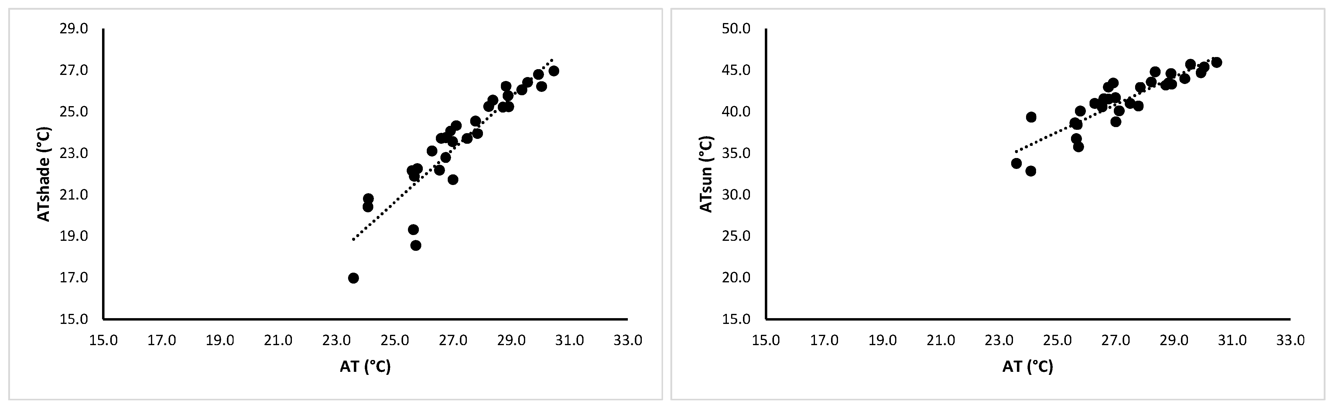
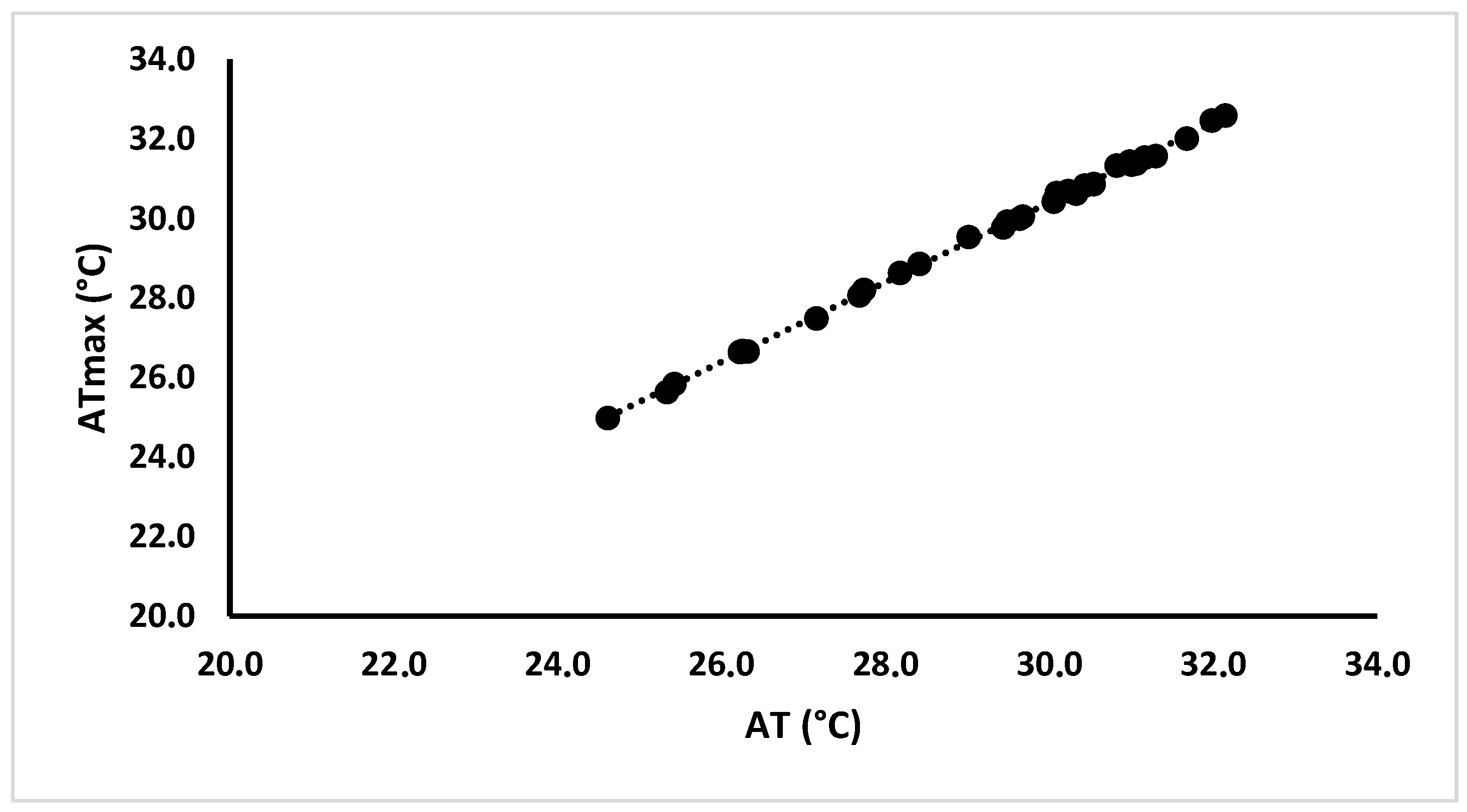
2.2.1. Apparent Temperature Definition

The apparent temperature AT is an index of thermal stress that an individual experiences in terms of average temperature and average relative humidity. Starting from meteorological database, we calculate daily values of apparent temperature (in °C) following the formula

$$\mathrm{A}\mathrm{T}=0.92\mathrm{T}+0.22\mathrm{V}\mathrm{P}-1.3$$

(1)

where T is the daily average temperature in °C (application range: −10 °C~40 °C) and VP is the vapor pressure in hPa defined as $\mathrm{V}\mathrm{P}=0.061 {\mathrm{R}\mathrm{H} 10 }^{7.5\mathrm{T}/(237.3+\mathrm{T})}$, where RH is the average relative humidity in percentage [30,31].

We calculate daily AT from June 1st to September 30th (Summer Days SDs, N = 116 days for 2013, N = 122 for 2014, N = 115 for 2015, and N = 111 for 2016). This index simultaneously accounts for the discomfort caused by both high temperatures and high relative humidity.

In order to test the dependence of AT values also by other meteorological parameters, we evaluate if wind speed and radiance produce variations in the behavior of AT values and if the AT pattern changes introducing the daily maximum values of temperature and relative humidity in the Formula (1). These steps are important because AT values can be affected by orography or local climatic conditions of the examined area that determine specific wind patterns or strong thermic excursion.

To this aim we calculate AT_shade values, introduced in the formula wind speed (WS m/s),

$${\mathrm{A}\mathrm{T}}_{\mathrm{s}\mathrm{h}\mathrm{a}\mathrm{d}\mathrm{e}}=1.04\mathrm{T}+0.2\mathrm{V}\mathrm{P}-0.65\mathrm{W}\mathrm{S}-2.7$$

(2)

AT_sun values are introduced in the formula for both wind speed and radiance (Q in W/m²)

$${\mathrm{A}\mathrm{T}}_{\mathrm{s}\mathrm{u}\mathrm{n}}=1.07\mathrm{T}+0.24\mathrm{V}\mathrm{P}-0.92\mathrm{W}\mathrm{S}+0.044\mathrm{Q}-1.8$$

(3)

and we compare the obtained values. Furthermore, we calculate the apparent temperature using the maximum values of daily temperature and the maximum values of daily relative humidity (AT_max), and we evaluate the difference between AT_max values and AT values calculated using the average values of daily temperature and the average values of daily relative humidity

2.2.2. Hot Days and Apparent Temperature Heat Wave Definition

Based on the AT values, we classify each day in a scale of increasing discomfort, as in Sung et al. 2023 [31]. This classification defines the level of heat stress risk classified from Caution or Hot Day with rank 1 (HD₁) to Extreme danger with possible health-related problems Hot Day with rank 4 (HD₄) (

Table 2. Classification of Hot Days in four classes of risk [30].

AT (°C)	HD Rank	Risk Levels	Classification	Health Problems
28–31	HD1	Slight	Caution	Fatigue possible with prolonged exposure.
32–34	HD2	Moderate	Extreme Caution	Sunstroke, heat cramps and heat exhaustion are likely with continued physical activity.
35–39	HD3	Strong	Danger	Sunstroke, heat cramps and heat exhaustion are possible. Heat stroke is likely with continued physical activity.
≥40	HD4	Extreme	Extreme Danger	Heat stroke is highly likely and imminent.

Legend: AT = apparent temperature; HD = Hot Days.

).

Moreover, in order to quantify the persistence of discomfort conditions, we introduce apparent temperature heat waves (ATHW), taking into account the daily risk classification. We define ATHW as the periods with at least 5 consecutive days defined as Hot Days [25].

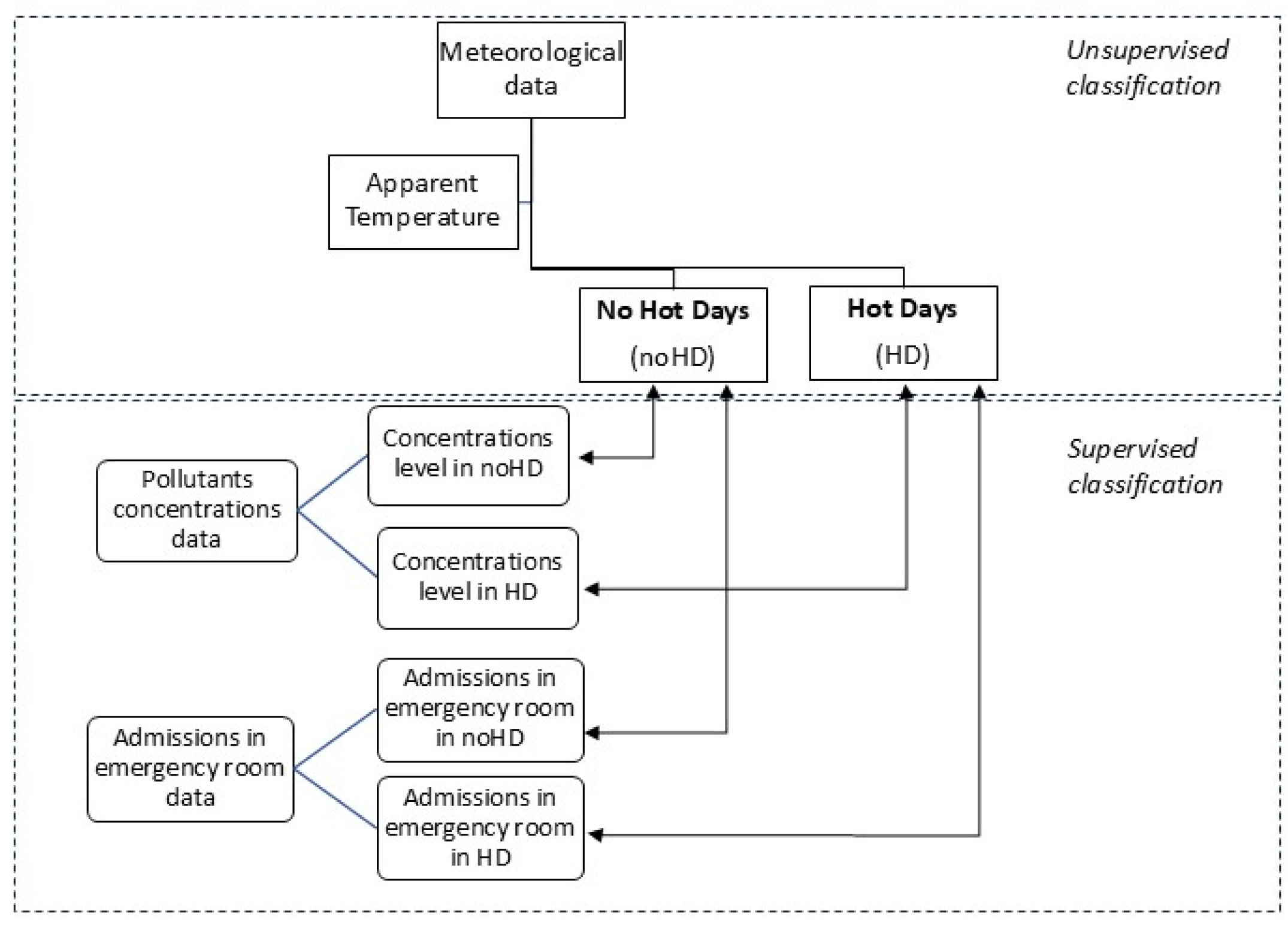
2.2.3. Multidimensional Statistical Data Analysis

In order to establish the possible influence of the environmental conditions of discomfort on admission to the emergency room and the onset of specific pathologies, we apply the classification procedure illustrated in Figure 2. In the first step, we carry out an unsupervised classification of the Summer Days (SD), separating them into Hot Days (HDs) and no Hot Days (noHDs) on the basis of AT values and the levels of risk shown in Table 2. In the second step, for each group of days, we calculate the centroids (mean values with respective standard deviation) of the concentrations of atmospheric pollutants (PM10 and Nox) and the centroid of admission to the emergency room (supervised classification). For testing the differences, we apply a two-tailed paired t-test. If the observed differences are statistically significant, we may affirm that the examined descriptor has a different behavior in the different subgroups of days, and consequently, this variable may be used to describe the effects of the environmental discomfort [25].

3. Results

3.1. Apparent Temperature and HD Identification

In

Table 3. Univariate statistical descriptors of meteorological data.

Year	N	Tm ± ΔTm (°C)	Range T (°C)	RHm ± ΔRHm (%)	Q ± ΔQ (W/m2)	WSm ± ΔWSm (m/s)	Range WSmax (m/s)
2013	116	25 ± 3	17.5–32.0	62 ± 8	264 ± 60	3.2 ± 1.7	4.4–19.6
2014	122	24 ± 2	18.0–29.5	64 ± 9	276 ± 64	3.2 ± 1.6	4.7–31.8
2015	115	26 ± 3	18.6–31.0	62 ± 10	281 ± 65	3.2 ± 1.8	2.5–14.7
2016	121	24 ± 3	19.2–30.4	67 ± 8	270 ± 65	3.4 ± 1.7	3.0–24.9

Legend: N = number of examined days; T_m ± ΔT_m= mean value of daily average temperature and standard deviation; range T = minimum and maximum value of daily average temperature; RH_m ± ΔRH_m = mean value of daily average relative humidity and standard deviation; Q ± ΔQ = mean value of daily radiance and standard deviation; WS_m ± ΔWS_m = mean value of daily average wind speed and standard deviation; range WS_max = minimum and maximum value of daily maximum wind speed.

, we show univariate statistical descriptors of meteorological data collected by the ARPA network during summers from 2013 to 2016. For all the years, we analyzed data collected from June 1st to September 30th.

As a first step, we evaluate if the wind speed and radiance produce variations in the behavior of AT values. This step is important because AT values can be affected by orography or local climatic conditions of the examined area.

In the investigated area, the correlation among AT, AT_shade, and AT_sun is very high. As an example, Figure 3 shows the scatterplots AT vs. AT_shade and AT vs. AT_sun for August 2014. In both cases, the correlation coefficient is higher than 0.85: ρ(AT-AT_shade) = 0.92 and ρ(AT-AT_sun) = 0.89 (d.f = 30 and p = 0.01). For the other examined periods, we find the same results. This indicates that AT, AT_shade, and AT_sun in the examined area are equivalent, and radiance and wind speed do not influence the classification HD/noHD.

As a second step, we calculate the apparent temperature using the maximum values of daily temperature and the maximum values of daily relative humidity (AT_max), and we evaluate the difference between AT_max values and AT values calculated using the average values of daily temperature and the average values of daily relative humidity. In Figure 4, the correlation between AT_max and AT calculated in the period June–September 2015 is shown (ρ = 0.98 with d.f. = 92 and p = 0.01)

Based on this observation, and in accordance with what has been observed for AT_shade and AT_sun, in the following, we use only daily average values of temperature and daily average values of relative humidity to calculate daily apparent temperature values.

Finally, starting from Table 1, we classify the daily apparent temperature of investigated period 2013–2016, and consequently, we individuate the HD and the ATHW. The results are shown in

Table 4. Hot Days and apparent temperature heat waves with respective lengths.

		2013	2014	2015	2016
noHD	No Risk	78 days (67%)	107 days (88%)	63 days (54%)	91 days (75%)
HD1	Slight	38 days (33%)	15 days (12%)	48 days (42%)	30 days (25%)
HD2	Moderate	0	0	4 (4%)	0
HD3	Strong	0	0	0	0
HD4	Extreme	0	0	0	0
ATHW		3	1	3	3
		d1 = 7 days	d1 = 5 days	d1 = 28 days	d1 = 5 days
		d2 = 17 days		d2 = 12 days	d2 = 7 days
		d3 = 5 days		d3 = 5 days	d3 = 12 days

Legend: noHD = no Hot Days; HD = Hot Days; ATHW = Apparent Temperature Heat Waves; SD = Summer Days; d = length of ATHW.

.

3.2. Pollution Level During HD

In

Table 5. PM₁₀ monthly concentrations (all values are expressed in µg/m³).

	Year	June	July	August	September
St1—Caldarola	2013	23	28	27	25
	2014	23	22	21	20
	2015	24	31	24	27
	2016	24	25	21	22
St2—Carbonara	2013	14	11	20	32
	2014	35	31	32	32
	2015	25	30	28	29
	2016	24	25	22	23
St3—CUS	2013	16	19	18	15
	2014	17	17	20	15
	2015	20	27	28	28
	2016	15	19	21	20
St4—Kennedy	2013	20	25	25	19
	2014	24	18	20	20
	2015	22	29	23	25
	2016	21	24	20	20

and

Table 6. NO_x monthly concentrations (all values are expressed in µg/m³).

	Year	June	July	August	September
St1—Caldarola	2013	36	38	33	43
	2014	40	35	33	41
	2015	31	44	42	61
	2016	35	32	29	50
St2—Carbonara	2013	26	24	19	24
	2014	22	16	16	21
	2015	31	32	26	26
	2016	26	25	19	30
St3—CUS	2013	29	28	34	33
	2014	25	19	19	31
	2015	21	34	19	29
	2016	23	24	20	30
St4—Kennedy	2013	17	18	19	25
	2014	24	17	29	24
	2015	31	43	30	33
	2016	26	28	24	35

, we show mean monthly values of PM₁₀ and NO_X concentrations measured in four sampling stations located in Bari from June 1st to September 30th.

To put in evidence the difference in pollutants concentrations among Summer Days, days classified as HD (HD₁ + HD₂), and days classified as noHD, we separately consider the two last groups and calculate their centroids [25]. To test the differences, we apply a two-tailed t-test. The results are shown in

Table 7. Centroids (mean values of daily pollutant concentrations) calculated for Summer Days, Hot Days, and no Hot Days (all values are expressed in µg/m³). The cases in which the differences are statistically significant are in bold.

Year		m (PM10)	sd (PM10)	m (NOX)	sd (NOX)
2013	SD (116 days)	21.8	7.0	27.6	17.9
	HD1 (38 days)	25.3 Δm% = +16% p = 0.01	6.2	30.1	20.8
	noHD (78 days)	20.2	6.8	26.5	16.3
2014	SD (122 days)	20.9	8.9	25.7	14.9
	HD1 (15 days)	28.5 Δm% = +36% p = 0.01	7.8	26.6	16.4
	noHD (107 days)	20.2	8.7	25.6	14.7
2015	SD (115 days)	26.7	12.1	33.0	20.5
	HD1 + HD2 (52 days)	34.3 Δm% = +28% p = 0.01	13.4	37.3 Δm% = +13% p = 0.01	23.8
	noHD (63 days)	21.0 Δm% = −21% p = 0.01	7.4	29.9 Δm% = −9% p = 0.01	17.1
2016	SD (121 days)	21.1	7.0	28.3	19.1
	HD1 (30 days)	24.1 Δm% = +14% p = 0.01	5.0	29.1	17.1
	noHD (91 days)	20.1	7.3	28.0	19.7

Legend: m = mean value; sd = standard deviation; Δm% = percentage difference respect to mean value shown in Table 5 and Table 6; SD = Summer Days HD = Hot Days; noHD = no Hot Days.

.

We also calculate the concentrations of pollutants during the ATHWs for each year in order to better understand their behavior (

Table 8. Mean value of daily pollutant concentrations calculated for ATHW (all values are expressed in µg/m³).

Year			Date	m (PM10)	m (NOX)
2013	SD			21.8	27.6
	d1	7 days	17–23 June	26.3	36.5
	d2	17 days	24 July–9 August	27.1	31.6
	d3	5 days	11–15 August	20.5	21.2
2014	SD			20.9	25.7
	d1	5 days	10–14 August	26.7	28.4
2015	SD			26.7	33.0
	d1	28 days	14 July–10 August	29.4	35.2
	d2	12 days	25 August–5 September	31.3	39.4
	d3	5 days	15–19 September	50.6	47.0
2016	SD			21.1	28.3
	d1	5 days	1–5 July	22.7	31.4
	d2	7 days	8–14 July	27.2	30.0
	d3	12 days	21 July–1 August	23.4	28.3

Legend; SD = summer days, d = length of ATHW, m = mean value.

).

3.3. Access to Emergency Room During HD

To evaluate the influence of thermal discomfort on emergency room access, we examine a database of daily access to the emergency room in the Bari Policlinico “Giovanni XXIII” from 2013 to 2016 for all the 33 codes in Table 1. As a first step, for each year, we calculate the mean value of daily access (MDA expressed in access/day) for different periods: year (MDA_year), Summer Days (MDA_SD), and Hot Days (MDA_HD). Moreover, we calculate the increase percentage of access to the emergency room with respect to the entire year (

Table 9. Mean value of daily access to the emergency room calculated for the year (MDA_y), for the Summer Days (MDA_SD), and for the Hot Days (MDA_HD) with the increase percentage (all values are expressed in access/day).

	2013	2014	2015	2016
MDAy	208	221	206	195
MDASD	230 +11%	233 +5%	215 +4%	199 +2%
MDAHD	242 +16%	240 +9%	225 +9%	197 +1%

Legend: MDA_y = mean value of daily access in the year; MDA_SD = mean value of daily access for the Summer Days; MDA_HD = Mean value of Daily Access for the Hot Days.

).

In order to analyze the impact on specific pathologies and to highlight those influenced in the short term by environmental discomfort, it is necessary to set two thresholds, both on the number of daily accesses for each code and on the observed variations. We chose to consider only cases where MDA > 6 (MDA_y/N_cod) and the percentage variation is above 10% (±2σ).

The results put in evidence that the codes showing variations during SD and HD for all the years are ENT disorders and dermatological symptoms or disorders.

Table 10. Mean value of daily access to the emergency room for specific codes calculated for the year (MDA_y), for the Summer Days (MDA_SD) and for the Hot Days (MDA_HD) with the increase percentage (all values are expressed in access/day).

		MDAy	MDASD	MDAHD
ENT disorders	2013	12	16 (+33%)	21 (+75%)
	2014	13	15 (+15%)	19 (+46%)
	2015	11	15 (+36%)	18 (+64%)
	2016	10	12 (+20%)	13 (+30%)
Dermatological sym/disorders	2013	11	14 (+27%)	16 (+45%)
	2014	11	14 (+27%)	16 (+45%)
	2015	10	13 (+30%)	13 (+30%)
	2016	9	11 (+22%)	11 (+22%)

Legend: MDA_y = mean value of daily access in the year; MDA_SD = mean value of daily access for the Summer Days; MDA_HD = mean value of daily access for the Hot Days.

shows the percentage variation for each examined year.

4. Discussion

In this paper, we study apparent temperature, putting in evidence the days of discomfort and the behavior of air pollutant concentrations and emergency room admissions during these days. All the data were collected in Bari, Southern Italy.

We selected a biometeorological index, apparent temperature, able to put in evidence the days with higher discomfort, as shown in Sung et al. 2023. [31] We verify, as shown in Figure 3, that AT is not influenced by solar irradiance and wind speed in the examined area. So, we calculate AT as in (1). Moreover, we compare AT calculated by means of daily maximum temperature and AT calculated by means of daily average temperature. We do not highlight significant differences, so we use daily average temperature for calculating AT (Figure 4). All these observations are linked to the meteorological and orographic characteristics of the investigated area. We have examined a flat coastal area (Figure 1); therefore, in sites with different characteristics (internal, mountainous, etc.), it will be necessary to repeat the tests to evaluate which is the best way to calculate AT.

Starting from AT values, we define the Hot Days on the basis of the classification in Table 2. As can be observed in Table 4, HDs exceed 25% in the whole period analyzed, except for the summer of 2014 (% HD = 12%). The summer of 2014 is characterized by a lower mean temperature and maximum temperatures below 30 °C. During 2013 and 2016, the number of HDs is high, but they are all first level HDs (slight risk) (Table 2). On the contrary, during 2015, we recorded the highest number of HDs (52 days) and also four second level HDs (moderate risk).

Regarding the persistence of thermal discomfort conditions, for each year, we highlight the consecutive HDs defining the apparent temperature heat waves (ATHWs). The length of these ATHWs is shown in Table 4. The most relevant ATHWs are d₂ = 17 days from July 24th to August 9th followed by d₃ = 5 days from August 11th to 15th in summer 2013; d₁ = 28 days from July 14th to August 10th and d₂ = 12 days from August 25th to September 5th in summer 2015; d₃ = 12 days from July 21st to August 1st in summer 2016.

From the analysis of the pollution data, we obtain that 2015 shows the higher mean values of both PM₁₀ (26.7 ± 12.1 µg/m³) and NO_X (33.0 ± 20.5 µg/m³), as shown in Table 7, but as we said earlier, 2015 was also the hottest examined year. During 2015, we recorded the highest mean values of temperature (26 ± 3 °C) and irradiance (281 ± 65 W/m²), and at same time, we recorded the lowest mean values of wind speed maximum values (14.7 m/s) and relative humidity (62 ± 10%) (Table 3).

It is interesting to analyze the behavior of pollutant concentrations during HDs and ATHWs.

The analysis of the centroids highlights that on HDs, the concentrations of PM₁₀ and NO_X are always higher. For all the examined years, the mean value of PM₁₀ concentration measured during HDs is significantly higher than the mean value measured during noHDs (2013 +16%, 2014 +36%, 2015 +28%, 2016 +14%) (Table 7). Moreover, we would note that in 2014, there were only 15 HDs and they were non-consecutive (there was only one ATHW of 5 days) and yet that the concentrations of PM₁₀ were 36% higher than on other days of the summer. This indicates that the peaks of PM₁₀ concentrations have always occurred on days classified as at risk of thermal discomfort. Instead, in 2015, there are 52 HDs with very long ATHWs; in this case, both the concentrations of PM₁₀ and NO_X are significantly higher than the average (+28% and +13%, respectively), indicating that for the entire period in which the weather conditions were uncomfortable, the air quality was also bad (Table 7).

The results shown in Table 8 better highlight the link between thermal discomfort and pollutant concentrations. Analyzing the pollutant concentrations during ATHWs, we note that persistence of unfavorable weather conditions and a general worsening of air quality are often linked. In 2013, we note that a single day of rain, 10 August 2013, in which we record 0.25 mm, that interrupts an ATHW is enough to reduce the atmospheric concentrations of both NO_X and PM₁₀. While in 2016, two days (6 July 2016, 7 July 2016) of overcast skies without precipitation cause a concentration increase in PM₁₀ and a slight decrease in the concentrations of NO_X due to a little decrease in Q (−23%) These behaviors are like what has been found in other papers [32,33] (

Table 11. Daily pollutants concentrations in specific days (shown in italic) in which an interruption of ATHW was observed (all values are expressed in µg/m³).

Pollutants	Date	St1-Caldarola	St2-Carbonara	St3-CUS	St4-Kennedy
PM10	9 August 2013	39	13	23	36
	10 August 2013	20	8	12	19
	11 August 2013	21	13	12	20
	5 July 2016	22	21	10	21
	6 July 2016	25	29	16	24
	7 July 2016	25	25	25	20
	8 July 2016	31	31	27	24
NOX	9 August 2013	40	17	24	21
	10 August 2013	30	18	13	17
	11 August 2013	18	12	6	11
	5 July 2016	24	28	10	26
	6 July 2016	41	32	25	34
	7 July 2016	33	33	23	12
	8 July 2016	37	37	31	26

).

Analyzing the data of emergency service, as shown in Table 9, during SDs, the mean value of the access to the emergency room is higher than the mean values of the year. Moreover, the amount of daily access increases during HDs. There seems to be a systematic increase in emergency room access on days characterized by high AT and poor air quality. We can also observe a decrease in daily access from 2013 to 2016, which is also reflected in the percentages of increase with respect to the entire year. In 2013, during Hot Days, there was a 27% increase in the amount of mean daily access; in 2016, this percentage decreased to 3%. This behavior may suggest greater awareness of the population for having lifestyles protecting from high temperatures or more generally from bad environmental conditions.

Finally, we highlight pathologies leading to increased access to emergency room during days having bad environmental conditions. If we examine the single access code, we note that the codes that show variability are ENT disorders (from +30% to +75%) and dermatological symptoms or disorders (from +22% to 45%) (Table 10) These results are in agreement with what was found in the bibliography [34,35,36,37].

Starting from our results, we may affirm that the selected biometeorological index, based on daily average values of temperature and relative humidity, is able to put in evidence the days with high discomfort.

The classification in Hot Days and no Hot Days and the persistence of the discomfort conditions defined by means of ATHWs effectively allow us to analyze the consequences of meteorological conditions on human health.

The analysis of the concentrations of PM₁₀ and NO_X compared to our HD classification shows that the air quality worsens on days when the thermal discomfort is higher. Moreover, PM₁₀ and NO_X show different behaviors. PM₁₀ concentrations increase during days of higher thermal discomfort, while NO_X increases less noticeably.

The analysis of access to the emergency room shows that on the days of greatest thermal discomfort, requests for health services increase. This is particularly true for ENTs and dermatological diseases.

5. Conclusions

Ongoing climate change directly affects human health. We focused our attention on how meteoclimatic conditions can affect emergency room admissions in a large coastal city in southern Italy, also taking into account variations in air quality.

In this field it is difficult to find general results because the factors influencing human health (meteorological factors, environmental factors, lifestyles of the population) have local specificities, so it is very important to propose a data analysis procedure that is instead free from specific hypotheses or specific modelling parameters.

The procedure developed in this paper is based only on observational data and is independent from modelling hypothesis; therefore, it can be easily generalized in contexts with different geographic/orographic characteristics or different levels of urbanization/industrialization.

The results of our study show that the analysis of emergency room access can be useful to evaluate the impact on human health of unfavorable climatic and environmental conditions in the summer period.

Furthermore, the results obtained can also be used to optimize resources in the management of the emergency room. Further developments in this work may involve elaborating a new index that accounts for both meteorological parameters and pollutant concentrations to provide synthetic information on environmental discomfort and not just weather-related discomfort.

References

1. Balsari, S.; Dresser, C.; Leaning, J. Climate Change, Migration, and Civil Strife. Curr. Environ. Health Rep. 2020, 7, 404–414. [Google Scholar] [CrossRef]
2. Castro, B.; Sen, R. Everyday Adaptation: Theorizing climate change adaptation in daily life. Glob. Environ. Change 2022, 75, 102555. [Google Scholar] [CrossRef]
3. Xu, R.; Yu, P.; Liu, Y.; Chen, G.; Yang, Z.; Zhang, Y.; Wu, Y.; Beggs, P.; Zhang, Y.; Boocock, J.; et al. Climate change, environmental extremes, and human health in Australia: Challenges, adaptation strategies, and policy gaps. Lancet Reg. Health West Pac. 2023, 40, 100936. [Google Scholar] [CrossRef]
4. Canturk, U.; Kulaç, S. The effects of climate change scenarios on Tilia ssp. in Turkey. Environ. Monit. Assess. 2021, 193, 771. [Google Scholar] [CrossRef] [PubMed]
5. Ventura, F.; Poggi, G.M.; Vignudelli, M.; Bosi, S.; Negri, L.; Fakaros, A.; Dinelli, G. An Assessment of Proso Millet as an Alternative Summer Cereal Crop in the Mediterranean Basin. Agronomy 2022, 12, 609. [Google Scholar] [CrossRef]
6. Krivoguz, D.; Bespalova, E.; Zhilenkov, A.; Degtyarev, A.; Zinchenko, E. Unveiling climate–land use and land cover interactions on the Kerch Peninsula using structural equation modeling. Climate 2024, 12, 120. [Google Scholar] [CrossRef]
7. Wang, H.L.; Wu, K.; Liu, Y.M.; Sheng, B.S.; Lu, X.; He, Y.P.; Xie, J.L.; Wang, H.C.; Fan, S.J. Role of heat wave induced biogenic VOC enhancements in persistent ozone episodes formation in Pearl River Delta. J. Geophys. Res. Atmos. 2021, 126, e2020JD034317. [Google Scholar] [CrossRef]
8. Wang, Z.Q.; Luo, H.L.; Yang, S. Different mechanisms for the extremely hot central-eastern China in July-August 2022 from a Eurasian large-scale circulation perspective. Environ. Res. Lett. 2023, 181, 024023. [Google Scholar] [CrossRef]
9. Gössling, S.; Neger, C.; Steiger, R.; Bell, R. Weather, climate change, and transport: A review. Nat. Hazards 2023, 118, 1341. [Google Scholar] [CrossRef]
10. Kiarsi, M.; Amiresmaili, M.; Mahmoodi, M.R.; Farahmandnia, H.; Nakhaee, N.; Zareiyan, A.; Aghababaeian, H. Heat waves and adaptation: A global systematic review. J. Therm. Biol. 2023, 116, 103588. [Google Scholar] [CrossRef]
11. Yadav, N.; Rajendra, K.; Awasthi, A.; Singh, C. Systematic exploration of heat wave impact on mortality and urban heat island: A review from 2000 to 2022. Urban Clim. 2023, 51, 101622. [Google Scholar] [CrossRef]
12. Perčič, S.; Bitenc, K.; Pohar, M.; Uršič, A.; Cegnar, T.; Hojs, A. Assessing heatwave-related deaths among older adults by diagnosis and urban/rural areas from 1999 to 2020 in Slovenia. Climate 2024, 12, 148. [Google Scholar] [CrossRef]
13. Cicci, K.R.; Maltby, A.; Clemens, K.K.; Vicedo-Cabrera, A.M.; Gunz, A.C.; Lavigne, E.; Wilk, P. High temperatures and cardiovascular related morbidity: A scoping review. Int. J. Environ. Res. Public Health 2022, 19, 11243. [Google Scholar] [CrossRef]
14. Jin, J.; Xu, Z.; Cao, R.; Wang, Y.; Zeng, Q.; Pan, X.; Huang, J.; Li, G. Long-term apparent temperature, extreme temperature exposure, and depressive symptoms: A longitudinal study in China. Int. J. Environ. Res. Public Health 2023, 20, 3229. [Google Scholar] [CrossRef]
15. Horváth, L.; Verzár, Z.; Csákvári, T.; Szapáry, L.; Domján, P.; Bálint, C.; Khatatbeh, H.; Ali, A.M.; Pakai, A. The impact of meteorological factors on stroke incidence in the Transdanubian Region of Hungary. Climate 2024, 12, 160. [Google Scholar] [CrossRef]
16. Ragettli, M.S.; Saucy, A.; Flückiger, B.; Vienneau, D.; de Hoogh, K.; Vicedo-Cabrera, A.M.; Schindler, C.; Röösli, M. Explorative assessment of the temperature–mortality association to support health based heat warning thresholds: A national case-crossover study in Switzerland. Int. J. Environ. Res. Public Health 2023, 20, 4958. [Google Scholar] [CrossRef] [PubMed]
17. Rai, M.; Stafoggia, M.; de’Donato, F.; Scortichini, M.; Zafeiratou, S.; Fernandez, L.V.; Zhang, S.Q.; Katsouyanni, K.; Samoli, E.; Rao, S. Heat related cardiorespiratory mortality: Effect modification by air pollution across 482 cities from 24 countries. Environ. Int. 2023, 174, 107825. [Google Scholar] [CrossRef]
18. Davis, R.E.; Novicoff, W.M. The impact of heat waves on emergency department admissions in Charlottesville, Virginia, U.S.A. Int. J. Environ. Res. Public Health 2018, 15, 1436. [Google Scholar] [CrossRef]
19. Wu, W.J.; Hutton, J.; Zordan, R.; Ranse, J.; Crilly, J.; Tutticci, N.; English, T.; Currie, J. Scoping review of the characteristics and outcomes of adults presenting to the emergency department during heatwaves. Emerg. Med. Australas. 2023, 35, 903. [Google Scholar] [CrossRef]
20. Shin, J.Y.; Kang, M.; Kim, K.R. Outdoor thermal stress changes in South Korea: Increasing interannual variability induced by different trends of heat and cold stresses. Sci. Total Environ. 2022, 805, 150132. [Google Scholar] [CrossRef]
21. Wong, H.T.; Nguyen, T.D. The need for location specific biometeorological indexes in Taiwan. Front. Public Health 2022, 10, 927340. [Google Scholar]
22. Maharana, P.; Kumar, D.; Das, S.; Tiwari, P.R.; Norgate, M.; Raman, V.A.V. Projected changes in heatwaves and its impact on human discomfort over India due to global warming under the CORDEX-CORE framework. Theor. Appl. Climatol. 2024, 155, 2775. [Google Scholar]
23. Papanastasiou, D.K.; Melas, D.; Kambezidis, H.D. Air quality and thermal comfort levels under extreme hot weather. Atmos. Res. 2015, 152, 4. [Google Scholar]
24. Ni, J.; Zhao, Y.; Li, B.; Liu, J.; Zhou, Y.; Zhang, P.; Shao, J.; Chen, Y.; Jin, J.; He, C. Investigation of the impact mechanisms and patterns of meteorological factors on air quality and atmospheric pollutant concentrations during extreme weather events in Zhengzhou city, Henan Province. Atmos. Pollut. Res. 2023, 14, 101932. [Google Scholar]
25. Ragosta, M.; D’Emilio, M.; Casaletto, L.; Telesca, V. A statistical procedure for analyzing the behavior of air pollutants during temperature extreme events: The case study of Emilia Romagna Region (northern Italy). Appl. Sci. 2021, 11, 8266. [Google Scholar] [CrossRef]
26. ARPA Puglia Data. Available online: https://www.arpa.puglia.it/pagina2839_meteo.html (accessed on 1 January 2025).
27. Telesca, V.; Castronuovo, G.; Favia, G.; Marranchelli, C.; Pizzulli, V.A.; Ragosta, M. Effects of Meteo Climatic Factors on Hospital Admissions for Cardiovascular Diseases in the City of Bari, Southern Italy. Healthcare 2023, 11, 690. [Google Scholar] [CrossRef]
28. Elferchichi, A.; Giorgio, G.A.; Lamaddalena, N.; Ragosta, M.; Telesca, V. Variability of temperature and its impact on reference evapotranspiration: The test case of the Apulia Region (Southern Italy). Sustainability 2017, 9, 2337. [Google Scholar] [CrossRef]
29. ARPA Puglia Data. Available online: https://www.arpa.puglia.it/pagina2795_aria.html (accessed on 1 January 2025).
30. Steadman, R.G. A universal scale of Apparent Temperature. J. Clim. Appl. Meteorol. 1984, 23, 1674. [Google Scholar]
31. Sung, H.M.; Lee, J.H.; Kim, J.U.; Shim, S.; Chung, C.Y.; Byun, Y.H. Changes in Thermal Stress in Korea Using Climate Based Indicators: Present. Day and Future Projections from 1 km High Resolution Scenarios. Int. J. Environ. Res. Public Health 2023, 20, 6694. [Google Scholar] [CrossRef]
32. Liu, Z.; Shen, L.; Yan, C.; Du, J.; Li, Y.; Zhao, H. Analysis of the Influence of Precipitation and Wind on PM2.5 and PM10 in the Atmosphere. Adv. Meteorol. 2020, 2020, 5039613. [Google Scholar]
33. Nagy, G.; Kovács, R.; Szőke, S.; Bökfi, K.A.; Gurgenidze, T.; Sahbeni, G. Characteristics of pollutants and their correlation to meteorological conditions in Hungary applying regression analysis. IDŐJÁRÁS Quart. J. Hung. Meteorol. Serv. 2020, 124, 113. [Google Scholar]
34. Nieratschker, M.; Haas, M.; Lucic, M.; Pichler, F.; Brkic, F.F.; Parzefall, T.; Riss, D.; Liu, D.T. Fluctuations in emergency department visits related to acute otitis media are associated with extreme meteorological conditions. Front. Public Health 2023, 11, 1153111. [Google Scholar]
35. Kam, S.; Hwang, B.J.; Parker, E.R. The impact of climate change on atopic dermatitis and mental health comorbidities: A review of the literature and examination of intersectionality. Int. J. Dermatol. 2023, 62, 449. [Google Scholar] [PubMed]
36. Haas, M.; Lucic, M.; Pichler, F.; Lein, A.; Brkic, F.F.; Riss, D.; Liu, D.T. Meteorological extremes and their impact on tinnitus-related emergency room visits: A time-series analysis. Eur. Arch. Oto-Rhino-Laryngol. 2023, 280, 3997. [Google Scholar]
37. Parker, E.R.; Mo, J.; Goodman, R.S. The dermatological manifestations of extreme weather events: A comprehensive review of skin disease and vulnerability. J. Clim. Change Health 2022, 8, 100162. [Google Scholar]
Figure 1. Study area: on the left, digital elevation model covering the city of Bari and neighboring municipalities (black lines highlight municipal boundaries); on the right, the Corine Land Cover (CLC) 2018, aggregated at the first level. The monitoring station of meteorological parameters, monitoring stations of air quality, and emergency room of Policlinico Giovanni XXIII are shown.
Climate 13 00067 g001
Figure 2. Flow chart of classification procedure.
Climate 13 00067 g002
Figure 3. Scatterplots AT vs. ATshade (R2 = 0.84) and AT vs. ATsun (R2 = 0.79)for August 2014.
Climate 13 00067 g003
Figure 4. Scatterplots ATmax vs. AT (R2 = 0.99) for the period June–September 2015.
Climate 13 00067 g004