Article

Rainfall Patterns and Trends on São Miguel Island (Azores, Portugal): A Hierarchical Clustering and Trend Analysis Approach

by
Rui Fagundes Silva
1,2,*,
Rui Marques
1,2,
José Luís Zêzere
3,4 and
Marcelo Fragoso
3,4
1
Research Institute for Volcanology and Risk Assessment, University of the Azores, Rua Mãe de Deus, 9500-321 Ponta Delgada, Portugal
2
Centre for Information and Seismovolcanic Surveillance of the Azores, University of the Azores, Rua Mãe de Deus, 9500-321 Ponta Delgada, Portugal
3
Centre of Geographical Studies, IGOT, University of Lisbon, Rua Branca Edmée Marques, 1600-276 Lisboa, Portugal
4
Associate Laboratory TERRA, Instituto Superior de Agronomia, University of Lisbon, Tapada da Ajuda, 1349-017 Lisboa, Portugal
*
Author to whom correspondence should be addressed.
Climate 2025, 13(11), 238; https://doi.org/10.3390/cli13110238
Submission received: 20 October 2025 / Revised: 15 November 2025 / Accepted: 18 November 2025 / Published: 20 November 2025
(This article belongs to the Section Climate and Environment)

Abstract

This study addressed rainfall patterns and trends on São Miguel Island (Azores, Portugal). Homogeneous rainfall areas were identified using Ward’s hierarchical clustering method. The analysis was performed using monthly rainfall data from 21 rainfall stations, considering the climatological periods of 1978/79–2019/20 (full dataset), 1978/79–2009/10 (oldest sub-dataset), and 2010/11–2019/20 (latest sub-dataset). Four rainfall clusters were identified, with Mean Annual Rainfall (MAP) ranging from 835.8 mm in low-altitude areas to 2925.5 mm in regions with higher elevation. These clusters showed consistent patterns for the analysed periods, although some changes in their composition were observed when considering the oldest and latest sub-datasets. The correlation between altitude and rainfall was strong (R2 up to 0.83), indicating an increase of approximately 196 mm of MAP per 100 m elevation gain. Moreover, no notable variation was observed between the island’s windward and leeward slopes. Rainfall trend analysis using Mann–Kendall and Sen’s slope tests revealed significant declines in both annual and seasonal rainfall in recent years. The strongest decreases occurred in autumn and winter, with trends as steep as −31.6 mm/year and −12.1 mm/year in autumn (both at the Fogo III station). Between the oldest and most recent periods, rainfall reductions reached up to 41% in autumn (P10) and 55% in winter (P10), particularly affecting clusters at lower and mid-altitudes. Although certain stations showed significant declines, the overall trend hints at a potential deviation from projections of global climate change models, as well as from trends identified in previous long-term rainfall studies. The predominantly positive phase of the North Atlantic Oscillation (NAO) observed in recent years has likely contributed, at least partially, to the decrease in the rainfall trend. Overall, the results provide a refined spatial and temporal characterisation of rainfall across São Miguel Island, improving the understanding of local climatic variability and offering valuable insights for regional water management and climate adaptation strategies.

1. Introduction

Rainfall is considered the most important meteorological variable for studying regional climate [1,2]. Planning activities across various societal sectors, including agriculture, energy, water resources, and the hydrological cycle, requires a thorough understanding of the behaviour of this variable. Consequently, knowledge about spatial rainfall patterns is essential for the sustainable management of water resources and for detecting climate variability.
The spatial and temporal variability of rainfall represents one of the main challenges in climatological and hydrological analyses. Its understanding is hindered by the combined influence of multiple factors, which extend beyond local physiographic elements to include processes associated with atmospheric circulation and ocean–atmosphere interactions [3]. In this context, the regionalisation of rainfall emerges as a fundamental tool, enabling the identification of homogeneous patterns and the reduction in the inherent complexity of climate data. A homogeneous rainfall region is an area with statistically similar long-term rainfall patterns [4]. Various approaches have been employed in the scientific literature to examine spatial rainfall patterns, including L-moments [5,6], k-means clustering [7], regional frequency analysis [8], harmonic analysis [9], spatial correlation functions [10], multivariate regression [11], empirical orthogonal functions [12], Pearson’s correlation [13], support vector machines [14], and spatial interpolation [15].
Cluster analysis has been widely applied in the literature for classification tasks [16]. Unlike many statistical methods that depend on predefined theoretical distributions, it groups the data based on observed similarities. Hierarchical and non-hierarchical clustering methods are used, with non-hierarchical methods being more prevalent. Hierarchical clustering arranges clusters hierarchically to reflect similarities or dissimilarities using either a top-down or bottom-up approach. Clusters are formed by repeatedly merging the closest objects based on the shortest distance, until all objects are joined. Ward’s hierarchical method [17] has frequently been used to categorise climatic and hydrologic data, consistently providing more accurate classification results than other methods (e.g., [18,19,20,21,22]). Several studies have employed this method to identify clusters based on climatic variables.
Trends in time series have been identified using various statistical techniques, which are categorised into parametric and non-parametric tests [23,24,25]. Unlike parametric tests, which assume that the data are normally distributed, non-parametric tests make no such assumption [26]. Researchers in climatology, hydrology, and environmental sciences widely favour the non-parametric Mann–Kendall test [27,28] for trend analysis. This test is often paired with Sen’s slope estimator [29,30], another non-parametric method, to quantify the trend magnitude. Together, these methods offer valuable insights into the rate of change within a data series, enhancing the understanding of temporal dynamics.
Rainfall patterns in regions that are influenced by subtropical anticyclones exhibit complex relationships with altitude. Generally, rainfall increases with altitude because of orographic effects. However, this relationship is not always linear and can vary significantly among regions [31]. Windward slopes typically receive more rainfall than leeward slopes because of the orographic effect: as moist air rises, it cools and condenses, forming clouds and rain on the wind-facing slopes, which leads to persistent rainfall patterns [32]. In contrast, leeward slopes tend to be drier, as the descending air warms and dries [33].
The study of rainfall regimes in subtropical anticyclonic regions is fundamental to understanding climate dynamics, improving weather forecasting, and managing water resources. The Azores high-pressure system plays a significant role in modulating rainfall in various regions, including tropical Northeast Africa, Europe, and the Middle East [34,35]. Moreover, research on rainfall regimes in subtropical anticyclonic regions, such as the Azores, is crucial for understanding the impacts of climate change on rainfall patterns and aiding in the development of adaptation and mitigation strategies [36].
The characterisation of rainfall in the Azores remains relatively underexplored. Santos et al. [37] assessed the potential impacts of climate change on the Azores and Madeira islands, focusing on variations in temperature and rainfall. De Lima et al. [38] examined changes in rainfall patterns across Portugal, including the Azores, using long-term annual and monthly rainfall series. Based on long-term monthly rainfall series, Cropper and Hanna [39] identified temporal trends and assessed inter-island variability, as well as the influence of large-scale atmospheric patterns across the Macaronesian archipelagos. Similarly, Hernández et al. [40] analysed daily rainfall in Ponta Delgada (São Miguel Island) over the period of 1873–2012, examining its relationship with large-scale modes of climate variability. Across all studies, the North Atlantic Oscillation (NAO) emerges as the dominant large-scale driver of interannual rainfall variability in the Azores, consistently showing a negative correlation [39,40,41].
Building on these considerations, the main objective of this study was to analyse the spatial and temporal rainfall patterns on São Miguel Island (Azores, Portugal) using a combination of hierarchical clustering and trend analysis methods. To achieve this, the study focused on the following specific objectives: (i) identify homogeneous rainfall areas on the island using Ward’s hierarchical clustering method; (ii) analyse rainfall trends and assess their significance using the Mann–Kendall test together with Sen’s slope estimator; (iii) investigate the influence of the NAO on the temporal variability of rainfall by analysing the longest rainfall series available on the island; and (iv) study the rainfall distribution on the island in relation to the altitude under the broader influence of a subtropical anticyclone.

2. Study Area and Climate Framework

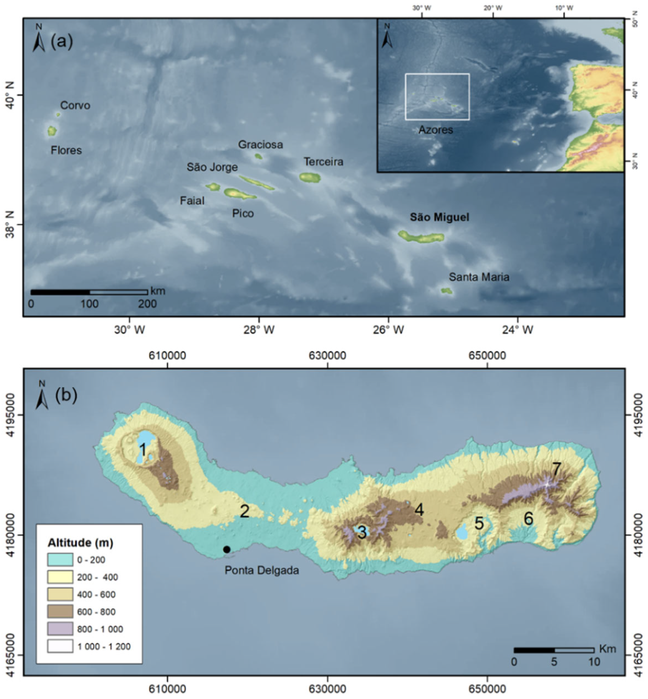
The Azores archipelago, composed of nine volcanic islands in the North Atlantic Ocean (Figure 1a), includes São Miguel, the largest (744.6 km2; 64 km long, 8–15 km wide). The island comprises seven morphological units with distinct geology and geomorphology (Figure 1b), including three active central volcanoes, Sete Cidades [42,43], Fogo [44,45], and Furnas [46,47] and two fissural volcanic systems, Picos [48,49] and Congro [46,50]. Elevation reaches 873 m at Sete Cidades, 949 m at Fogo, and 700 m at Furnas. The Picos Fissural Volcanic System forms gentle slopes below 300 m, while the Congro Fissural Volcanic System rises above 500 m. In the east, the extinct Povoação Volcano and Nordeste Complex [51] form the island’s oldest structures, with the highest elevation (1104 m) located there.
The archipelago is located in a zone of confrontation between tropical and polar air masses in the centre of the North Atlantic basin. Atmospheric circulation and the rainfall regime in the Azores region are primarily influenced by the variability of two main pressure systems: the Icelandic Low and the Azores Subtropical High [52]. During the cold season, the Icelandic Low intensifies, enhancing the activity of disturbances along the polar front and resulting in frequent rainy weather. In summer, the Azores High shifts northward, promoting more stable atmospheric conditions and a marked decrease in rainfall levels. The alternating dominance of these two pressure systems is illustrated in Figure 2, which displays the mean sea-level pressure fields (1991–2020) over the North Atlantic for January and July, highlighting the essential features of the seasonal climatic rhythm of the archipelago (see also Figure 3). This pressure dipole defines the North Atlantic Oscillation (NAO) [53].
According to the Köppen classification, the Azores have a temperate (C-type) climate [52,54], mainly Cfb, with some Csb areas along the coast [55]. The monthly temperature range is low, with values ranging from 14.4 °C in February to 22.6 °C in August, resulting in an amplitude of around 8 °C (Figure 3). Rainfall is evenly distributed throughout the year, with a noticeable decrease in the summer months [52]. The monthly rainfall distribution shows a clear seasonal pattern, with the “rainiest season” spanning from October to March (Figure 3). In contrast, the summer months represent the “driest season”, with the lowest rainfall levels typically occurring in July.
In Ponta Delgada, on average, rainfall occurs on approximately 122 days per year, consisting of 60 rain spells with an average duration of about 2 days. Each rain spell produces an average of 16 mm, with a mean rate of 7.9 mm/day. Around 42% of the annual total rainfall is due to rain spells lasting longer than 3 days [41].
Based on the application of a climate simulation model for island environments [56], São Miguel Island experiences a Mean Annual Rainfall (MAP) ranging from 1200 to 2000 mm near the coast, while in the interior high areas, it can reach as much as 4800 mm [57]. This gradient reflects the influence of prevailing westerly and northwesterly winds, shaped by the mid-latitude westerlies and the Azores High [52]. West- and northwest-facing slopes act as windward areas exposed to moist Atlantic air masses, while eastern and southeastern slopes lie in the leeward zone. Storms are most frequent in winter, though late-summer and autumn cyclones can also cause severe floods and landslides [51].
Climatic diversity across the Azores results from the island’s geomorphological and geological complexity. Several factors—such as central volcanoes; dismantled calderas; lakes; geological formations’ alignment, including monogenetic cones along fracture zones; valleys, which are often associated with fault zones; ventilation corridors; vegetation; and the altitude and orientation of slopes and sea cliffs—significantly contribute to local-scale climate differentiation on each island [58,59,60,61].

3. Materials and Methods

3.1. Rainfall Data Processing

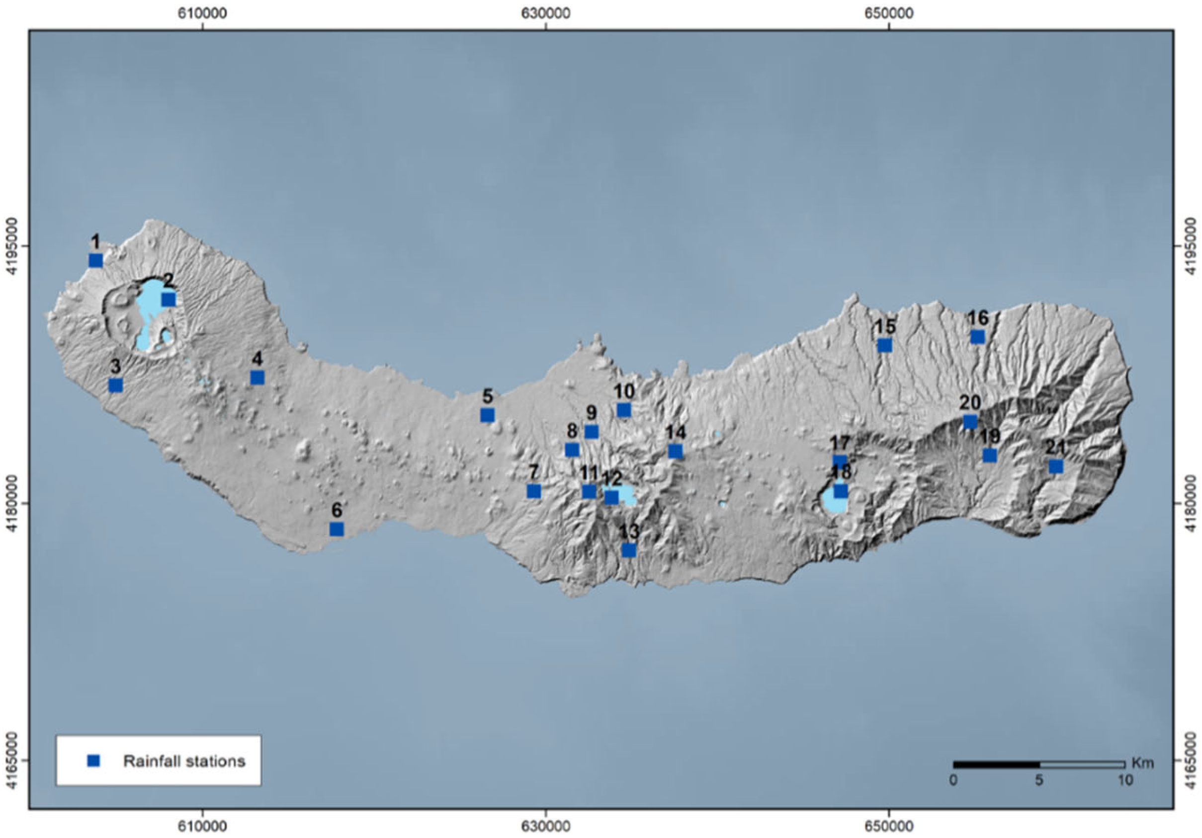
The rainfall data used in this study were collected from 21 rainfall stations. The stations were selected based on the following criteria: (1) data availability from the owning entities and (2) the longest common data period (which corresponds to the climatological years between 1978/79 and 2019/2020). Out of 21 rainfall stations, 17 had data for the period between 1978/79 and 2019/2020, while the remaining 4 had data between 2010/11 and 2019/2020. Table 1 lists the rainfall stations, along with their respective altitudes, periods of record, and key descriptive statistics for the annual time series. The locations of these stations are illustrated in Figure 4.
Monthly rainfall data from each rainfall station were used in this study. The monthly data were aggregated into four three-month periods corresponding to the seasons: autumn (September, October, and November), winter (December, January, and February), spring (March, April, and May), and summer (June, July, and August). From these seasonal datasets, the 10th, 50th, and 90th percentiles were calculated. Additionally, annual rainfall totals and Mean Annual Rainfall (MAP) were computed for each rainfall station. Data quality was assessed through inspection for gaps or anomalies, with no inconsistencies detected. Normality was evaluated using the Shapiro–Wilk [62] and Kolmogorov–Smirnov [63] tests, and homogeneity was verified through the Standard Normal Homogeneity Test (SNHT) [64], Buishand range test [65], Pettitt test [66], and Von Neumann ratio test [67]. Following Wijngaard et al. [68], the series were classified as “useful”, “doubtful”, or “suspect” based on the number of tests rejecting the null hypothesis at the 1% significance level, thereby assessing their suitability for trend and variability analyses.

3.2. Methods

This study was based on the analysis of three distinct temporal periods, determined by the available rainfall station coverage: (1) climatological years from 1978/79 to 2019/2020 (full dataset); (2) climatological years from 1978/79 to 2009/2010 (oldest sub-dataset); and (3) climatological years from 2010/11 to 2019/2020 (latest sub-dataset).
To classify the stations into homogeneous rainfall regions, hierarchical cluster analysis was performed using Ward’s method [17]. This method minimises the total within-cluster variance, ensuring that elements that are grouped together show greater internal similarity than they do with other clusters. The squared Euclidean distance was used as a dissimilarity metric [69]. The number of clusters was validated using the Silhouette Coefficient, which quantifies how well each station fits within its assigned cluster [70].
Hierarchical clustering was performed in three steps to reflect the three temporal datasets: (i) clustering of 17 stations for the full period (1978/79–2019/2020); (ii) clustering of the same 17 stations for the oldest period (1978/79–2009/2010); and (iii) clustering of all 21 stations, including the more recent additions, for the period of 2010/11–2019/2020.
The hierarchical clustering of rainfall stations on São Miguel Island considered 13 variables: Mean Annual Rainfall (MAP) and the 10th, 50th, and 90th percentiles for each season. These percentiles were used in rainfall analysis to better understand the data distribution [71,72]. The 10th percentile (P10) represents frequently occurring low rainfall, helping identify dry periods. The 50th percentile (P50) corresponds to the median rainfall, providing a robust central measure that is unaffected by extreme values. The 90th percentile (P90) highlights high-rainfall events, which are crucial for assessing heavy rainfall conditions and extreme rainfall events. The data were normalised using the Z-score method, standardising the variables to have a mean of zero and a standard deviation of one, thus preventing differences in scale from influencing the clustering results. The Statistical Package for the Social Sciences (IBM SPSS Statistics 30) software was used to derive hierarchical cluster groupings based on these variables.
The variation in the values of variables for each rainfall station within each cluster, as well as the variation between clusters for each of the three periods analysed, was calculated based on the average of each variable and the coefficient of variation (CV).
Rainfall trends were evaluated using the Mann–Kendall (M-K) test [27,28] to assess trend significance and Sen’s slope estimator [29,30] to determine the magnitude of trends. These non-parametric methods are widely recommended for environmental and hydrological time series, as they are robust to missing values and do not require a normal data distribution [73,74]. The analysis of annual and seasonal rainfall trends was conducted using data from the 17 rainfall stations with the longest records, covering the climatological years of 1978/79–2019/20. Stations with data only for more recent periods were excluded, as their rainfall trend analysis would not be statistically representative. Annual rainfall trends were evaluated by analysing the total rainfall recorded for each climatological year at each station. Likewise, seasonal trends were assessed based on the accumulated rainfall for each season.
The correlation between the NAO and the annual and seasonal rainfall series for the same climatological period (1978/79–2019/20) was performed by calculating Spearman’s correlation coefficients. Spearman’s rank correlation and associated p-values capture monotonic relationships and are robust to non-normality and outliers, which are common in rainfall and climate index data [75]. Statistical significance was determined at p < 0.05. The teleconnection index used was the Hurrel NAO index (PC-based), available at https://climatedataguide.ucar.edu/climate-data/hurrell-north-atlantic-oscillation-nao-index-pc-based (accessed on 12 November 2025) [53].
Although the relationship between altitude and rainfall is well known worldwide, the influence of altitude on the identified homogeneous rainfall station groups was also studied. To this end, linear regression graphs were constructed to examine the relationship between altitude and rainfall variables (MAP and the 10th, 50th, and 90th percentiles) across the three considered temporal periods. In addition, Pearson correlation coefficients (r) and their corresponding significance levels (p-values) were calculated to assess the strength and reliability of these relationships.

4. Results

4.1. Analysis of Normalisation and Homogeneity Tests

The results of the Shapiro–Wilk and Kolmogorov–Smirnov normality tests, as well as the classification based on homogeneity tests applied to the annual rainfall time series, are summarised in Table 2. These statistics indicate that the null hypothesis of normality can be rejected for the Fogo III and Espigão da Ponte datasets. Although normality is a prerequisite for some of the subsequent homogeneity tests, all datasets were analysed. It should be noted that the results of the normality and homogeneity tests may affect the validity of the conclusions drawn from the subsequent trend tests and should be interpreted with caution.
While the majority of the datasets are classified as “useful”, some series may not be homogeneous over the entire recorded period. Specifically, the time series for Fogo III, Monte Simplício, and Espigão da Ponte were classified as “doubtful”. This could not be explained based on the available metadata. Moreover, the presence of a significant trend, such as a decreasing trend in a time series, can influence the results of homogeneity tests, potentially leading to their rejection, even in the absence of structural changes in the data [76]. Consequently, for the Fogo III, Monte Simplício, and Espigão da Ponte time series, the results of the trend analysis over the full period should be interpreted with particular caution.

4.2. Clustering of Rainfall Stations and Statistical Analysis

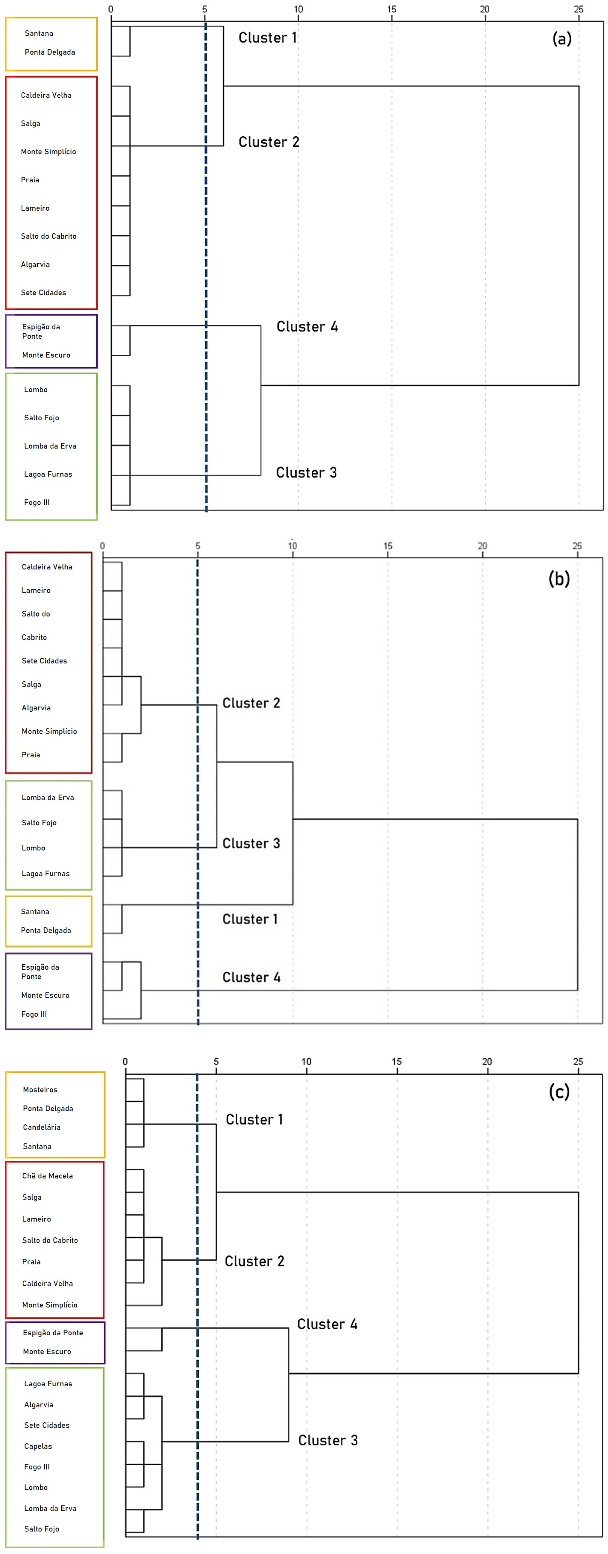
Hierarchical clustering analysis based on Ward’s method identified four main groups of rainfall stations with similar rainfall characteristics (Figure 5). The clustering structure was validated using the Silhouette Coefficient, calculated for k = 2 to k = 8, confirming that four clusters provide the most appropriate classification (Figure 6). The average silhouette values were consistently higher for k = 4 across the full dataset (0.55), the oldest sub-dataset (0.55), and the latest sub-dataset (0.48), indicating a good balance between cluster compactness and separation.
For the full dataset (Figure 5a), Cluster 1 comprises the stations of Santana and Ponta Delgada. Cluster 2 includes eight stations: Caldeira Velha, Salga, Monte Simplício, Praia, Lameiro, Salto do Cabrito, Algarvia, and Sete Cidades. Cluster 3 consists of five stations: Lombo, Salto do Fojo, Lomba da Erva, Lagoa das Furnas, and Fogo III. Lastly, Cluster 4 includes the stations of Monte Escuro and Espigão da Ponte.
In the oldest sub-dataset (Figure 5b), Clusters 1 and 2 remained unchanged, indicating temporal stability in the rainfall patterns of these stations. However, Clusters 3 and 4 underwent reconfiguration. Cluster 3 includes four stations (Lomba da Erva, Salto do Fojo, Lombo, and Lagoa das Furnas), while Cluster 4 includes three stations (Espigão da Ponte, Monte Escuro, and Fogo III). This shift reflects subtle changes in rainfall behaviour, particularly the migration of Fogo III from Cluster 3 to Cluster 4.
The latest sub-dataset (Figure 5c) exhibits a more pronounced reorganisation of the clusters. Cluster 1 expands to include four stations: Mosteiros, Ponta Delgada, Candelária, and Santana. Cluster 2 includes seven stations: Chã da Macela, Salga, Lameiro, Salto do Cabrito, Praia, Caldeira Velha, and Monte Simplício. Cluster 3 consists of eight stations: Lagoa das Furnas, Algarvia, Sete Cidades, Capelas, Fogo III, Lombo, Lomba da Erva, and Salto do Fojo. Cluster 4 maintains the same composition as in the full dataset, with the stations of Espigão da Ponte and Monte Escuro.
Out of the 21 stations analysed, 15 remained in the same cluster throughout the periods considered. Overall, Clusters 1 and 4 show a high degree of temporal stability, reflecting persistent rainfall regimes. In contrast, Clusters 2 and 3 exhibit greater variability, with changes in the number and composition of stations over time. Notably, after 2010, Algarvia and Sete Cidades migrated from Cluster 2 to Cluster 3, suggesting increased rainfall in these areas. The transitional behaviour of the Fogo III station, which shifted between Clusters 3 and 4, highlights the sensitivity of stations that are located in more exposed areas to slight variations in atmospheric circulation patterns.
The mean values of the variables used in the analysis (MAP, P10, P50, and P90) for each cluster are summarised in Table 3. The results highlight the variability in rainfall amounts across different clusters during each considered period. Significant variability in MAP is observed across the clusters. For the full dataset, Cluster 1 exhibits an average MAP of 1059.8 mm, whereas Cluster 4 shows a significantly higher average of 2925.5 mm. Clusters 2 and 3 record average MAP values of 1704.8 mm and 2229.6 mm, respectively. For the oldest sub-dataset, the pattern remains consistent: Cluster 1 maintains a lower average MAP of 1124.2 mm, while Cluster 2 is at 1800.9 mm, Cluster 3 at 2301.0 mm, and Cluster 4 at 2954.4 mm The latest sub-dataset reveals a reduction in overall MAP values and a decrease in the contrast between Clusters 1 and 2, with average MAP vales of 835.8 mm and 1292.6 mm, respectively. Meanwhile, Clusters 3 and 4 also show lower averages compared with previous periods, at 1762.0 mm and 2335.3 mm, respectively. This reduction may indicate a recent shift in rainfall distribution patterns, with a tendency towards drier conditions, especially in the lower-altitude clusters.
The analysis of P10, P50, and P90 values reveals the seasonal fluctuation of rainfall, with higher values typically being recorded in winter, progressively decreasing through spring, and reaching their lowest level in summer. This seasonal trend corroborates the expected annual rainfall cycle. The P10 values are relatively uniform across all seasons and clusters, suggesting a uniformity in the lower limits of rainfall distribution. In contrast, P50 values, representing the median rainfall, show similar trends between clusters in winter and autumn; however, these values diverge significantly in summer, indicating more pronounced differences in median rainfall amounts within each cluster during the drier season. The P90 values, reflecting the upper limits of the rainfall distribution, exhibit significant variability between clusters, particularly in winter and autumn, highlighting the differences in extreme rainfall events across the clusters. During summer, however, differences in P90 values between clusters become less significant, which is consistent with the lower occurrence of extreme rainfall in the drier season.
The coefficient of variation (CV) values of the variables used in the analysis (MAP, P10, P50, and P90) within each cluster are summarised in Table 4, providing insights into intra-cluster homogeneity. For the full dataset, the rainfall stations in each cluster show high similarity, with CV values generally being less than 15%. Clusters 1 and 3 present lower CV values, indicating greater similarity between the stations within these clusters. In Cluster 2, the P10 variable shows higher CV values in autumn, winter, and summer (18.5%, 18.0%, and 19.3%, respectively). In Cluster 4, the greatest heterogeneity within the cluster is observed in the P10 variable for winter and summer (20.9% and 17.3%, respectively).
For the oldest sub-dataset, the CV values remain generally low across clusters, indicating homogeneity among the rainfall stations that make up each cluster. Notably, in Cluster 1, the P90 in summer shows the highest CV value (17.5%), while in Cluster 2, the P10 in spring is the most different among the rainfall stations in the cluster (20.4%). In Cluster 3, the CV values are lower for all variables, reinforcing its homogeneity. Cluster 4 presents its highest CV values in P10 during spring and summer (15.4% and 18.3%, respectively).
In contrast, the latest sub-dataset shows generally higher CV values, frequently exceeding 15%, which reflects increased heterogeneity within clusters. In Cluster 1, the highest value is observed in the P90 variable for summer (27.3%). Cluster 2 exhibits the most variability in P10 during spring (35.8%). Cluster 3 shows the highest CV in P10 during winter (36.3%), and Cluster 4 exhibits the greatest variation in P50 during winter (37.0%). This rise in CV values corresponds to the inclusion of new rainfall stations into the clusters, whose differing characteristics contribute to increased heterogeneity within each group.

4.3. Spatial Distribution of Rainfall Station Clusters

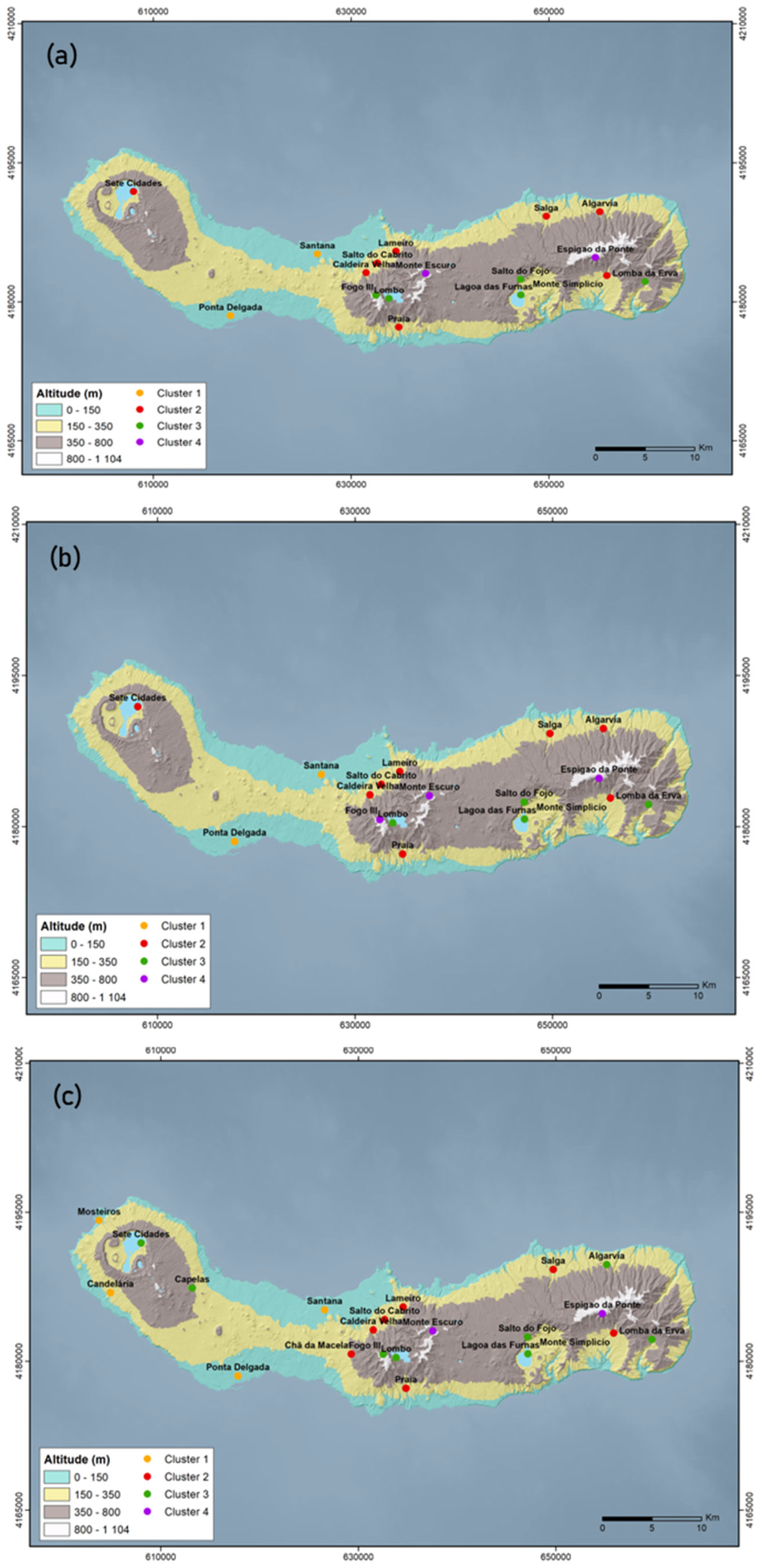
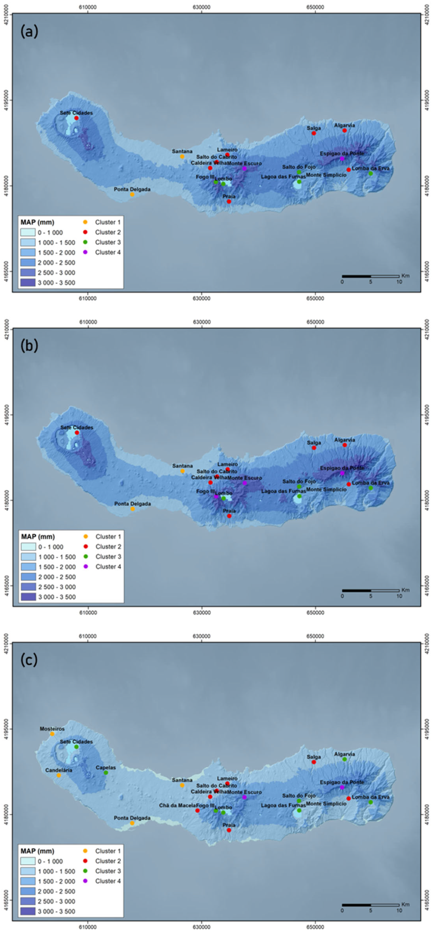
The spatial distribution of the rainfall station clusters provides valuable insights into the relationship between altitude and rainfall patterns across São Miguel Island. Figure 7 illustrates the spatial distribution of stations within each cluster for the full dataset, the oldest sub-dataset, and the latest sub-dataset, respectively, over the hypsometric map of São Miguel Island.
The analysis of the full dataset (Figure 7a) indicates that the geographical positioning of stations within Cluster 1 is confined to lower altitudinal zones, specifically below 150 m. Stations belonging to Cluster 2 are located at intermediate altitudes, ranging from 150 to 350 m. Stations within Cluster 3 are found at higher altitudes, between 350 and 800 m, with the notable exceptions of Lagoa das Furnas station, located inside the Furnas Volcano caldera, and Fogo III station, situated near the rim of the Fogo Volcano caldera. Despite their altitudes of 280 and 893 m, respectively, they are included in Cluster 3. Stations grouped into Cluster 4 are found at the highest altitudes on the island, exceeding 800 m. These results suggest that factors beyond altitude are influencing rainfall patterns.
For both the oldest and latest sub-datasets (Figure 7b,c), Cluster 1 consistently comprises stations located at the lowest altitudes, specifically between 0 and 150 m. Notably, the Candelária station, which is slightly higher at 201 m, is also included in this cluster in the latest sub-dataset (Figure 7c). Rainfall stations belonging to Cluster 2 are located within the intermediate altitude range of 150 to 350 m, whereas rainfall stations in Cluster 3 are generally found at higher altitudes, between 350 and 800 m, except Lagoa das Furnas station. Despite its altitude of 280 m, it consistently remains within Cluster 3, as observed for the full dataset. The analysis of the latest sub-dataset shows that the Sete Cidades and Algarvia stations, located at altitudes of 260 m and 340 m, respectively, are included in Cluster 3 (Figure 7c), despite their altitudes aligning more closely with Cluster 2, underscoring the complex relationship between altitude, geographical factors, and rainfall distribution. Stations belonging to Cluster 4 are located at the highest altitudes on the island (above 800 m), with the latest sub-dataset including Fogo III station in Cluster 3, despite its altitude of 893 m (Figure 7c). This classification emphasises the complex interplay of topography and climate affecting rainfall distribution, suggesting that altitude is a significant, but not exclusive, determinant of rainfall distribution across São Miguel Island.

4.4. Rainfall Trends

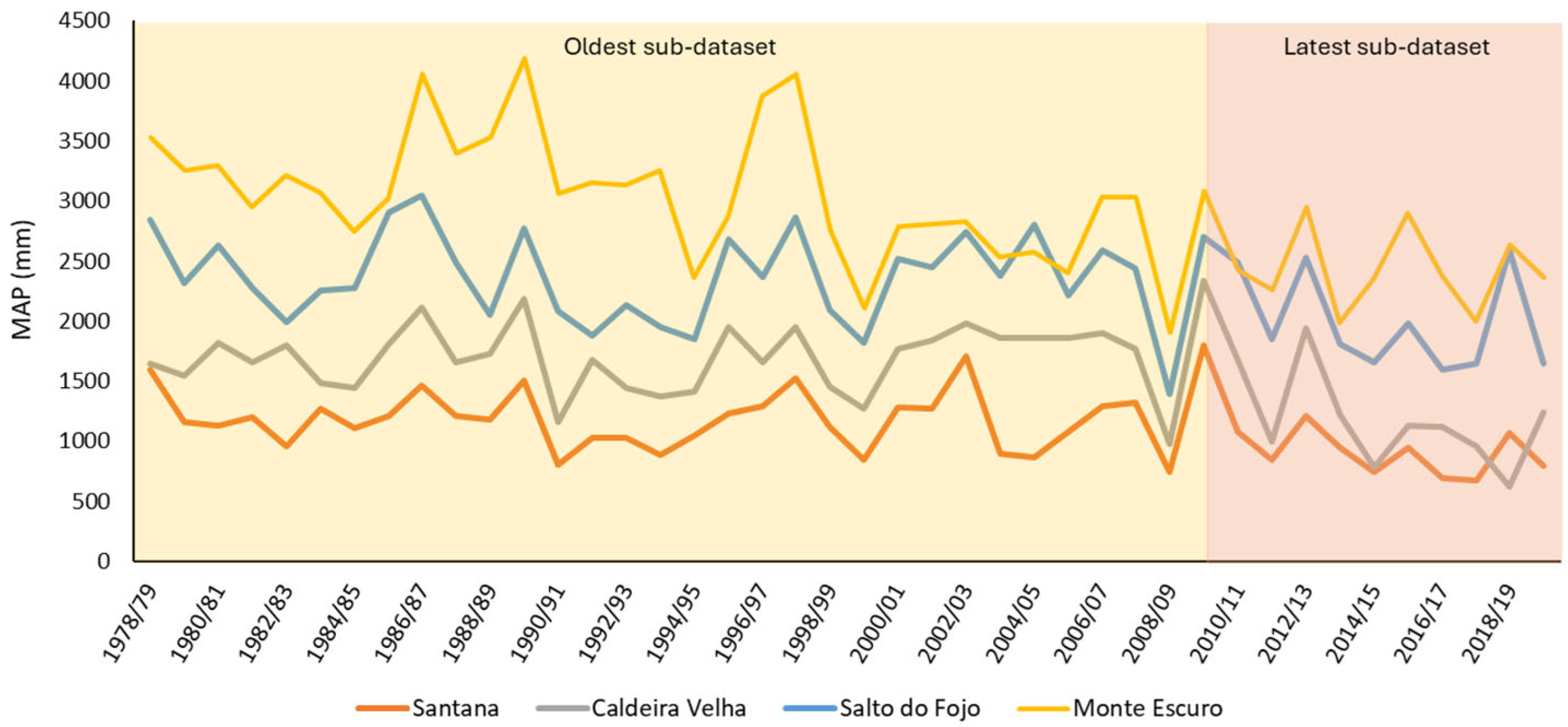
Figure 8 shows the evolution of the Mean Annual Rainfall (MAP) at four representative stations with the most pronounced decreasing rainfall trends—Santana (Cluster 1), Caldeira Velha (Cluster 2), Salto do Fojo (Cluster 3), and Monte Escuro (Cluster 4)—over the climatological years of 1978/79 and 2019/20. During the period corresponding to the oldest sub-dataset (1978/79 to 2009/10), all stations exhibit high interannual variability, reflecting the markedly unstable nature of the regional rainfall regime. However, in the most recent sub-dataset (2010/11 to 2019/20), a general reduction in MAP becomes evident.
Monte Escuro registers the highest annual totals yet shows a declining trend in the most recent decade, particularly with a reduced frequency of years with rainfall exceeding 3000 mm. At Salto do Fojo, the downward trend is more gradual but still evident, with several consecutive years over the last decade in which the rainfall is below the long-term average. At Caldeira Velha, a downward trend in rainfall has also been observed since 2009/10, with several consecutive years recording less than 1200 mm. Santana, while generally exhibiting a more stable pattern, also reveals subtle signs of decreasing rainfall, with an increasing number of recent years registering totals below 1000 mm.
The rate of change in the rainfall variable values between the oldest and latest sub-datasets is summarised in Table 5, which reveals a pronounced decrease in rainfall values, ranging from 20% to 30%. Nonetheless, differences are observed across variables and clusters. The MAP value exhibits a reduction of approximately 25% across the two sub-datasets. This reduction is most marked in Cluster 2, where it reaches −28.2%. The decrease in rainfall values during autumn is more pronounced in years with lower rainfall levels (P10), particularly in Clusters 1 and 2. In winter, there is a sharp decrease in rainfall in the driest years, ranging from −30% to −55%. In spring, the decrease in rainfall values is more pronounced in years with higher rainfall levels (P90) in all clusters, where the decreases are around −30%. The rates of change in summer are also high, particularly in years with lower levels of rainfall (P10), but yield a diminished impact, due to the season’s typically lower rainfall compared with other periods of the year.
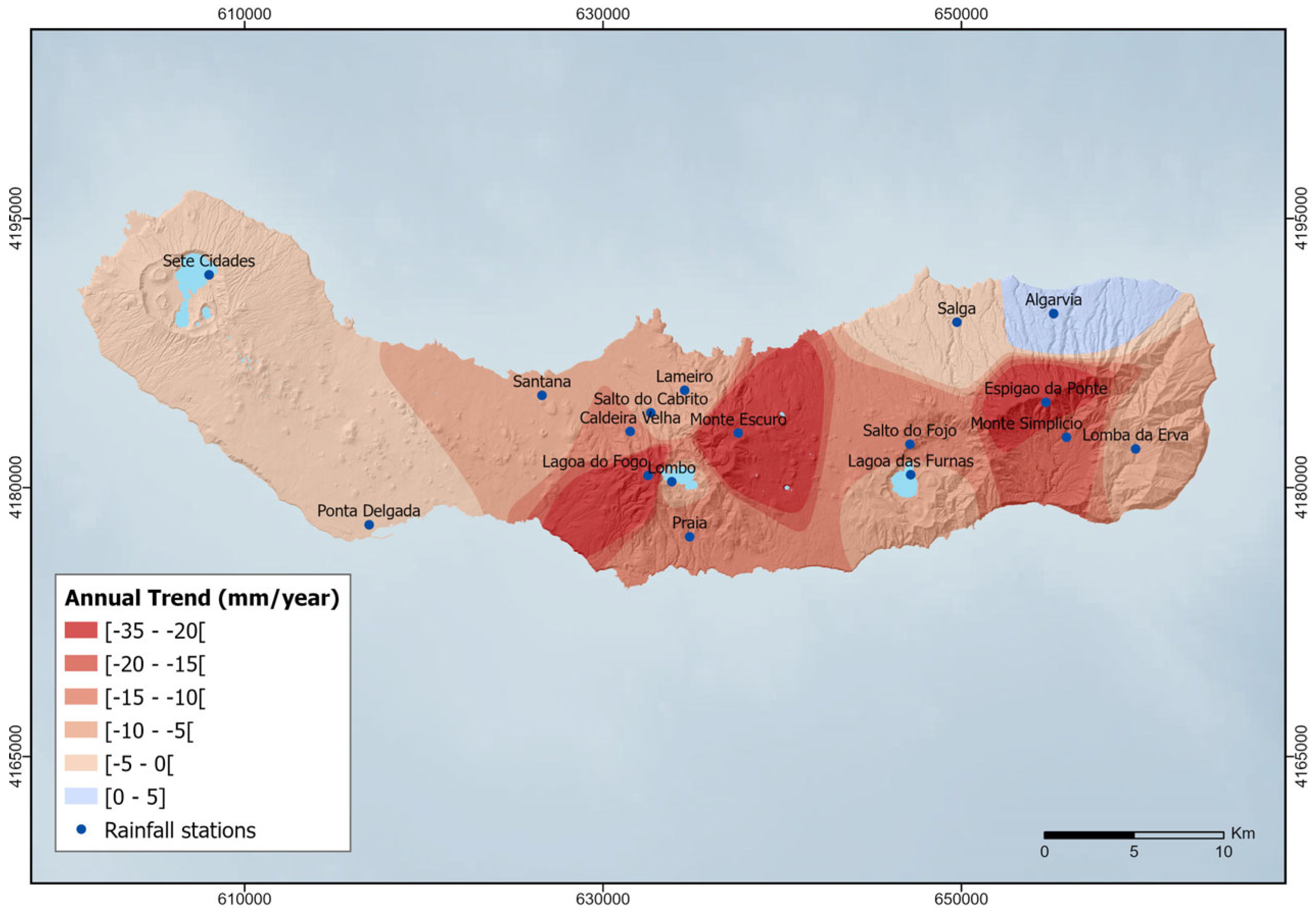
The Mann–Kendall test, paired with Sen’s slope estimator, was used to identify rainfall trends at the 17 stations with data covering the period from 1978/79 to 2019/20. The outcomes, summarised in Table 6, reveal declining trends in rainfall on both the annual and seasonal scales, with autumn exhibiting the most significant decreases. Although visual inspection of the time series and slope estimates indicates decreasing rainfall at many stations, only 5 of the 17 stations showed statistically significant downward annual trends (α ≤ 0.05), highlighting the spatial heterogeneity of rainfall changes across the island. Figure 9 shows the spatial distribution of the annual rainfall trends obtained from the M-K test.
When analysing the rainfall data by clusters, distinct patterns and trends emerge across different regions, underscored by significant changes in rainfall measurements. In Cluster 1, autumn registered the most significant decreases, specifically in Santana (−3.71 mm/year **) and Ponta Delgada (−3.43 mm/year **), pointing to a trend towards drier autumns and an overall reduction in annual rainfall, with Santana being particularly affected. Cluster 2 is characterised by significant reductions, with Monte Simplício showing a notable annual decrease (−19.18 mm/year *). Caldeira Velha exhibits significant decreases in autumn (−6.91 mm/year **), a trend that is also observed at Sete Cidades (−4.19 mm/year *), Lameiro (−4.06 mm/year *), and Salto do Cabrito (−3.96 mm/year *). Moreover, Monte Simplício reveals significant decreases in winter (−7.77 mm/year *) and spring (−5.37 mm/year **), indicating localised environmental changes affecting rainfall patterns. Cluster 3 is highlighted by the severe annual rainfall reduction at Fogo III (−31.57 mm/year ***), along with a considerable decrease at Salto do Fojo (−13.04 mm/year *). This cluster shows the most pronounced rainfall decline across all seasons, especially at Fogo III, with significant reductions in autumn (−12.08 mm/year ***), winter (−10.01 mm/year **), spring (−5.87 mm/year *), and summer (−6.14 mm/year ***). In Cluster 4, Monte Escuro and Espigão da Ponte both show significant annual decreases in rainfall (−25.55 mm/year *** and −21.34 mm/year **, respectively). Monte Escuro also experiences substantial reductions in autumn, spring, and summer (−9.11 mm/year **, −7.10 mm/year *, and −3.57 mm/year *, respectively), while Espigão da Ponte experiences a notable decrease in summer (−4.05 mm/year *). These stations exhibit significant negative variations during summer when compared with other clusters, indicating pronounced seasonal influences on rainfall patterns.

4.5. NAO–Rainfall Relationship

Across the 17 rainfall stations, the Spearman rank correlations reveal a broadly consistent negative association between the Hurrell PC-based NAO index and rainfall, particularly for annual totals and for the autumn season (Table 7).
During autumn, correlations remain predominantly negative and statistically significant at several stations, such as Lomba da Erva (ρ = −0.46, p < 0.01), Monte Simplício (ρ = −0.43, p < 0.01), Salto Fojo (ρ = −0.44, p < 0.01), and Espigão da Ponte (ρ = −0.41, p = 0.01).
By contrast, winter correlations are generally weaker and mostly non-significant (−0.1 to −0.2), while spring and summer correlations are low and spatially inconsistent.
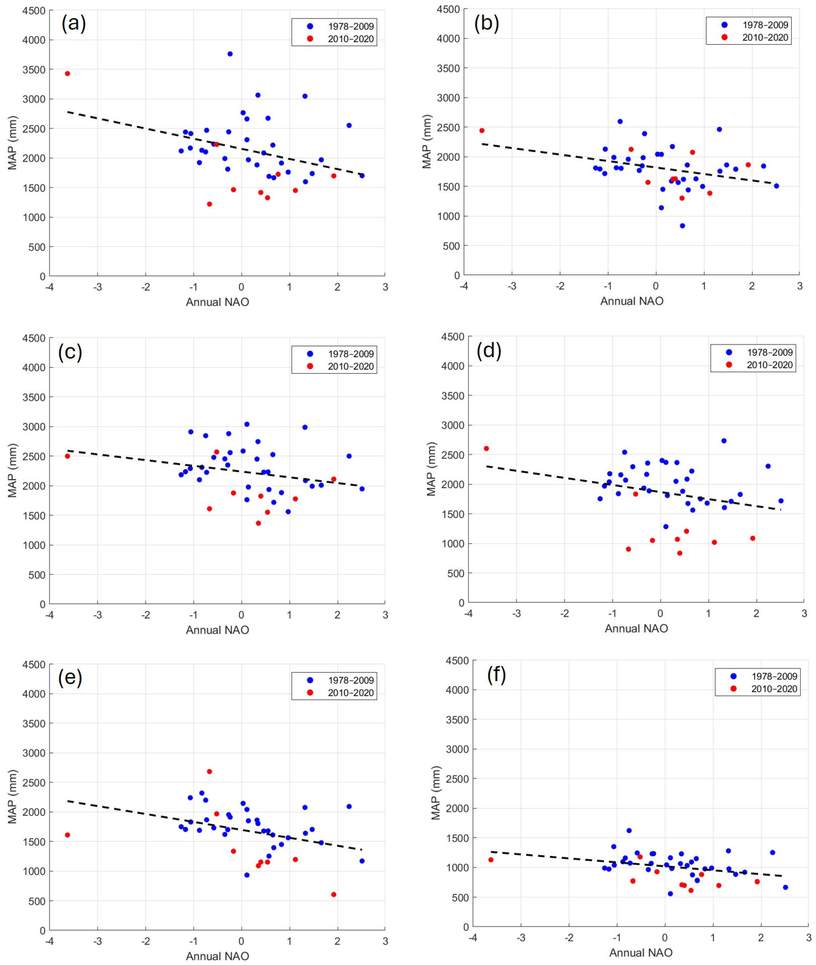
At the annual scale, most stations exhibit negative coefficients, several of which are statistically significant at the 95% confidence level, notably at Salto do Cabrito (ρ = −0.46, p < 0.01), Ponta Delgada (ρ = −0.38, p = 0.01), Sete Cidades (ρ = −0.33, p = 0.03), Monte Simplício (ρ = −0.33, p = 0.04), Lagoa das Furnas (ρ = −0.35, p = 0.02), and Lomba da Erva (ρ = −0.33, p = 0.04).
These six stations are illustrated in Figure 10, which presents scatter plots of annual rainfall versus the NAO index, with data points from the latest sub-dataset (2010–2020) highlighted in red. In general, years with higher NAO values correspond to lower annual rainfall totals. The MAP values in the latest sub-dataset are consistently lower than would be expected.

4.6. Altitude-Rainfall Relationship

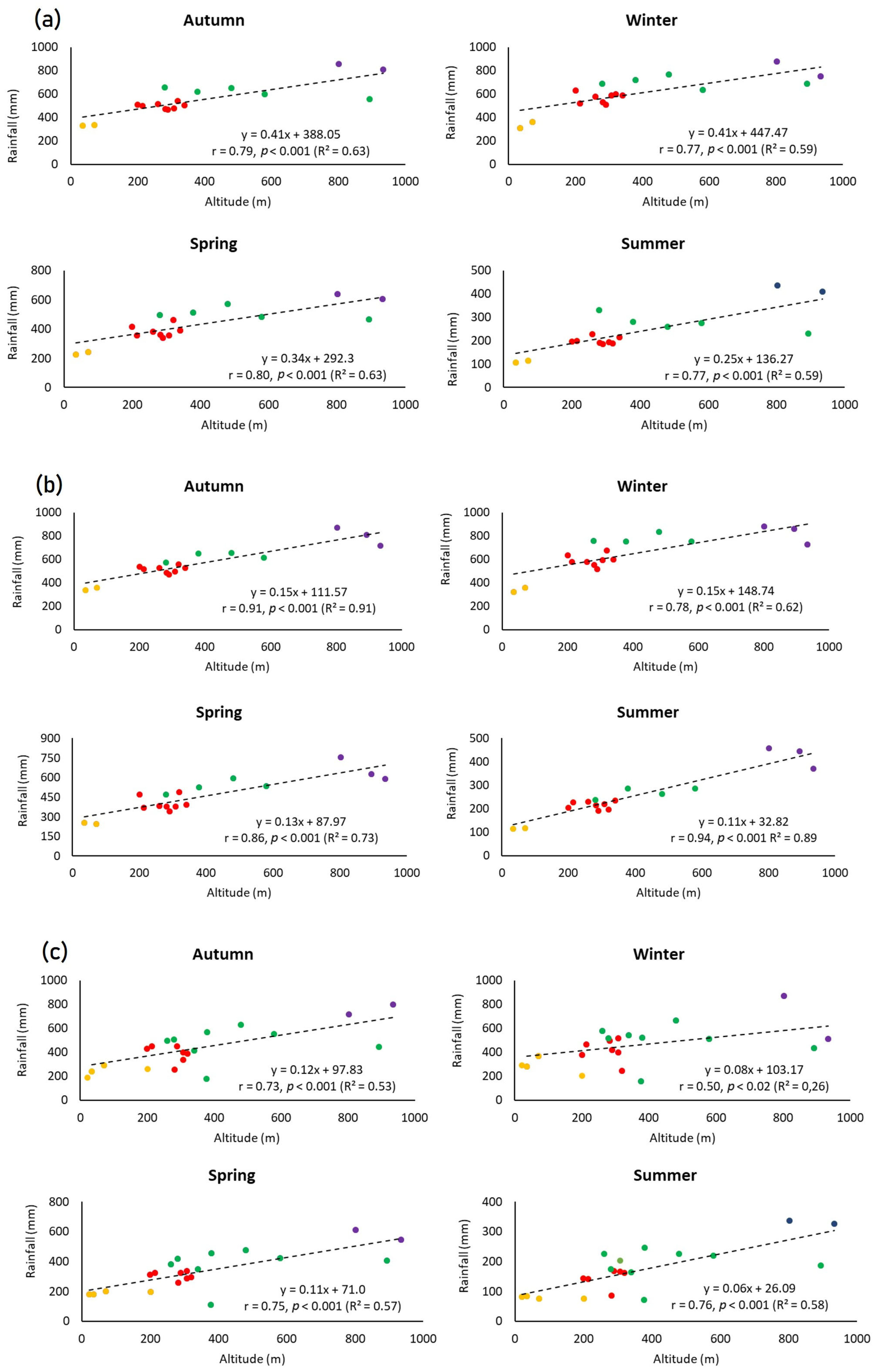
Analysing rainfall’s correlations with altitude provides an insightful examination of the interplay between rainfall metrics and altitude across different climatological periods. As expected, the linear regression analysis, presented in Figure 11 and Figure 12, indicates a strong correlation between the various rainfall variables and altitude, highlighting the influence of altitude on rainfall distribution.
Based on the analysis of the P50 variable (Figure 11), a positive correlation with altitude is observed across all datasets, with stronger relationships occurring in autumn and summer. Winter and spring show a weaker, though still significant, correlation. For the P10 and P90 variables, the results indicate the same behaviour. This observation suggests the presence of additional physiographic factors, such as the existence of central volcanoes, dismantled calderas, and lakes; geological formations’ alignment; ventilation corridors; vegetation; and the orientation of slopes and sea cliffs, which contribute to the variability of the variables beyond that caused by altitude, which can all play significant roles in determining the intensity and distribution of high-magnitude rainfall events.
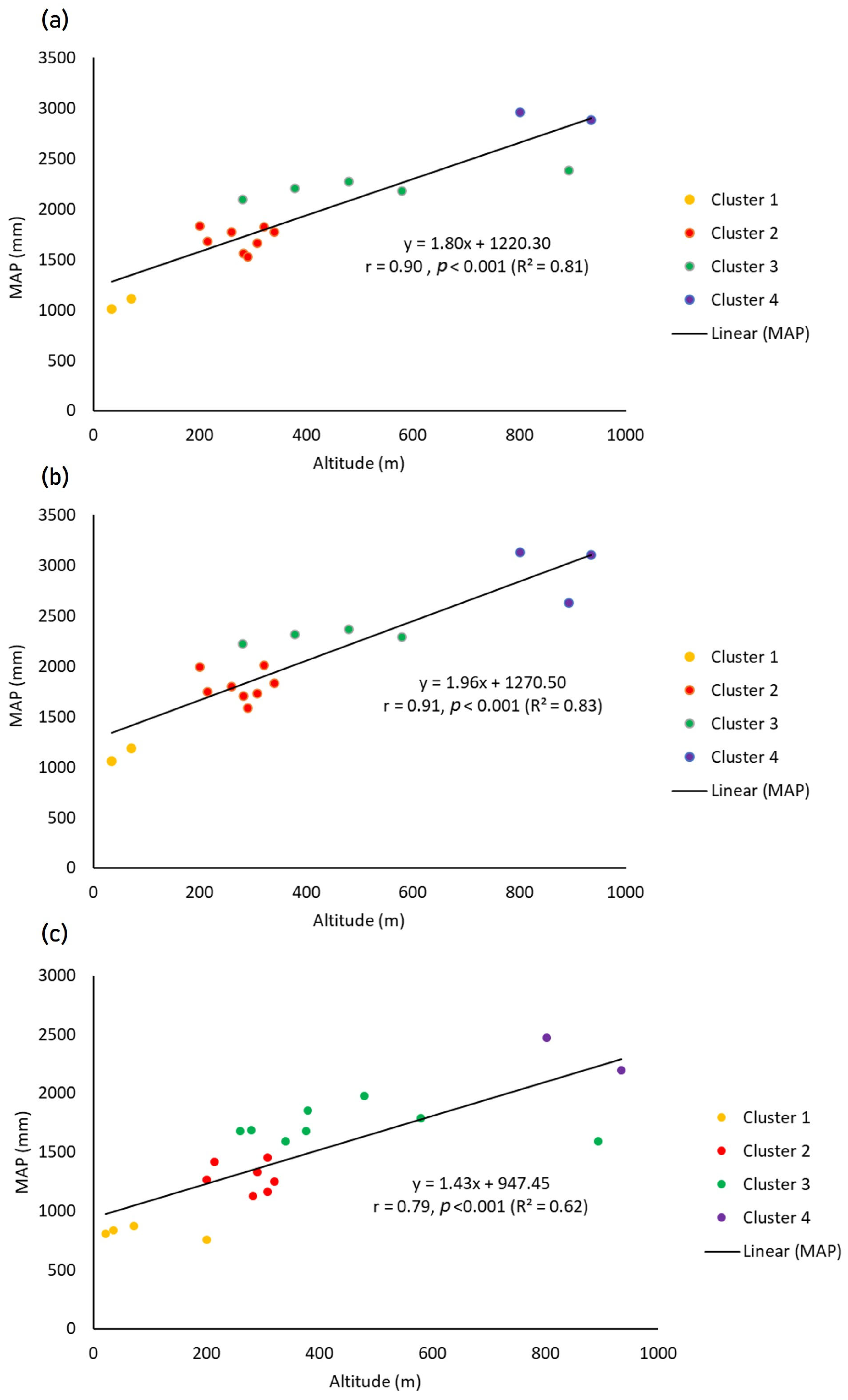
For the full dataset, the correlation coefficient between MAP and altitude is 0.81, indicating a strong positive relationship. The linear regression model suggests that MAP increases by approximately 180 mm for every 100 m of elevation gain (Figure 12a). The spatial distribution of MAP illustrates the altitude influence, with rainfall accumulation ranging from 1120 mm at sea level to 3209 mm at the highest altitude on the island (Figure 13a), reflecting a clear altitudinal gradient in rainfall.
In the oldest sub-dataset, the correlation coefficient increases slightly to 0.83, suggesting an even stronger altitude influence, with a 196 mm increase in MAP per 100 m elevation gain (Figure 12b) and rainfall ranging from 1270 mm at sea level to 3444 mm at the highest points on the island (Figure 13b).
In the latest sub-dataset, the correlation coefficient is 0.62, indicating a slightly weaker but still significant relationship between MAP and altitude. Notably, the rate of increase in rainfall with elevation gain decreases, with MAP rising 144 mm per 100 m altitude gain (Figure 12c). Rainfall values range from 947 mm at sea level to 2537 mm at the highest altitudes (Figure 13c), reflecting an overall reduction in rainfall at higher elevations.
5. Discussion

The cluster analysis, based on rainfall data from the climatological years of 1978/79 to 2019/20, and the two sub-datasets (1978/79 to 2009/10 and 2010/11 to 2019/20), identified four distinct groups of rainfall stations that reflect the spatial and temporal rainfall distribution on São Miguel Island. This analysis provides significant insights into the dynamics of rainfall, highlighting both the constancy and variability of rainfall patterns across the studied period.
The analysis reveals a notable consistency in the clustering of stations over the years, with specific stations being recurrently grouped together, underscoring the stability of rainfall patterns. However, changes in cluster composition were observed when focusing on the oldest and latest sub-datasets, reflecting the variability and evolving rainfall dynamics within the studied timeframe. The greater heterogeneity of rainfall station characteristics within each cluster in the latest sub-dataset, compared with the other periods considered, suggests that longer timeframes—such as the full dataset or the oldest sub-dataset—are more suitable for clustering, yielding more consistent and robust results. In addition, the shorter duration of the latest sub-dataset (10 years) limits the statistical power of trend analyses, making any observed changes during this period more tentative and less conclusive from a climatological standpoint. Furthermore, the shorter duration of the most recent data subset (10 years) limits the statistical power. However, this shorter time window allowed the inclusion of additional rainfall stations that began operating after 2010, thereby improving the spatial coverage and representativeness of the clustering analysis. Similar approaches have been applied in regional studies using shorter time periods to assess emerging climate signals and short-term hydroclimatic variability [77].
Although the clusters are referred to as “homogeneous rainfall regions,” some internal variability remains within each group, as indicated by the coefficients of variation, particularly in the most recent sub-dataset. Therefore, the term “homogeneous” should be interpreted in a statistical sense, referring to the grouping of stations with broadly similar rainfall regimes and temporal behaviour, rather than complete uniformity.
Rainfall stations within each cluster are generally located at similar altitudes, although exceptions indicate that factors other than altitude influence rainfall distribution, as observed in other regions worldwide [78,79]. On São Miguel, the complex volcanic morphology plays a major role in shaping local rainfall patterns. Stations located within or near volcanic calderas, such as Lagoa das Furnas, Fogo, and Sete Cidades, often record higher rainfall totals than nearby stations at comparable altitudes. This is likely explained by the geomorphological setting of these depressions, where steep caldera rims and elevated relief enhance orographic uplift and moisture condensation. Consequently, the clustering results reflect not only the altitudinal gradient but also the combined effects of volcanic topography and local atmospheric circulation on rainfall distribution across the island.
A significant finding of this study is the variability in Mean Annual Rainfall (MAP) across clusters, coupled with evident seasonal variations. These results align with the expected annual rainfall cycle on the island, with higher values typically being recorded in winter and lower values in summer. Seasonal variations in the variables are consistent with the island’s climatic pattern, in which winter is the wettest season and summer is the driest. Seasonal fluctuations in P10, P50, and P90 values align with the island’s climate, with P10 values being relatively uniform across seasons and clusters, while P50 and P90 show important differences, especially during the wettest months. These variables play a crucial role in cluster differentiation.
Temporal analysis comparing the two sub-datasets unveils a decrease in rainfall in the most recent period. Previous long-term studies based on the centennial rainfall series of São Miguel Island indicate that MAP values were higher during the more recent periods of those records. This pattern was demonstrated by Hernández et al. [40] for the period of 1943–2012 and by Cropper and Hanna [39] for the period of 1981–2010. However, the results of this study reveal a reduction in rainfall that was not detected in these earlier long-term analyses, suggesting that the rainfall decline is mainly concentrated in the period after 2010.
Trend analyses for the climatological years of 1978/79–2019/20, using the M–K test and Sen’s slope estimator, indicate predominantly decreasing trends in annual and seasonal rainfall; however, statistically significant declines were only detected at a subset of stations. Autumn displays the most pronounced reductions across multiple stations and clusters, indicating a systemic shift towards drier autumns on São Miguel Island. Cluster-based analysis further reveals spatial variations in these trends. Notably, Cluster 1 experiences a marked decrease in autumn rainfall, particularly in Santana and Ponta Delgada, indicating a shift towards drier conditions. Cluster 2 shows notable reductions in several seasons, with Monte Simplício experiencing significant declines in annual and winter rainfall. Cluster 3, notably at Fogo III, suffers drastic reductions in rainfall across all seasons, likely with severe ecological and hydrological implications. Similarly, Cluster 4, which includes Monte Escuro and Espigão da Ponte, shows significant annual and seasonal rainfall declines. These findings underscore the critical need for understanding regional rainfall trends to mitigate potential negative effects on ecosystems and water resources.
Climate change scenarios for the Azores predict an increase in winter rainfall and a reduction in summer rainfall [80]. However, some of the observed reductions in rainfall, especially during autumn and winter, appear to contrast with these climate projections. Nonetheless, the limited spatial significance of these trends calls for further investigation before definitive conclusions are drawn. Climate change projections suggest that subtropical anticyclones will undergo changes in intensity and location. It is expected that the anticyclones over the North Pacific, South Atlantic, and South Indian Oceans will weaken, while the subtropical anticyclone over the North Atlantic will intensify [81]. The decreasing rainfall trend observed in this study could be linked to this intensification, driven by increased tropospheric static stability resulting from changes in diabatic heating patterns [81]. Additionally, expansion of the Azores High during the 20th century, driven by the increase in greenhouse gas concentrations, has decreased rainfall in winter, a trend that is expected to continue in the coming years with global warming [82]. This expansion also contributes to decreasing rainfall on the Eastern Iberian Peninsula [83].
Across São Miguel, annual rainfall maintains the expected negative association with the PC-based NAO; however, the pronounced drying of the latest sub-dataset occurs even under neutral or negative NAO phases. This suggests that additional climate drivers, such as the East Atlantic pattern, the Scandinavian pattern, or broader North Atlantic SST anomalies, may also be influencing recent rainfall behaviour [84,85]. A more detailed investigation of these teleconnections is therefore warranted to fully understand the observed downward trend.
The obtained results show a strong positive relationship between station altitude and rainfall, with rainfall increasing consistently with altitude. However, the strength of this relationship has decreased in recent years, suggesting that the altitude–rainfall dependency may not be strictly linear and could be modulated by additional factors. This differs from other regions that are influenced by subtropical anticyclones, where rainfall does not always increase with altitude [86,87,88].
Furthermore, the identified clusters and rainfall patterns suggest that there are no clear differences between windward and leeward slopes, unlike in many other regions, where the windward side typically receives more rain [89,90]. The limited orographic contrast between the windward and leeward slopes can be attributed to the island’s small size and its west–east alignment, which offers little resistance to the prevailing winds. These factors, combined with moderate topographic gradients, restrict the development of heavy rain shadow effects.

6. Conclusions

This study explored the spatial and temporal patterns of rainfall on São Miguel Island (Azores) in the period of 1978/79–2019/20. Consistent patterns in rainfall distribution were identified across four clusters, although some changes in cluster composition were observed in the most recent period (2010/11–2019/20). A notable finding was the significant variability in rainfall metrics across different clusters, with each cluster exhibiting distinct Mean Annual Rainfall (MAP) values. Seasonal variations in rainfall distribution were also evident, with higher values typically being recorded in winter and lower values in summer, reflecting the island’s characteristic annual rainfall pattern.
The spatial distribution of rainfall stations within each cluster, relative to altitude, suggests a strong correlation between elevation and rainfall patterns on São Miguel Island. However, some exceptions to this trend were observed, indicating the influence of additional factors beyond altitude. These anomalies, such as stations appearing in unexpected clusters, can be attributed to local geographic or environmental features, including the presence of volcanic calderas.
The trend analysis provided critical insights, indicating decreasing trends in both annual and seasonal rainfall at several locations on the island. However, statistically significant reductions were detected at only a limited number of stations (5 out of 17 at the annual scale). Notably, autumn exhibited the most consistent and significant decrease across several stations and clusters, suggesting a shift towards drier conditions. These findings provide preliminary evidence of changing rainfall patterns on São Miguel Island, while highlighting the need for continued monitoring and long-term datasets to robustly assess climate trends. Given the diverse topographical and climatic conditions across the Azores islands, expanding this analysis to include the entire archipelago would provide a more comprehensive understanding of regional rainfall trends and their potential implications. Across the island, rainfall also maintains the expected negative association with the NAO, particularly in autumn and for annual totals. However, the most recent decade consistently shows lower rainfall even under neutral or negative NAO phases. This suggests that the recent drying trend cannot be explained by the NAO alone and may reflect the influence of additional atmospheric modes over the North Atlantic.
The integration of cluster and trend analysis not only enabled the identification of previously unrecognised rainfall patterns but also introduced a novel methodological approach in the context of the Azores. The identification of homogeneous rainfall regions and the analysis of temporal trends can also support the optimisation of the monitoring network, facilitating the strategic installation and maintenance of rainfall stations in key areas. By revealing evolving climatic dynamics and proposing a replicable methodological model, this work represents a significant advancement in the scientific understanding of climate variability in the Azores and offers practical tools for sustainable land and risk management.

Author Contributions

R.F.S.: conceptualisation, methodology, formal analysis, writing—original draft, and writing—review and editing. R.M.: methodology, supervision, formal analysis, writing—original draft, and writing—review and editing. J.L.Z.: methodology, supervision, formal analysis, writing—original draft, and writing—review and editing. M.F.: methodology, formal analysis, and writing—review and editing. All authors have read and agreed to the published version of the manuscript.

Funding

This work was supported by the Fundação para a Ciência e a Tecnologia (FCT) through the scholarship UI/BD/152207/2021 (DOI: https://doi.org/10.54499/UI/BD/152207/2021). J.L.Z. and M.F. were supported by the Fundação para a Ciência e a Tecnologia (FCT), by the Research Unit UID/00295/2025 (DOI: https://doi.org/10.54499/UID/00295/2025).

Data Availability Statement

Data will be made available on request.

Acknowledgments

The authors are grateful to the Portuguese Institute for Sea and Atmosphere (IPMA) and Direção Regional do Ordenamento do Território e Recursos Hídricos do Governo da Região Autónoma dos Açores (DROTRH-GRAA) for providing the data and information from rainfall stations used in this study.

Conflicts of Interest

The authors declare that they have no known competing financial interests or personal relationships that could have appeared to influence the work reported in this paper.

References

  1. Frich, P.; Alexander, L.V.; Della-Marta, P.; Gleason, B.; Haylock, M.; Klein Tank, A.M.G.; Peterson, T. Observed coherent changes in climatic extremes during the second half of twentieth century. Clim. Res. 2002, 19, 193–212. [Google Scholar] [CrossRef]
  2. Novotny, E.V.; Stefan, H.G. Stream flow in Minnesota: Indicator of climate change. J. Hydrol. 2007, 334, 319–333. [Google Scholar] [CrossRef]
  3. Valdés-Pineda, R.; Pizarro-Tapia, R.; Valdés, J.B.; Diaz, H.F. Analysis of spatio-temporal changes in annual and seasonal rainfall variability in South America-Chile and related ocean–atmosphere circulation patterns. Int. J. Climatol. 2015, 36, 2979–3001. [Google Scholar] [CrossRef]
  4. Lin, G.F.; Chen, L.H. Identification of homogeneous regions for regional frequency analysis using the self-organizing map. J. Hydrol. 2006, 324, 1–9. [Google Scholar] [CrossRef]
  5. Guttman, N.B. The use of L-moments in the determination of regional rainfall climates. J. Clim. 1993, 6, 2309–2325. [Google Scholar] [CrossRef]
  6. Modarres, R.; Sarhadi, A. Statistically-based regionalization of rainfall climates of Iran. Glob. Planet. Change 2011, 75, 67–75. [Google Scholar] [CrossRef]
  7. Machiwal, D.; Dayal, D.; Kumar, S. Long-term rainfall trends and change points in hot and cold arid regions of India. Hydrol. Sci. J. 2017, 62, 1050–1066. [Google Scholar] [CrossRef]
  8. Medina-Cobo, M.T.; García-Marín, A.P.; Estévez, J.; Jiménez-Hornero, F.J.; Ayuso-Muñoz, J.L. Obtaining homogeneous regions by determining the generalized fractal dimensions of validated daily rainfall data sets. Water Resour. Manag. 2017, 31, 2333–2348. [Google Scholar] [CrossRef]
  9. Suhaila, J.; Jemain, A.A. A comparison of the rainfall patterns between stations on the East and the West coasts of Peninsular Malaysia using the smoothing model of rainfall amounts. Meteorol. Appl. 2009, 16, 391–401. [Google Scholar] [CrossRef]
  10. Şen, Z.; Habib, Z. Monthly spatial rainfall correlation functions and interpretations for Turkey. Hydrol. Sci. J. 2001, 46, 525–535. [Google Scholar] [CrossRef]
  11. Sabziparvar, A.A.; Movahedi, S.; Asakereh, H.; Maryanaji, Z.; Masoodian, S.A. Geographical factors affecting variability of rainfall regime in Iran. Theor. Appl. Climatol. 2015, 120, 367–376. [Google Scholar] [CrossRef]
  12. Jebari, S.; Berndtsson, R.; Uvo, C.; Bahri, A. Regionalizing fine time-scale rainfall affected by topography in semi-arid Tunisia. Hydrol. Sci. J. 2009, 52, 1199–1215. [Google Scholar] [CrossRef]
  13. Haines, H.A.; Olley, J.M. The implications of regional variations in rainfall for reconstructing rainfall patterns using tree rings. Hydrol. Process. 2017, 31, 2951–2960. [Google Scholar] [CrossRef]
  14. Lin, G.F.; Chang, M.J.; Wu, J.T. A hybrid statistical downscaling method based on the classification of rainfall patterns. Water Resour. Manag. 2017, 31, 377–401. [Google Scholar] [CrossRef]
  15. Gupta, A.; Kamble, T.; Machiwal, D. Comparison of ordinary and Bayesian kriging techniques in depicting rainfall variability in arid and semi-arid regions of north-west India. Environ. Earth Sci. 2017, 76, 512. [Google Scholar] [CrossRef]
  16. Jackson, I.J.; Weinand, H. Classification of Tropical Rainfall Stations: A Comparison of Clustering Techniques. Int. J. Climatol. 1995, 15, 985–994. [Google Scholar] [CrossRef]
  17. Ward, J.H., Jr. Hierarchical Grouping to Optimize an Objective Function. J. Am. Stat. Assoc. 1963, 58, 236–244. [Google Scholar] [CrossRef]
  18. Masoodian, S.A. An Analysis of Tempo-Spatial Variation or Rainfall in Iran. Ph.D. Thesis, University of Isfahan, Isfahan, Iran, 1998. [Google Scholar]
  19. Domroes, M.; Kaviani, M.; Schaefer, D. An Analysis of Regional and Intra-annual Rainfall Variability over Iran using Multivariate Statistical Methods. Theor. Appl. Climatol. 1998, 61, 151–159. [Google Scholar] [CrossRef]
  20. Unal, Y.; Kindap, T.; Karaca, M. Redefining the climate zones of Turkey using cluster analysis. Int. J. Climatol. 2003, 23, 1045–1055. [Google Scholar] [CrossRef]
  21. Martin, T.N.; Storck, L.; Dourado Neto, D. Simulação Estocástica da Radiação Fotossinteticamente Ativa e da Temperatura do Ar por Diferentes Métodos. Pesqui. Agropecu. Bras. 2007, 42, 1211–1219. [Google Scholar] [CrossRef]
  22. Lyra, G.B.; Oliveira-Júnior, J.F.; Zeri, M. Cluster analysis applied to the spatial and temporal variability of monthly rainfall in Alagoas state, Northeast of Brazil. Int. J. Climatol. 2014, 34, 3546–3558. [Google Scholar] [CrossRef]
  23. Zhang, Q.; Liu, C.; Xu, C.; Xu, Y.; Jiang, T. Observed trends of annual maximum water level and streamflow during past 130 years in the Yangtze River basin, China. J. Hydrol. 2006, 324, 255–265. [Google Scholar] [CrossRef]
  24. Chen, H.; Guo, S.; Xu, C.; Singh, V.P. Historical temporal trends of hydro-climatic variables and runoff response to climate variability and their relevance in water resource management in the Hanjiang basin. J. Hydrol. 2007, 344, 171–184. [Google Scholar] [CrossRef]
  25. Mirabbasi, R.; Ahmadi, F.; Jhajharia, D. Comparison of parametric and non-parametric methods for trend identification in groundwater levels in Sirjan plain aquifer, Iran. Hydrol. Res. 2020, 51, 1455–1477. [Google Scholar] [CrossRef]
  26. Sonali, P.; Nagesh Kumar, D. Review of trend detection methods and their application to detect temperature changes in India. J. Hydrol. 2013, 476, 212–227. [Google Scholar] [CrossRef]
  27. Kendall, S. Time Series; Oxford University Press: New York, NY, USA, 1976. [Google Scholar]
  28. Mann, H.B. Non-Parametric Test Against Trend. Econometrica 1945, 13, 245–259. [Google Scholar] [CrossRef]
  29. Theil, H. A rank-invariant method of linear and polynomial regression analysis. I, II, III. Ned. Akad. Wet. Proc. Ser. A 1950, 53, 386–525. [Google Scholar]
  30. Sen, P.K. Estimates of the regression coefficient based on Kendall’s tau. J. Am. Stat. Assoc. 1968, 63, 1379–1389. [Google Scholar] [CrossRef]
  31. Kumar, S.; Santosh, S. Temporal and Spatial Dynamics of Rainfall in Satluj River Basin, Himachal Pradesh, India. Int. Lett. Chem. Phys. Astron. 2015, 54, 150–165. [Google Scholar] [CrossRef]
  32. Foresti, L.; Pozdnoukhov, A.; Kanevski, M. Data-driven exploration of orographic enhancement of rainfall. Adv. Sci. Res. 2011, 6, 129–135. [Google Scholar] [CrossRef]
  33. Chen, Y.-L.; Feng, J. Numerical Simulations of Airflow and Cloud Distributions over the Windward Side of the Island of Hawaii. Part I: The Effects of Trade Wind Inversion. Mon. Weather Rev. 2001, 129, 1117–1134. [Google Scholar] [CrossRef]
  34. Iqbal, M.J.; Khan, F.; Hameed, S. Influence of Azores High pressure on Middle Eastern rainfall. Theor. Appl. Climatol. 2012, 111, 211–221. [Google Scholar] [CrossRef]
  35. Rashid, S.A.; Iqbal, M.J.; Hussain, M.A. Impact of North-South Shift of Azores High on Summer Rainfall over North West Europe. Int. J. Geosci. 2012, 3, 992–999. [Google Scholar] [CrossRef]
  36. Loo, Y.Y.; Billa, L.; Singh, A. Effect of climate change on seasonal monsoon in Asia and its impact on the variability of monsoon rainfall in Southeast Asia. Geosci. Front. 2014, 6, 817–823. [Google Scholar] [CrossRef]
  37. Santos, F.D.; Valente, M.A.; Miranda, P.M.A.; Aguiar, A.; Azevedo, E.B.; Tomé, A.R.; Coelho, F. Climate change scenarios in the Azores and Madeira islands. World Resour. Rev. 2004, 16, 473–491. [Google Scholar]
  38. De Lima, M.I.P.; Carvalho, S.C.P.; De Lima, J.L.M.P. Investigating Annual and Monthly Trends in Rainfall Structure: An Overview Across Portugal. Nat. Hazards Earth Syst. Sci. 2010, 10, 2429–2440. [Google Scholar] [CrossRef]
  39. Cropper, T.E.; Hanna, E. An analysis of the climate of Macaronesia, 1865–2012. Int. J. Climatol. 2014, 34, 604–622. [Google Scholar] [CrossRef]
  40. Hernández, A.; Kutiel, H.; Trigo, R.M.; Valente, M.A.; Sigró, J.; Cropper, T.; Santo, F.E. New Azores archipelago daily rainfall dataset and its links with large-scale modes of climate variability. Int. J. Climatol. 2016, 36, 4439–4454. [Google Scholar] [CrossRef]
  41. Marques, R.; Zêzere, J.; Trigo, R.; Gaspar, J.; Trigo, I. Rainfall patterns and critical values associated with landslides in Povoação County (São Miguel Island, Azores): Relationships with the North Atlantic Oscillation. Hydrol. Process. 2008, 22, 478–494. [Google Scholar] [CrossRef]
  42. Queiroz, G. Vulcão das Sete Cidades (S. Miguel, Açores)—História Eruptiva e Avaliação do Hazard. Ph.D. Thesis, University of the Azores, Azores, Portugal, 1997. [Google Scholar]
  43. Queiroz, G.; Gaspar, J.L.; Guest, J.E.; Gomes, A.; Almeida, M.H. Eruptive History and Evolution of Sete Cidades Volcano, São Miguel Island, Azores. In Volcanic Geology of São Miguel Island (Azores Archipelago); Gaspar, J.L., Guest, J.E., Duncan, A.M., Barriga, F.J.A.S., Chester, D.K., Eds.; Memoirs; The Geological Society of London: London, UK, 2015; Volume 44, pp. 87–104. [Google Scholar]
  44. Wallenstein, N. Estudo da História Recente e do Comportamento Eruptivo do Vulcão do Fogo (S. Miguel, Açores). Avaliação preliminar do Hazard. Ph.D. Thesis, University of the Azores, Azores, Portugal, 1999. [Google Scholar]
  45. Wallenstein, N.; Duncan, A.; Guest, J.E.; Almeida, M.H. Eruptive History of Fogo Volcano, São Miguel, Azores. In Volcanic Geology of São Miguel Island (Azores Archipelago); Gaspar, J.L., Guest, J.E., Duncan, A.M., Barriga, F.J.A.S., Chester, D.K., Eds.; Memoirs; The Geological Society of London: London, UK, 2015; Volume 44, pp. 105–123. [Google Scholar]
  46. Guest, J.E.; Gaspar, J.L.; Cole, P.D.; Queiroz, G.; Duncan, A.M.; Wallenstein, N.; Ferreira, T.; Pacheco, J.M. Volcanic geology of Furnas Volcano, São Miguel, Azores. J. Volcanol. Geotherm. Res. 1999, 92, 1–29. [Google Scholar] [CrossRef]
  47. Guest, J.E.; Pacheco, J.M.; Cole, P.D.; Duncan, A.M.; Wallenstein, N.; Queiroz, G.; Gaspar, J.L.; Ferreira, T. The volcanic history of Furnas volcano, São Miguel, Azores. In Volcanic Geology of São Miguel Island (Azores Archipelago); Gaspar, J.L., Guest, J.E., Duncan, A.M., Barriga, F.J.A.S., Chester, D.K., Eds.; Memoirs; The Geological Society of London: London, UK, 2015; Volume 44, pp. 125–134. [Google Scholar]
  48. Ferreira, T. Caracterização da Actividade Vulcânica da ilha de S. Miguel (Açores): Vulcanismo Basáltico Recente e Zonas de Desgaseificação. Avaliação de Riscos. Ph.D. Thesis, University of the Azores, Azores, Portugal, 2000. [Google Scholar]
  49. Ferreira, T.; Gomes, A.; Gaspar, J.L.; Guest, J. Distribution and significance of basaltic eruptive centres: São Miguel, Azores. In Volcanic Geology of São Miguel Island (Azores Archipelago); Gaspar, J.L., Guest, J.E., Duncan, A.M., Barriga, F.J.A.S., Chester, D.K., Eds.; Memoirs; The Geological Society of London: London, UK, 2015; Volume 44, pp. 135–146. [Google Scholar]
  50. Booth, B.; Croasdale, R.; Walker, G.P.L. A quantitative study of five thousand years of volcanism on S. Miguel, Azores. Philos. Trans. R. Soc. Lond. 1978, 228, 271–319. [Google Scholar]
  51. Duncan, A.M.; Guest, J.E.; Wallenstein, N.; Chester, D.K. The oldest volcanic complexes of São Miguel, Azores: Nordeste and Povoação. In Volcanic Geology of São Miguel Island (Azores Archipelago); Gaspar, J.L., Guest, J.E., Duncan, A.M., Barriga, F.J.A.S., Chester, D.K., Eds.; Memoirs; The Geological Society of London: London, UK, 2015; Volume 44, pp. 147–153. [Google Scholar]
  52. Azevedo, E.B. Condicionantes Dinâmicas do Clima no Arquipélago dos Açores: Elementos para o Seu Estudo. Açoreana 2001, 9, 309–317. [Google Scholar]
  53. Hurrell, J.W.; Kushnir, Y.; Ottersen, G.; Visbeck, M. An Overview of the North Atlantic Oscillation. In The North Atlantic Oscillation: Climatic Significance and Environmental Impact; Hurrell, J.W., Kushnir, Y., Ottersen, G., Visbeck, M., Eds.; American Geophysical Union: Washington, DC, USA, 2003. [Google Scholar]
  54. Carvalho, F.S.; Meirelles, M.G.; Henriques, D.V.; Navarro, P.V.; Vasconcelos, H.C. Climate Change and the Increase of Extreme Events in Azores. In Handbook of Human and Planetary Health; Climate Change Management; Springer: Berlin/Heidelberg, Germany, 2022; pp. 349–365. [Google Scholar]
  55. Chazarra, A.; Baceló, A.M.; Pires, V.; Cunha, S.; Silva, A.; Marques, J.; Carvalho, F.; Mendes, M.; Neto, J.; Mendes, L. Climate Atlas of the Archipelagos of the Canary Islands, Madeira and the Azores; Department of the State Meteorological Agency of Spain and Department of Meteorology and Climatology of the Institute of Meteorology: Lisbon, Portugal, 2011. [Google Scholar]
  56. Azevedo, E.B. Modelação do Clima Insular à Escala Local—Modelo CIELO aplicado à Ilha Terceira. Ph.D. Thesis, University of the Azores, Azores, Portugal, 1996. [Google Scholar]
  57. Fernandes, J. Caracterização Climática das ilhas de São Miguel e Santa Maria com Base no Modelo CIELO; Internship Report; University of the Azores: Azores, Portugal, 2004. [Google Scholar]
  58. Azevedo, E.B.; Pereira, L.S.; Itier, B. Modeling the Local Climate in Island Environments: Water Balance Applications. Agric. Water Manag. 1999, 40, 393–403. [Google Scholar] [CrossRef]
  59. Brito, R.S. São Miguel—A Ilha Verde. Estudo Geográfico (1950–2000), 2nd ed.; Instituto de Alta Cultura, Centro de Estudos Geográficos: Lisboa, Portugal, 2004. [Google Scholar]
  60. Rodrigues, R. Hidrologia de Ilhas Vulcânicas; Dissertação para Obtenção do grau de Especialista; Laboratório Nacional de Engenharia Civil: Lisboa, Portugal, 1995. [Google Scholar]
  61. Rodrigues, R. Avaliação das Disponibilidades Hídricas da Ilha de São Miguel (Açores); Rel. 217/92—NHHF; Laboratório Nacional de Engenharia Civil: Lisboa, Portugal, 1992. [Google Scholar]
  62. Royston, P. An extension of Shapiro and Wilk’s W test for normality to large samples. Appl. Stat. 1982, 31, 115–124. [Google Scholar] [CrossRef]
  63. Deheuvels, P.A. Kolmogorov–Smirnov type test for independence and multivariate samples. Rev. Roum. Math. Pure. Appl. 1981, 26, 213–226. [Google Scholar]
  64. Alexandersson, H.; Moberg, A. Homogenization of Swedish temperature data. Part I: Homogeneity test for linear trends. Int. J. Climatol. 1997, 17, 25–34. [Google Scholar] [CrossRef]
  65. Buishand, T.A. Some methods for testing the homogeneity of rainfall records. J. Hydrol. 1982, 58, 11–27. [Google Scholar] [CrossRef]
  66. Pettitt, A.N. A non-parametric approach to the change-point problem. Appl. Stat. 1979, 28, 126–135. [Google Scholar] [CrossRef]
  67. Von Neumann, J. Distribution of the ratio of the mean square successive difference to the variance. Ann. Math. Stat. 1941, 12, 367–395. [Google Scholar] [CrossRef]
  68. Wijngaard, J.B.; Klein-Tank, A.M.G.; Können, G.P. Homogeneity of 20th century European daily temperature and rainfall series. Int. J. Climatol. 2003, 23, 679–692. [Google Scholar] [CrossRef]
  69. Everitt, B.S.; Dunn, G. Applied Multivariate Analysis; Edward Arnold: London, UK, 1991. [Google Scholar]
  70. Wang, J.; Chen, J.; Shen, P.; Guan, X.; Liu, X.; Massari, C.; Yong, B. Regional-Scale Intelligent Optimization and Topography Impact in Restoring Global Rainfall Data Gaps. Commun. Earth Environ. 2025, 6, 671. [Google Scholar] [CrossRef]
  71. Tsubo, M.; Walker, S.; Hensley, M. Quantifying Risk for Water Harvesting under Semi-Arid Conditions: Part I. Rainfall Intensity Generation. Agric. Water Manag. 2005, 76, 77–93. [Google Scholar] [CrossRef]
  72. Mazvimavi, D. Investigating Changes over Time of Annual Rainfall in Zimbabwe. Hydrol. Earth Syst. Sci. 2010, 14, 2671–2679. [Google Scholar] [CrossRef]
  73. World Meteorological Organization. Guide to Climatological Practices, 2nd ed.; WMO: Geneva, Switzerland, 2018; 139p. [Google Scholar]
  74. Sa’adi, Z.; Shahid, S.; Ismail, T.; Chung, E.S.; Wang, X.J. Trends analysis of rainfall and rainfall extremes in Sarawak, Malaysia using modified Mann–Kendall test. Meteorol. Atmos. Phys. 2019, 131, 263–277. [Google Scholar] [CrossRef]
  75. Wilks, D.S. Statistical Methods in the Atmospheric Sciences, 4th ed.; Academic Press: Cambridge, MA, USA, 2020. [Google Scholar]
  76. Lund, R.B.; Beaulieu, C.; Killick, R.; Lu, Q.; Shi, X. Good practices and common pitfalls in climate time series changepoint techniques: A review. J. Clim. 2023, 36, 8041–8057. [Google Scholar] [CrossRef]
  77. Spinoni, J.; Naumann, G.; Vogt, J.V.; Barbosa, P. The biggest drought events in Europe from 1950 to 2012. J. Hydrol. Reg. Stud. 2015, 3, 509–524. [Google Scholar] [CrossRef]
  78. Rianna, M.; Montesarchio, V.; Napolitano, F.; Ubertini, L. A Preliminary Analysis of Rainfall Spatial Distribution at Catchment Scale. AIP Conf. Proc. 2015, 1648, 190009. [Google Scholar] [CrossRef]
  79. Mahindawansha, A.; Jost, M.; Gassmann, M. Spatial and Temporal Variations of Stable Isotopes in Rainfall in the Mountainous Region, North Hesse. Water 2022, 14, 3910. [Google Scholar] [CrossRef]
  80. Programa Regional para as Alterações Climáticas (PRAC). Decreto Legislativo Regional n.º 30/2019/A; Diário da República n.º 229/2019, Série I; Assembleia Legislativa da Região Autónoma dos Açores: Ponta Delgada, Portugal, 2019. [Google Scholar]
  81. He, C.; Wu, B.; Zou, L.; Zhou, T. Responses of the Summertime Subtropical Anticyclones to Global Warming. J. Clim. 2017, 30, 6465–6479. [Google Scholar] [CrossRef]
  82. Cresswell-Clay, N.; Ummenhofer, C.C.; Thatcher, D.L.; Wanamaker, A.D.; Denniston, R.F.; Asmerom, Y.; Polyak, V.J. Twentieth-Century Azores High Expansion Unprecedented in the Past 1200 Years. Nat. Geosci. 2022, 15, 548–553. [Google Scholar] [CrossRef]
  83. Miró, J.J.; Estrela, M.J.; Corell, D.; Gómez, I.; Luna, M.Y. Rainfall and Drought Trends (1952–2021) in a Key Hydrological Recharge Area of the Eastern Iberian Peninsula. Atmos. Res. 2023, 286, 106695. [Google Scholar] [CrossRef]
  84. Rodrigo, F.S. Exploring Combined Influences of Seasonal East Atlantic (EA) and North Atlantic Oscillation (NAO) on the Temperature-Precipitation Relationship in the Iberian Peninsula. Geosciences 2021, 11, 211. [Google Scholar] [CrossRef]
  85. Comas-Bru, L.; McDermott, F. Impacts of the EA and SCA patterns on the European twentieth century NAO–winter climate relationship. Q. J. R. Meteorol. Soc. 2014, 140, 354–363. [Google Scholar] [CrossRef]
  86. Rodwell, M.J.; Hoskins, B.J. Subtropical Anticyclones and Summer Monsoons. J. Clim. 2001, 14, 3192–3211. [Google Scholar] [CrossRef]
  87. Lopes, S. Clima e Ordenamento do Território no Funchal. Ph.D. Thesis, University of Lisbon, Lisbon, Portugal, 2015. [Google Scholar]
  88. Söllheim, Á.L.L.; Suarez, P.M.; Hernández, F.G. The Digital Climate Atlas of the Canary Islands: A Tool to Improve Knowledge of Climate and Temperature and Rainfall Trends in the Atlantic Islands. Clim. Serv. 2024, 34, 100487. [Google Scholar] [CrossRef]
  89. Peñate, I.; Rodríguez, G.; Cianca, A.; Martín-González, J.M. Scaling Properties of Rainfall and Desert Dust in the Canary Islands. Nonlinear Process. Geophys. 2013, 20, 1079–1094. [Google Scholar] [CrossRef]
  90. Van Den Hende, C.; Nyssen, J.; Van Schaeybroeck, B.; Van Vooren, S.; Van Ginderachter, M.; Termonia, P. Analysis of Rain-Shadows in the Ethiopian Mountains Using Climatological Model Data. Clim. Dyn. 2021, 56, 1663–1679. [Google Scholar] [CrossRef]
Figure 1. Geographic location (a), altitude, and morphostructural units (b) of São Miguel Island: 1—Sete Cidades Volcano; 2—Picos Fissural Volcanic System; 3—Fogo Volcano; 4—Congro Fissural Volcanic System; 5—Furnas Volcano; 6—Povoacão Volcano; 7—Nordeste Volcanic Complex.
Climate 13 00238 g001
Figure 2. Mean sea-level pressure (hPa) over the North Atlantic in January (top) and July (bottom). The Azores region is highlighted with a white dotted rectangle. The panels were generated by the authors using Climate Data Operators (CDOs; https://code.mpimet.mpg.de/projects/cdo, accessed on 20 May 2025) to compute average fields and Panoply (https://www.giss.nasa.gov/tools/panoply/, accessed on 20 May 2025) for map visualisation. Data source: Copernicus Climate Data Store—ERA5 daily statistics.
Climate 13 00238 g002
Figure 3. Average monthly rainfall (blue bars) and average monthly temperature (orange line) at the Ponta Delgada meteorological station for the period of 1981–2010 (climate normal data from the Portuguese Institute for Sea and Atmosphere, IPMA, IP).
Climate 13 00238 g003
Figure 4. Geographic locations of rainfall stations (numbers correspond to stations listed in Table 1).
Climate 13 00238 g004
Figure 5. Dendrogram with rainfall stations and their clusters for (a) the full dataset, (b) the oldest sub-dataset, and (c) the latest sub-dataset.
Climate 13 00238 g005
Figure 6. Silhouette Coefficient for different numbers of clusters (k) for the full dataset, the oldest sub-dataset, and the latest sub-dataset.
Climate 13 00238 g006
Figure 7. Hypsometric map illustrating the distribution of rainfall station clusters for (a) the full dataset, (b) the oldest sub-dataset, and (c) the latest sub-dataset.
Climate 13 00238 g007
Figure 8. Evolution of the Mean Annual Rainfall recorded between the climatological years 1978/79 and 2019/20 at the rainfall stations of Santana (Cluster 1), Caldeira Velha (Cluster 2), Salto do Fojo (Cluster 3), and Monte Escuro (Cluster 4).
Climate 13 00238 g008
Figure 9. Spatial distribution of the annual rainfall trends (mm/year), determined by the M–K test.
Climate 13 00238 g009
Figure 10. Scatterplots of MAP versus annual NAO index for (a) Lagoa das Furnas, (b) Sete Cidades, (c) Lomba da Erva, (d) Monte Simplício, (e) Salto do Cabrito, and (f) Ponta Delgada. The trend line is dotted.
Climate 13 00238 g010
Figure 11. Correlation of the P50 variable with altitude across clusters in every season for (a) the full dataset, (b) the oldest sub-dataset, and (c) the latest sub-dataset. The trend line is dotted.
Climate 13 00238 g011
Figure 12. Correlation of Mean Annual Rainfall (MAP) with altitude across clusters for (a) the full dataset, (b) the oldest sub-dataset, and (c) the latest sub-dataset. The trend line is dotted.
Climate 13 00238 g012
Figure 13. Spatial distribution of Mean Annual Rainfall (MAP) and the locations of rainfall station clusters for (a) the full dataset, (b) the oldest sub-dataset, and (c) the latest sub-dataset.
Climate 13 00238 g013
Table 1. Rainfall stations used in the analysis and descriptive statistics for the annual time series.
Nr.Rainfall StationAltitude (m)Data PeriodNr. of Days p ≥ 1 mmAnnual Rainfall (mm)
MAPMin.Max.Standard Deviation
1Mosteiros212010/11–2019/20106838.2540.51147.8189.8
2Sete Cidades2601978/79–2019/201581797.5833.62596.3353.7
3Candelária2012010/11–2019/20109753.6614.71191.0452.9
4Capelas3772010/11–2019/201401679.91358.72188.7286.6
5Santana711978/79–2019/201061135.3671.11801.1267.1
6Ponta Delgada201978/79–2019/201201006.1558.41620.9218.5
7Chã da Macela3082010/11–2019/201371160.4569.01548.2263.9
8Caldeira Velha2831978/79–2019/201261562.9386.62340.3418.0
9Salto do Cabrito2141978/79–2019/201351675.6606.12682.8407.8
10Lameiro3081978/79–2019/201471666.4985.42364.0318.3
11Fogo III8931978/79–2019/201722384.5964.74620.8714.1
12Lombo5801978/79–2019/201562183.91116.03606.4556.0
13Praia2001978/79–2019/201401831.2928.33070.1520.6
14Monte Escuro8021978/79–2019/201932963.01996.34186.0547.1
15Salga2901978/79–2019/201361524.1814.12340.4326.6
16Algarvia3401978/79–2019/201411777.2961.32659.7387.9
17Salto do Fojo4801978/79–2019/201352276.81393.43049.2417.2
18Lagoa das Furnas2801978/79–2019/201512127.41219.03762.4557.0
19Monte Simplício3201978/79–2019/201301849.4834.52734.0485.3
20Espigão da Ponte9341978/79–2019/202012888.01567.58393.01181.3
21Lomba da Erva3791978/79–2019/201612224.11366.63039.3419.7
Table 2. Statistics for the Shapiro–Wilk and Kolmogorov–Smirnov normality tests, applied to the annual rainfall time series. The results in bold indicate which series have normal distributions at a 5% significance level. The classification of the series is based on the results of the homogeneity tests.
Nr.Rainfall StationData PeriodNormality TestsClassification Based on Homogeneity Tests
Shapiro–WilkKolmogorov–Smirnov
2Sete Cidades1978/79–2019/200.4160.671Useful
5Santana1978/79–2019/200.3590.720Useful
6Ponta Delgada1978/79–2019/200.4350.885Useful
8Caldeira Velha1978/79–2019/200.0940.277Useful
9Salto do Cabrito1978/79–2019/200.5670.574Useful
10Lameiro1978/79–2019/200.5300.660Useful
11Fogo III1978/79–2019/200.0120.326Doubtful
12Lombo1978/79–2019/200.8280.978Useful
13Praia1978/79–2019/200.4700.756Useful
14Monte Escuro1978/79–2019/200.3290.972Useful
15Salga1978/79–2019/200.5550.785Useful
16Algarvia1978/79–2019/200.9900.996Useful
17Salto do Fojo1978/79–2019/200.4980.928Useful
18Lagoa das Furnas1978/79–2019/200.0570.697Useful
19Monte Simplício1978/79–2019/200.1220.609Doubtful
20Espigão da Ponte1978/79–2019/200.0000.061Doubtful
21Lomba da Erva1978/79–2019/200.7930.977Useful
Table 3. Mean values (mm) of rainfall variables for each cluster during the climatological years of 1978/79–2019/20, 1978/79–2009/10, and 2010/11–2019/20.
DatasetFull DatasetOldest Sub-DatasetLatest Sub-Dataset
Climatological Years1978/79–2019/201978/79–2009/102010/11–2019/20
VariableCluster 1Cluster 2Cluster 3Cluster 4Cluster 1Cluster 2Cluster 3Cluster 4Cluster 1Cluster 2Cluster 3Cluster 4
P10 Autumn210.8332.0405.1547.4252.6369.5448.4581.0147.9216.5333.3445.6
P50 Autumn331.4497.5616.5833.8346.5513.9624.0799.4244.3388.5514.2760.4
P90 Autumn435.6699.4864.41158.1449.6712.0878.01133.0364.2562.4710.5977.4
P10 Winter194.8313.4443.9553.4234.0398.3525.4593.7104.5215.6232.8405.5
P50 Winter335.0567.9700.3814.2339.9591.5773.1823.6285.7417.7547.3692.3
P90 Winter559.9855.01173.71365.2577.5874.21146.51384.5387.0665.8809.41023.7
P10 Spring128.9215.8301.6422.6131.1233.9298.5426.8106.6182.3281.1379.2
P50 Spring232.8382.5506.0621.0250.8400.9531.7656.8190.4305.5406.1578.4
P90 Spring394.7635.3888.81075.8396.1640.9889.21061.7285.7425.6619.7694.0
P10 Summer54.2115.7150.0296.471.3135.5179.2320.545.287.3112.8211.2
P50 Summer111.2199.4276.1423.2115.1214.6268.8424.279.5153.1205.1331.9
P90 Summer207.8321.8417.4595.7212.9329.8394.7581.2163.7208.8341.7437.6
MAP1070.61710.62239.42925.51124.21800.92301.02954.4835.81292.61762.02335.3
Table 4. Coefficient of variation (CV) of rainfall variables for each cluster during the climatological years of 1978/79–2019/20, 1978/79–2009/10, and 2010/11–2019/20.
DatasetFull DatasetOldest Sub-DatasetLatest Sub-Dataset
Climatological Years1978/79–2019/201978/79–2009/102010/11–2019/20
VariableCluster 1Cluster 2Cluster 3Cluster 4Cluster 1Cluster 2Cluster 3Cluster 4Cluster 1Cluster 2Cluster 3Cluster 4
P10 Autumn1.0%18.5%12.8%8.6%4.4%9.2%7.0%6.1%22.9%32.9%21.2%5.4%
P50 Autumn1.2%5.0%6.8%4.0%3.7%5.7%6.1%9.7%17.9%18.1%13.4%7.5%
P90 Autumn12.8%9.3%10.1%5.2%11.5%8.0%3.6%9.8%6.6%19.0%12.4%6.6%
P10 Winter7.5%18.0%7.6%20.9%2.8%12.1%9.0%11.5%22.6%21.1%36.3%30.2%
P50 Winter10.6%7.4%6.8%11.2%7.1%8.2%5.2%10.4%23.5%21.8%12.8%37.0%
P90 Winter7.4%10.1%5.6%0.4%11.4%12.5%2.7%5.4%13.5%14.4%10.9%25.9%
P10 Spring5.8%11.4%7.9%11.0%8.1%20.4%4.8%15.4%22.6%35.8%17.7%1.6%
P50 Spring5.1%10.4%8.1%3.9%2.3%12.7%9.8%13.5%5.5%8.5%11.9%8.2%
P90 Spring4.5%8.9%4.0%9.6%5.0%10.8%2.2%11.9%11.0%8.5%17.6%9.5%
P10 Summer6.9%19.3%13.6%17.3%12.6%11.5%13.3%18.3%25.1%26.2%17.9%8.0%
P50 Summer4.9%7.0%13.4%4.5%1.2%7.6%8.6%11.2%5.0%23.4%14.1%2.4%
P90 Summer14.5%9.0%12.8%0.3%17.5%7.7%5.6%9.5%27.3%19.4%23.4%10.7%
MAP8.5%7.2%4.4%1.8%8.2%7.9%2.5%9.4%8.1%9.5%7.9%8.3%
Table 5. Rate of change in the value of rainfall variables between the oldest and latest sub-datasets.
VariableCluster 1Cluster 2Cluster 3Cluster 4
P10 Autumn−41.4%−41.4%−25.7%−23.3%
P50 Autumn−29.5%−24.4%−17.6%−4.9%
P90 Autumn−19.0%−21.0%−19.1%−13.7%
P10 Winter−55.3%−45.9%−55.7%−31.7%
P50 Winter−15.9%−29.4%−29.2%−15.9%
P90 Winter−33.0%−23.8%−29.4%−26.1%
P10 Spring−18.7%−22.1%−5.8%−11.2%
P50 Spring−24.1%−23.8%−23.6%−11.9%
P90 Spring−27.9%−33.6%−30.3%−34.6%
P10 Summer−36.6%−35.6%−37.1%−34.1%
P50 Summer−30.9%−28.7%−23.7%−21.8%
P90 Summer−23.1%−36.7%−13.4%−24.7%
MAP−25.7%−28.2%−23.4%−21.0%
Table 6. Sen’s slope estimator of the annual and seasonal rainfall trends (numerical values, mm/year) and respective levels of significance according to the M–K Test.
ClusterRainfall StationQAnnualQAutmunQWinterQSpringQSummer
1Ponta Delgada−3.70−3.43 **−1.13−0.730.20
Santana−7.19−3.71 **−1.56−0.95−0.57
2Caldeira Velha−12.21−6.91 **−1.78−3.04−3.15 *
Salga−1.88−1.150.500.10−0.64
Monte Simplício−19.18 *−4.27−7.77 *−5.37 *−1.16
Praia−10.75−2.86−3.16−3.79 *−0.66
Lameiro−7.05−4.06 *−0.40−1.21−0.35
Salto Cabrito−7.91−3.96 *−2.53−1.23−2.30 *
Sete Cidades−0.81−4.19 *−0.340.131.06
Algarvia2.68−1.64−1.220.400.25
3Lombo−9.70−1.98−6.39−1.54−0.11
Lagoa Furnas−9.44−4.17 *−2.16−3.25−1.05
Fogo III−31.57 ***−12.08 ***−10.01 **−5.87 *−6.14 ***
Lomba da Erva−9.05−3.21−2.87−3.09−0.66
Salto Fojo−13.04 *−3.36−4.23−3.18−1.32
4Monte Escuro−25.55 ***−9.11 **−5.12−7.10 *−3.57 *
Espigão da Ponte−21.34 **−2.95−6.75−5.02−4.05 *
*** trend at α = 0.001 level of significance; ** trend at α = 0.01 level of significance; * trend at α = 0.05 level of significance.
Table 7. Spearman rank correlation coefficients between annual and seasonal rainfall and the Hurrell PC-based NAO index. Values in bold indicate statistical significance at p < 0.05.
Rainfall StationAnnualAutumnWinterSpringSummer
Lagoa Furnas−0.35−0.26−0.14−0.100.27
Lombo−0.26−0.28−0.130.140.06
Santana−0.27−0.28−0.060.120.44
Sete Cidades−0.33−0.24−0.110.290.23
Algarvia−0.24−0.38−0.110.150.28
Caldeira Velha−0.30−0.18−0.160.020.29
Espigão da Ponte0.09−0.41−0.090.110.38
Fogo III−0.12−0.13−0.260.100.37
Lameiro−0.28−0.25−0.170.160.40
Lomba da Erva−0.33−0.46−0.280.160.04
Monte Escuro−0.030.03−0.220.010.61
Monte Simplício−0.33−0.43−0.200.020.05
Praia−0.06−0.28−0.120.130.29
Salga−0.16−0.20−0.080.260.22
Salto Cabrito−0.46−0.35−0.230.080.38
Salto Fojo−0.30−0.44−0.170.040.28
Ponta Delgada−0.38−0.18−0.170.050.32
Disclaimer/Publisher’s Note: The statements, opinions and data contained in all publications are solely those of the individual author(s) and contributor(s) and not of MDPI and/or the editor(s). MDPI and/or the editor(s) disclaim responsibility for any injury to people or property resulting from any ideas, methods, instructions or products referred to in the content.