Article

Climatology of Synoptic Non-Gaussian Meteorological Anomalies in the Northern Hemisphere during 1979–2018

1
Institute of Monitoring of Climatic and Ecological Systems, Siberian Branch of Russian Academy of Sciences, Tomsk 634055, Russia
2
Department of Meteorology and Climatology, Faculty of Geology and Geography, National Research Tomsk State University, Tomsk 634050, Russia
3
The Center for Research and Invention, Rabochaya, 18, Veliky Novgorod 173008, Russia
4
School of Mathematics and Statistics, The Open University, Milton Keynes MK7 6AA, UK
*
Author to whom correspondence should be addressed.
Climate 2024, 12(1), 8; https://doi.org/10.3390/cli12010008
Submission received: 13 December 2023 / Revised: 5 January 2024 / Accepted: 8 January 2024 / Published: 12 January 2024
(This article belongs to the Special Issue The Importance of Long Climate Records)

Abstract

:
The analysis of spatial and temporal variability in the number of non-Gaussian extreme anomalies of climatic parameters was carried out for both the initial time series and synoptic variability in the troposphere of the Northern Hemisphere over the period 1979–2018, based on ERA-Interim reanalysis data. There are predominantly three types of empirical distribution densities at 850 hPa, each characterizing the processes of advective and convective heat transfer. At the beginning of the 21st century, compared to the end of the 20th century, there was an increase in the number of anomalies in vertical wind speed and specific humidity for the Northern Hemisphere. Additionally, there is an increase in the number of zonal wind speed anomalies in the low and middle latitudes. Regions with the maximum number of anomalies are primarily located over the continents, while for vertical wind speed anomalies, they are predominantly over the oceans. The application of R/S analysis and multifractal analysis has established that the identified tendencies (which are persistent processes) will continue in the identified regions. The time series of non-Gaussian anomalies (both initial and synoptic scales) exhibit a long-term memory of approximately four years, and synoptic extreme anomalies were found to be more predictable.

1. Introduction

Against the backdrop of global changes in surface air temperature in the late 20th to early 21st centuries [1], there has been an increase in meteorological parameter anomalies, as well as a rise in the frequency and severity of dangerous and unfavorable natural phenomena (such as heat and cold waves, heavy rain and snow, squally winds, floods, droughts, and others) [2,3,4].
One common method for studying the climatology of anomalies involves analyzing the properties of their probability distribution function (PDF), identifying the variability of its characteristics across different regions over long-time intervals.
According to [2,3,4,5,6,7,8], the current climate change impacts not only the mean values of meteorological parameters (for example, surface temperature) but also their positive and negative anomalies, although the frequency and magnitude of these changes vary regionally.
Extreme events are often associated with changes in large-scale atmospheric circulation processes. For instance, changes in anomalies, as well as their PDFs, may be associated with advective and convective transfer of heat and moisture [9]. Some climate model calculations suggest that the decreased meridional temperature gradient resulting from Arctic amplification can lead to reduced surface temperature variance in mid-latitudes [1,10]. Moreover, according to [11], the maximal meridional transfer of air masses was observed at the beginning of the 21st century (compared to the 20th century). This tendency, along with a poleward shift in jet streams, may lead to an increase in cold temperature extremes [12,13]. For example, several anomalously cold winters were observed during 2001–2010 in some regions of Northern Eurasia [14,15].
The atmospheric processes mentioned above have a strong influence on the asymmetry of meteorological variable distributions, particularly temperature [12,13,16,17,18]. In general, atmospheric variables do not exhibit Gaussian PDFs, as the atmosphere is a complex, nonlinear system with several inherent asymmetries, such as the rotation of the Earth, uneven insolation, and the changing partial pressure of water vapor with temperature [18]. Each meteorological variable has its individual PDF shape, which can be modified under the mean state of the climate [19,20,21]. For example, Ref. [16] used a clustering algorithm to classify five types of air temperature PDFs over North America. In [22], it is demonstrated that under climate warming, an increase in the positive long tail shift in the temperature distribution would result in a smaller increase in the frequency of extreme warm events than if the distribution was Gaussian. Regarding short tails, Ref. [23] notes that there is a larger increase in the number of days exceeding a fixed threshold compared to shifting a Gaussian distribution by the same amount. Additionally, skewness has been found to be important for climate change studies, as short-tailed distributions are much more sensitive to a change in the mean than long-tailed distributions [22,24,25].
It was revealed that different time scales of atmospheric processes (high-frequency processes with a period less than 2 days, synoptic processes with a period of 2–7 days, and low-frequency processes with a period of 10–30 days) could make different contributions of nonlinear interactions to the total dynamics. Some studies find deviations from Gaussianity even on synoptic time scales [17,26,27,28]. According to [12], the processes of synoptic temperature advection and the eddy circulation are important for the investigation of relationships between anomalous temperature and velocity. In addition, nonzero PDF temperature skewness may occur from the eddy covariance [29]. This result is in contrast to [10] who concluded synoptic near-surface temperature variations in mid-latitudes are statistically indistinguishable from Gaussian. However, significant deviations from the normal distribution were revealed in the regions of baroclinic disturbances generation over the western parts of ocean in the mid-latitudes [27,28] and the maximal deviations were marked when the anomalies exceeded 3σ [22]. A leading role in the formation of areas with extreme “warm” temperatures around the globe belongs to advection, storm tracks, jet streams, centers of atmospheric action and atmospheric blockings [12,15,30,31,32].
Thus, non-Gaussian geophysical processes, which occur at various intensities and have distinct temporal and spatial scales, lead to the formation of anomalies in basic climatic variables. To analyze these non-Gaussian time series and obtain characteristics of their structure and trends, fractal and wavelet analysis algorithms are used [33,34,35]. These algorithms are robust methods for detecting deterministic chaos, long-term memory, and cycles. In the context of climate change, identifying atmospheric disturbances associated with these processes, as well as the challenge of understanding their long-term variability (or predictability), is not only of high interest but also a labor-intensive goal.
In the studies mentioned earlier, which are primarily focused on air temperature, one element of the analysis involves identifying the reasons for the variability of the first moments/cumulants of the anomaly PDF: mean, variance, skewness coefficient, and kurtosis coefficient (which is much less used). Their climatology is also analyzed. The existence of one-sided heavy tails, or the predominant influence of one, is indicated by a significant skewness coefficient, while a significant kurtosis coefficient suggests that the PDF has two heavy tails. In cases where the PDF has one mode and small deformations/perturbations, using the first moments is sufficient to construct the PDF model. However, determining anomaly thresholds based solely on these moments can lead to large errors. This is because each moment is calculated based on the entire range of anomaly values, making the identification of subranges a difficult task. Additional challenges arise with multimodal distributions; in such cases, the first four moments/cumulants cannot classify the type of this PDF, nor allow for the construction of the corresponding distribution model. To address the issue of identifying threshold values for non-Gaussian anomaly intervals, comparing the empirical PDF with the Gaussian model is, in our opinion, a more straightforward approach; however, its reliability will depend on the sample’s length. According to [30], for PDF anomalies with heavy long tails, in contrast to short tails, one can expect more stable predicted dynamics, which this study estimates using R/S and multifractal analysis. The distinction of the approach proposed in this study lies in the classification of PDF types and in determining intervals for anomalies of the main meteorological variables (not limited to temperature). Moreover, it is also crucial that we identify the long-term nonlinear variability of anomalies based not only on their initial time series, but also on a sample with a synoptic time scale.
In this study, we assess the spatial and temporal distributions of non-Gaussian anomalies in climatic parameters across the Northern Hemisphere from 1979 to 2018, and determine the characteristics and tendencies of time series, including variability at the synoptic scale.
The paper is organized as follows: Section 2 presents the datasets and describes the methodology used. Section 3 details the results of the spatio-temporal analysis of the number of non-Gaussian extreme anomalies and their persistence estimates. In Section 4, we discuss the obtained results, comparing them with those of other researchers, and consider possible factors contributing to the revealed variability. The conclusion, along with the limitations and future directions of this research, are briefly summarized in Section 5.

2. Materials and Methods

Our research was conducted in the troposphere of the Northern Hemisphere, focusing on the 850 hPa and 500 hPa isobaric layers, which correspond to the heights of the boundary layer and the middle troposphere, respectively. It is based on the initial time series of meteorological parameters from 6-h ERA-Interim reanalysis data [36], featuring a spatial resolution of 1.125° × 1.125° for the period 1979–2018. Additionally, we extracted synoptic scale variability—specifically 2–7 days, representing vortex circulation of the atmosphere (cyclones/anticyclones)—from the reanalysis data using a bandpass filter. This filter exhibits an attenuation of 25 dB in the low-frequency absorption band and 40 dB in the high-frequency area [28]. Based on the Hamming weight window, it is a non-recursive filter with a finite impulse response and zero phase shift.
Then, we derived time series of the following meteorological parameter anomalies from the initial time series (TS) and from the time series of synoptic variability (SV): air temperature (t′), specific air humidity (q′), wind speed components (zonal—u′, meridional—v′ and vertical—ω′) and geopotential (Φ′). Specific humidity is the mass of water vapour per kilogram of moist air (kg/kg). The total mass of moist air is the sum of the dry air, water vapour, cloud liquid, cloud ice, rain and falling snow (https://codes.ecmwf.int/grib/param-db/?id=133 (accessed on 1 January 2024)).
It was taken that an anomaly is a dimensionless quantity x′(t, m) = (X(t, m) −μ(y(t),m))/σm, representing the deviation of the variable X(t,m) from the mean value μ(y(t),m) for a season (m = 1, …, 4) for each year (y lies in the interval [1979, …, 2018]) and normalized to the standard deviation (σm), σ m 2 = X t , m μ y ( t ) , m 2 ¯ . The standard deviation estimate is calculated from the unbiased (sample adjusted) variance estimate. The overbar means the averaging of the squared deviations over the time interval. The variable of μ(y(t),m) has seasonal and interannual variability, and σm has seasonal variability. The applied approach makes it possible to reduce the nonlinear interannual variability X(t,m) and to normalize the deviation from the mean value to a single value over the entire time interval σm. Further m indices were omitted.
The following characteristics were used in the calculations N a = N x t < a , where −7.5 ≤ a ≤ 7.5, in the area of negative anomalies (aN), as N x t < a , where −7.5 ≤ a < 0, in the area of positive anomalies (aP), as N + x t > a , 0 < a ≤ 7.5. These characteristics were used to calculate the PDF, in addition to the tendencies in extreme positive and negative anomalies. The choice of a range was based on Refs [16,23], where non-Gaussian anomalies were also studied.
To obtain correct estimates over the territory, the averaging of N или N + was carried out with a weight, corresponding to the part of the reanalysis cell area (scell). For example,
N = 1 S λ , φ N λ , φ s c e l l λ , φ , S = λ , φ s c e l l λ , φ ,
where λ—node longitude and φ—node latitude.
Since N is a cumulative sum, we can obtain the empirical probability distribution density (WE) of a random variable x t from the calculation of the N derivative with respect to a.
We consider processes with the Gaussian distribution (WG) and non-Gaussian (empirical) distribution (WE) with (a) skewness W E a W E a ; (b) «heavy» or «fat» tails, i.e., for |a|>>1 the inequalities W E a W G a or W E a W G a . Processes that described by probability density with multimode distribution were not considered.
Boundaries of range for non-Gaussian anomalies (aN и aP) were determined based on the condition of the multiple kurtosis (more than a twice extreme events) of empirical probability distribution ( P E ) above the Gaussian probability distribution ( P G ) for the same variable in the extreme values area a:
P E a < a N P G a < a N = a N W E a d a a N W G a d a > 2 and P E a > a P P G a > a P = a P W E a d a a P   W G a d a > 2
The algorithm for determining aN и aP, which satisfies Condition (2), begins its search from the border of a range. The identified values of aN и aP enable us to distinguish between Gaussian and non-Gaussian event ranges. Consequently, we can identify the characteristics of extreme anomalies (non-Gaussian anomalies) within the ranges [−7.5, aN] U [aP, 7.5]. We analyze only these extreme anomalies further, both for TS, as SV.
The number of extreme events corresponds to the number of 6 h (based on Era Interim data) periods where the anomaly a value exceeded the threshold values aN or aP (number of measurements~1.46 × 10⁴).
If we compare WE(a) and WG(a) for the condition WE(a) > WG(a), we can identify the main types of distributions:
1.
Type A, when WE(a) values are close to normal distribution:
W E a W G a
2.
Type B, when the exceedance of empirical distribution values occurs in the negative or positive parts of the range, and the skewness coefficient value in distributions of this type will be significant:
W E a > W G a , a > a P or W E a > W G a , a < a N
3.
Type C, when the WE(a) values exceed WG(a) simultaneously in the negative and positive parts of the range, and the kurtosis coefficient value in distributions of this type will be significant:
W E a > W G a , a < a N a > a P
The number of measurements is determined for the null hypothesis (WE(a) = WG(a)) test.
Trends of N or N + were estimated based on the change in the average values in anomaly number over the following time intervals: 1979–1998 and 1999–2018.
Interannual variability of anomalies x y ( t ) , persistence and trend resistance of changes were estimated with the Hurst parameter (H), determined by the method of R/S analysis [37]:
E R n σ n = C n H , n ,
where R—range of accumulated deviations of first values from the mean value of the time series, σ—standard deviation, E—mathematical expectation, n—length of time series sample; C—a constant.
If H > 0.5, time series are called persistent (retain the existing trend), that is, they have long-term memory effects and, therefore, they are trend-resistant and predictable. When H ≈ 0.5, the trend is not clearly pronounced (it corresponds to “white” noise), and and at lower H values the process is an antipersistence, i.e., any trend tends to change by the opposite one, the forecasting is difficult [33,37]. It has been noted that the Hurst values for natural processes are often grouped near the values of H ≈ 0.72–0.73. The error of H determination depends on the length of time intervals, and for short time series, the Hurst parameter of natural processes will occur in the area of “white” noise [38]. Therefore, to analyze areas with anomalous natural processes, the range of “white” noise was given as 0.3–0.7.
Non-stationary processes, where the Hurst exponent (H) varies with time, are termed multifractal. In such cases, the process is characterized by a multifractal spectrum of singularity, denoted as H(t) [39]. The number of fractals can be determined by counting the local Hölder parameters using the multiple-scale analysis method, specifically the ‘wtmm’ procedure from the Matlab software (MATLAB and Statistics Toolbox Release 2016b, The MathWorks, Inc., Natick, MA, USA). To estimate long-term memory, the length of the time interval (measured in years) is divided by the number of fractals identified for that interval.
The statistical significance of the obtained results for the field (in terms of spatial distribution) was estimated using the false discovery rate (FDR) method, specifically the BY01 algorithm from [40]. This approach is necessary because the null hypothesis, formulated as the normality of the PDF of random field values, can be erroneously rejected at several points due to statistical regularities. This can lead to the mistaken identification of structural features that appear to have a sufficiently large spatial scale.
The statistical significance of the derived estimates was determined by a two-tailed null hypothesis t-test at the 0.05 significance level.
In order to derive statistically significant estimates of the interannual variability in rare events (WE ≈ 10−4), the procedure of N averaging over a surface section (box) was applied, including the following spatial dimensions of the box: ~1000 km in the zonal direction and ~500 km in the meridional direction. Although this procedure can lead to a degradation in spatial resolution, it allows us to reduce the number of gaps in time series, and, hence, to stabilize the characteristics of interannual variability.
All used abbreviations are given in the Abbreviations Section.

3. Results

3.1. Types of Probability Distribution Densities

The type of PDF anomalies for each parameter depends on various factors such as atmospheric processes, season, and region [9,31]. To identify the distribution types, the PDFs were calculated for each reanalysis node within the following latitudinal zones: low—0–30° N, medium—31–60° N and high—61–90° N. Three PDF types were distinguished for all the considered parameters and their anomalies. These types of distribution are presented in Figure 1 (for 500 hPa as an example): A, B and C for the whole hemisphere, as well as for its three latitude zones. Here, we provide the PDF types, whose distribution curves are the most representative for each selected type.
The WE(a) distribution is predominantly single mode/unimodal. Despite the WE(a) insignificant differences in the latitudinal zones, the PDF type is retained (Figure 1).
The distribution density curve of Type A presumably can describe the anomalies of air temperature and wind components at 850 hPa, which means that this type can characterize the processes of advective heat transfer in the boundary layer. For other cases, Type A can describe the processes associated with horizontal air motions at the isobaric level in the troposphere (Figure 1a, Table 1).
In Figure 1b, the Type B distribution with positive (or negative) skewness, typical for q′, t′; Φ′ for TS (~48–53% in the middle troposphere), is presented, while for SV, Type B is observed only for Φ′ and u′ (34–37% in the middle troposphere). Thus, in the initial time series, Type B can represent the processes of heat and moisture transfer that are dependent on the geopotential field, whereas at the synoptic time scale, this type pertains solely to processes associated with zonal air transfer at the isobaric level.
The third Type C, where the WE(a) values exceed the WG(a) values both in the positive and negative areas, can presumably describe the horizontal (meridional) and vertical wind speed components for TS (21–33% in the middle troposphere). For a synoptic time scale, Type C characterizes the convective transfer of heat and moisture (57–63%). It should be noted that the most common type of empirical PDF for anomalies for TS is Type B, and for SV, it is Type C, which is probably due to the predominant contribution of q′ and t′ anomalies to the total number of anomalies. Thus, we can observe the changes in the PDF types for these anomalies after filtering the initial time series.
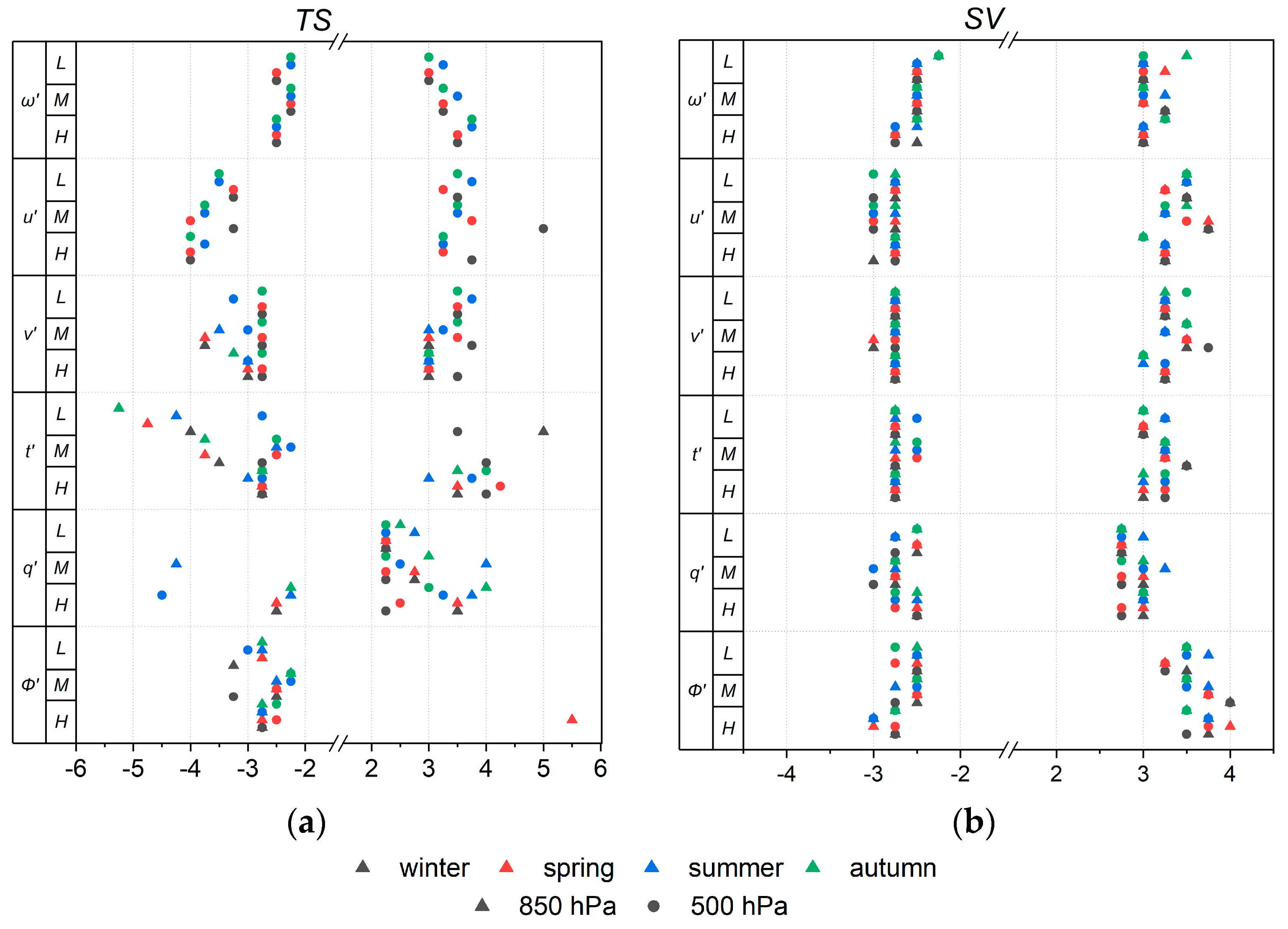
From Figure 2a, it can be observed that the negative TS anomalies are in the interval aN ∈ [−5.25, −2.25], and the positive ones are in the interval aP ∈ [2.25, 5.5]. For SV anomalies, the width of range is twice as small: aN ∈ [−3, −2.25] и aP ∈ [2.75, 4] (Figure 2b). Thus, we determined the interval threshold values for the extreme event PDFs with 0.25 σ accuracy.
The aN and aP boundaries of the TS area are the most constant for the ω′ anomalies, while for t′ and q′, the variability of the boundaries is the highest. For SV, the greatest boundary variability is observed only for aP for Φ′, u′ and v′. These changes are predominantly revealed in the middle latitudes of the Northern Hemisphere. In addition, according to Figure 2, there is a positive skewness in the PDF of anomalies for TS, and negative skewness for SV.
We distinguished three types of PDFs for the initial time series (selected for specified latitudinal zones): (1) Type A—distribution close to Gaussian (t′, u′ and v′—in the boundary layer; u′ and Φ′—in the middle troposphere); (2) Type B—distribution with positive/negative skewness (q′ and Φ′ in the boundary layer; q′, Φ′, t′—in the middle troposphere); (3) Type C—a distribution with a significant kurtosis value and with significant exceedance of PDF values over the Gaussian in the area of negative and positive values (ω′, v′). In the case of SV, we observed changes in the t′ and q′ PDF types to Type C that prevailed for meteorological value anomalies in the boundary layer (~60% of cases). However, at the regional scale, there may be some peculiarities.
Thus, based on the obtained results, we were able to clearly identify the boundaries for non-Gaussian anomalies only for SV: aN = −2.5 and aP = 3. As for TS, the threshold values should be calculated for each considered parameter.

3.2. Spatiotemporal Variability in the Anomalies of Climatic Parameters in the Northern Hemisphere

One of the goals of this study was to evaluate and analyze those anomalies that were previously identified in extreme areas ( a   a N ) ( a   a P ) (Figure 2). Therefore, only anomalies with PDFs corresponding to Types B and C were considered in further analysis (Table 1).
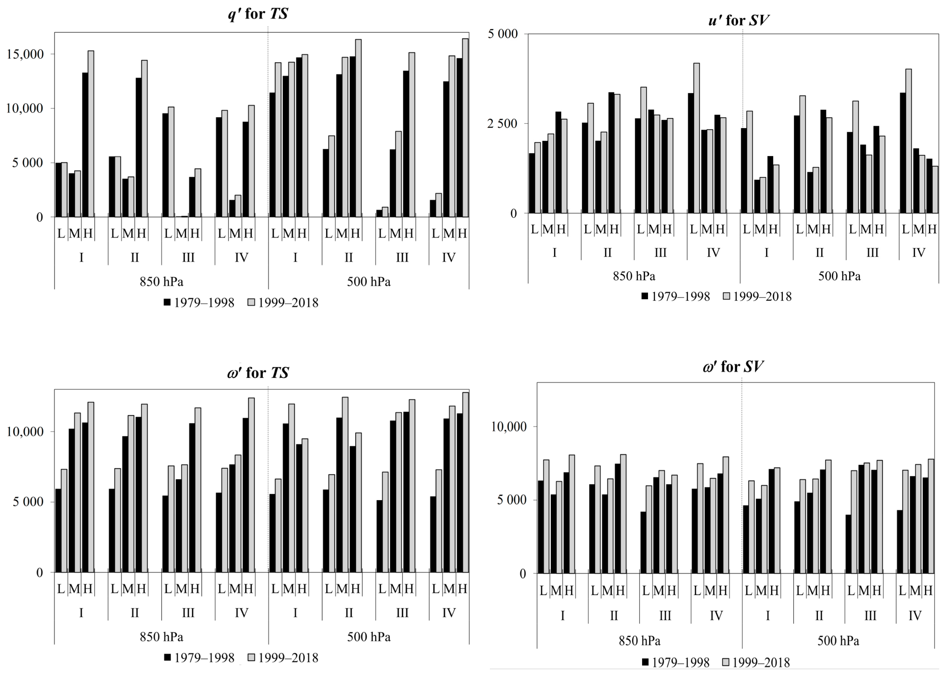
A comparative analysis of the number of anomalies (N) within the previously identified boundaries of non-Gaussian anomalies across two-time intervals (1979–1998 and 1999–2019) revealed the following features. Generally, at the beginning of the 21st century, for both synoptic and initial time scales, N(q′) and N(ω′) predominantly increase in the middle troposphere (as illustrated in Figure 3). The maximum changes are observed in the high latitudes. However, the situation differs for anomalies of the zonal wind speed component at the synoptic time scale. At the beginning of the 21st century, N(u′) increases in the low latitudes in all seasons and in the mid-latitudes during winter and spring. In contrast, in the high latitudes, there is a general decrease in N(u′).
The above results in temporal variability describe the tendencies for the globe as a whole. Further, we will focus on the analysis of the spatial distribution of anomaly numbers of climatic parameters (Figure 4 and Figure 5). The results of the analysis are given for the previously identified PDF type: for N(q′)—Type B for TS, N(u′)—Type B for SV and N(ω′)—Type C for TS and SV.
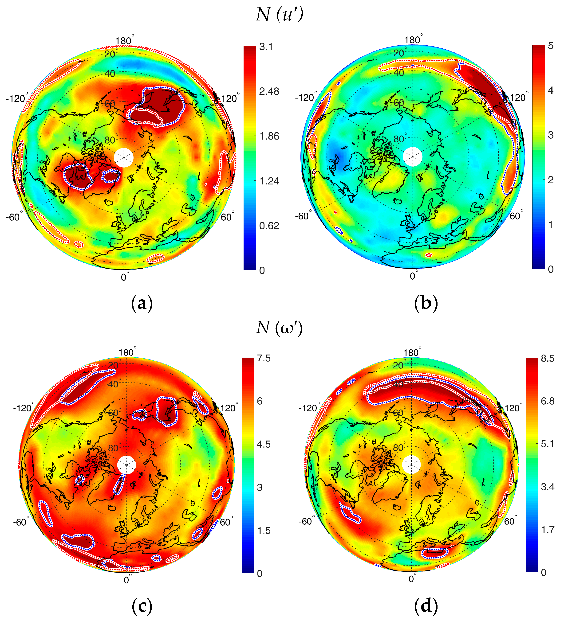
Regions with the maximum number of q′ at 850 hPa for TS in winter are revealed in the high and the middle latitudes of Siberia, the Far East, North America, and North Africa (Figure 4a). As a rule, the anomalies are positive, which indicates the positive PDF skewness. In summer, the maximum N ( q ) is observed in the low latitudes of the Pacific Ocean that can be associated with the region of the El Niño phenomenon influence, and N + ( q ) in southern Africa and in south-western parts of Eurasia (Figure 4b). Moreover, in summer, the region with N + ( q ) is observed to be on the coasts of the Arctic Ocean in Russia.
Regions with maximum N(ω′) at 850 hPa for TS in winter are observed in the middle latitudes of the Pacific and Atlantic oceans (the Gulf Stream and the Kuroshio currents, subtropical gyres and baroclinity zones) (Figure 4c). On the other hand, N (ω′) dominates in the regions mentioned above. The main regions of the N(ω′) maximum for TS in summer, in general, coincide with these in winter (Figure 4d).
A specific feature of the spatial distribution of N(u′) for SV during winter is the location of zones with maximum values at the ocean–land boundary in the northeastern parts of Eurasia, North America, and near Greenland (as shown in Figure 5a). In summer, these regions shift to the low latitudes of the Pacific Ocean (Figure 5b).
In winter, the maximum values of N(ω′) for SV in the Pacific Ocean, as revealed in Figure 5c, become lower than those for TS (Figure 4c), and regions with high values in the Atlantic Ocean completely disappear. Regions with N(ω′) are also observed in the low latitudes of the Northern Hemisphere. In summer, the situation is quite similar; the number of anomalies generally decreases (Figure 5d). However, regions with anomalies in the middle latitudes of the Pacific and Atlantic Oceans are observed for both TS and SV.

3.3. Persistence Estimates of Climatic Parameter Anomalies

The characteristics of interannual variability in anomalies x y ( t ) , the persistence and trend resistance of their changes were estimated based on the Hurst parameter (H) [37]. As it was mentioned earlier (in the “Section 2”, when H > 0.5, the observed tendency remains constant, that is, the time series is persistent, and the H values for natural processes are often grouped around values of 0.72–0.73. Therefore, in further analysis, special attention is paid to the values of H > 0.72 (Table 2, Figure 6, Figure 7 and Figure 8).
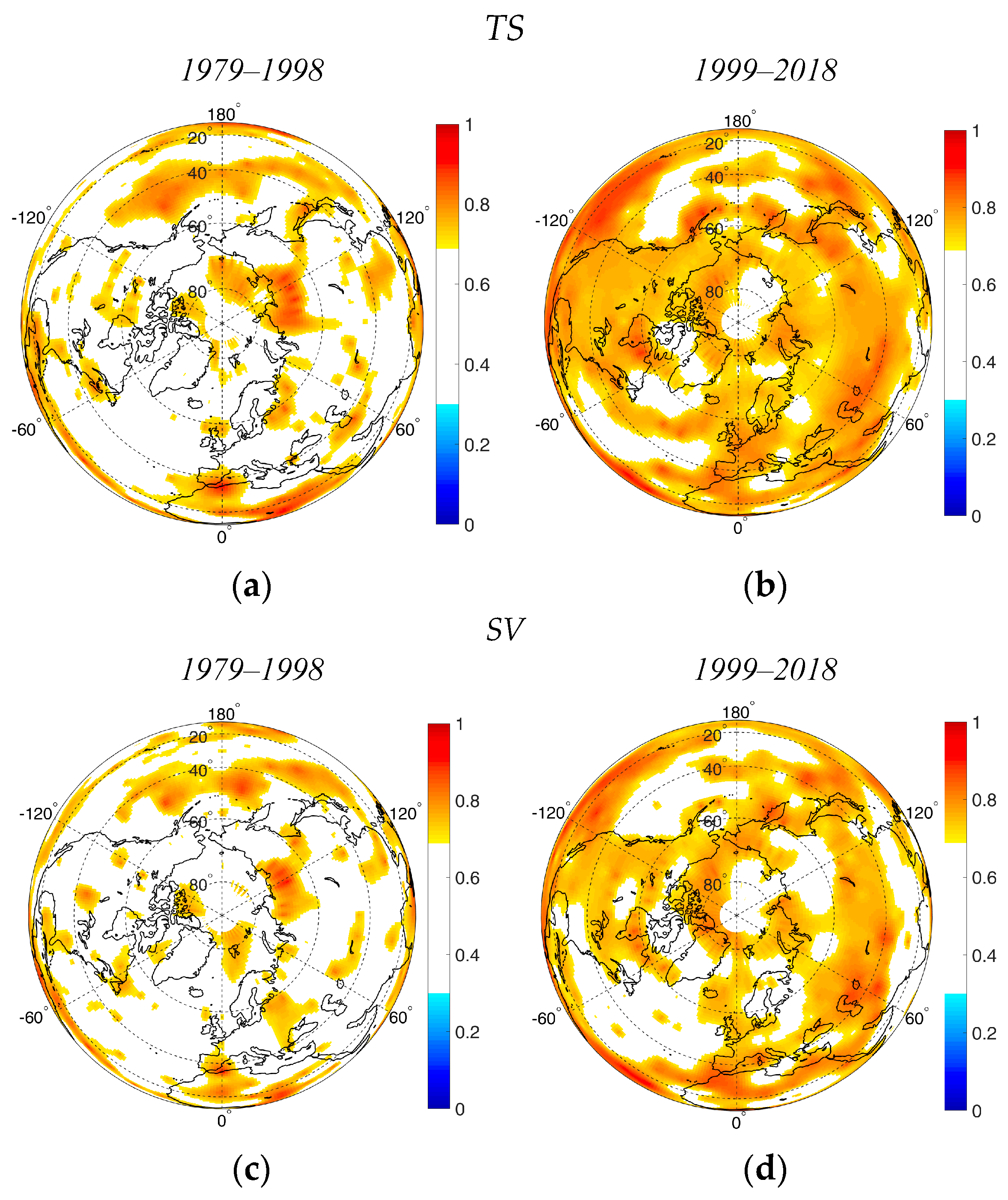
As can be observed in Table 2, at 850 hPa, the largest areas (among all parameters) with H > 0.72 in the Northern Hemisphere are typical for ω′ for both TS and SV scales for all seasons. Moreover, at the beginning of the 21st century, compared to the end of the 21st century, these areas increased. The maximum rise is observed in summer for TS from 16.6% to 69.0% and is probably caused by the increase in the southeastern part of the Pacific Ocean (Table 2, Figure 6). In winter, it was revealed that at the beginning of the 21st century, the areas of regions with H > 0.72 in general increase, especially in the eastern part of the Russian Arctic in the Arctic Ocean, in Eurasia, in the central part of North America and in the southeastern part of the Pacific Ocean.
The areas with anomalies of specific humidity also increase in summer, especially for TS (Table 2). However, a significant rise can also be observed in winter for SV. Regions with H > 0.72 (in winter and in summer) are mainly located over the following continents: in the northeastern part of Eurasia and North America, as well as in the tropical and the subtropical latitudes (Figure 7). At the same time, in summer, besides positive anomalies, negative anomalies are also observed, and they occupy significant areas (~30% at the beginning of the 21st century).
The same situation in the beginning of the 21st century (significant rise) for areas with H > 0.72 was also observed for u′ and v′ at TS and SV scales (Table 2).
The maximum increase for N (u′) is observed in summer for SV from 1.6% to 8%, and for N + (u′), it was 0% to 3.6% (Table 2). As for the spatial distribution, the maximum increase in the area with H > 0.72 at the beginning of the 21st century is observed in the low latitudes of the Pacific and Atlantic Oceans (Figure 8).
We suppose that the increase in meteorological anomalies observed in the low latitudes of the Pacific Ocean over recent decades could indicate an enhanced influence of El Niño events [41].
The specific feature in the t′ spatial distribution for TS and SV is the predominance of regions with H < 0.3 that occupy almost the entire area of the Northern Hemisphere: ~94% in winter at the beginning of the 21st century; ~80% in summer, both in the first and the second time interval. At that time, areas with H > 0.72 occupy no more than ~5% only in the summer season.
The regions with H > 0.72 for Φ′ were not revealed; therefore, Φ′ variability is not analyzed in this section.
It is worth noting that there are regions with H < 0.3 for some values. This indicates that it is difficult to forecast the tendency (i.e., antipersistent process). For example, for q′ anomalies in summer, vast regions with H < 0.3 dominated in the end of the 21st century in the spatial distribution (Figure 7). In winter, only a few isolated regions can be observed over the oceans at the end of the 21st century in the south (Figure 7).
The number of fractals for TS and SV scales and for all meteorological parameters’ anomalies with H > 0.72 varies in the range from 4.4 to 5.3, which means that the time series of anomalies have a long-term memory of 4 years. This can indicate that there is a power-law nature in the temporal variability [37]. At the same time, SV anomalies are more trend-resistant, relative to TS anomalies. The derived values of long-term memory are consistent with the effective correlation length calculated by the autocorrelation function module [42].
Thus, the application of fractal analysis has enabled the identification of regions in the Northern Hemisphere where power functions with the corresponding value of long-term memory can be used to describe the temporal variability of anomalies. It also helps in identifying regions where variability can be represented as an oscillatory process.

4. Discussion

In this study, we conducted an analysis of the spatial and temporal variability of climatic parameter anomalies, including those at the synoptic scale compared to the initial time series, in the Northern Hemisphere over the period from 1979 to 2018.
We distinguished three types of PDFs for the initial time series (selected for specified latitudinal zones). According to the classification in [16], for the North American region, several PDF types with different asymmetries can be defined for just one variable, such as temperature. Each meteorological variable has its individual PDF shape, which can shift under the mean state of the climate [19,20,21].
In our study, we found that the threshold values of anomalies derived from the initial time series should be determined for each considered variable, depending on various factors such as region, season, and level in the troposphere. In contrast, for the synoptic scale, we identified uniform boundaries for non-Gaussian anomalies across all variables: aN = −2.5 and aP = 3. The proposed approach allows for the determination of intervals of extreme non-Gaussian anomalies from the empirical PDFs of the main meteorological variables. Then, taking into account the value of a, it facilitates the analysis of climatic variability. However, relying solely on the climatology of the first four moments (mean value, variance, asymmetry, kurtosis) will not yield accurate estimates of the intervals for extreme anomalies.
Based on our results, at the beginning of the 21st century, compared to the end of the 20th century, the number of ω′ and q′ anomalies generally increases for both TS and SV scales in the Northern Hemisphere, with the maximum changes observed in the high latitudes. However, the number of u′ anomalies decreases in these regions, while it increases in the low and mid-latitudes during winter and spring. Anomalies or extreme values of climatic variables (u′, ω′ and q′) often occur in spatially coherent regions, suggesting a significant role of large-scale climatological forcing [12,43], particularly in the dynamics of atmospheric circulation (centers of atmospheric action, meridional circulation cells, cyclones and anticyclones, storm tracks, blockings, and others).
In particular, these tendencies may be associated with changes in the characteristics of regions with strong baroclinity (storm tracks) located near ~40° N, predominantly over the Pacific and Atlantic Oceans. According to [44,45,46], there is an observed increase in the intensity of storm tracks and their northward shift in the Northern Hemisphere. However, in some cases in the Atlantic region, such as during sudden stratospheric warming events or the eastern phase of the quasi-biennial oscillation, there can be a tendency for these tracks to weaken and shift towards lower latitudes [47,48]. The differences in weather conditions and the spread of synoptic-scale waves from the subtropics of the Pacific Ocean to the Atlantic region [46] contribute to these variations. Additionally, the variability of meridional circulation cells has significantly influenced the shift of storm track areas in recent decades. In the low latitudes, the Hadley cell [49,50,51,52] has expanded poleward over the past few decades, leading to the intensification of arid zones and baroclinic eddies. In the extratropics, both the Ferrell cell and the Hadley cell have shifted northward, while the polar cell has weakened [53,54]. This shift has resulted in the formation of anomalously warm conditions in the high latitudes of Eurasia and anomalously cold conditions in Greenland, the northeastern part of Africa, and the southwestern part of China [55]. According to our study’s results, these regions are characterized by the maximum number of specific humidity anomalies and the horizontal and vertical components of wind speed (as shown in Figure 4 and Figure 5). This suggests that the changes in anomalies, as well as their PDFs, may be associated with advective and convective transfer of heat and moisture [9,31].
Areas with the maximum number of ω′ anomalies are formed directly near the atmospheric centers of action, such as the Icelandic and Aleutian Lows, as well as the Azores and Hawaiian Highs. These areas are primarily located in the middle latitudes of the Pacific and Atlantic Oceans, near the Gulf Stream and the Kuroshio Currents, and in subpolar gyres. It is likely that synoptic-scale processes cause these anomalies in the Pacific Ocean across all seasons. In the Atlantic Ocean, however, these anomalies are observed only in summer, while in winter, the formation of ω′ is influenced by processes from other time scales.
The revealed distributions of q′, t′, v′, and u′ are predominantly located in continental regions, and their variability could be caused by atmospheric blocking of zonal transport in the troposphere at northern latitudes, which is associated with wave processes [56,57,58,59]. For example, in the winter season, their maximum number is concentrated in the north of the Far East, the northern part of North America, and the Siberian region near the Siberian High [32,60]. When comparing spatial distribution maps of skewness with those in [18], areas with extreme values (more than 3σ for long tails) were not observed. We suppose that this result is due to the different approaches used in anomaly calculation.
The processes of atmospheric circulation considered above contribute to the occurrence of extreme values of climatic parameters (non-Gaussian anomalies), as identified in our study. Therefore, standard Gaussian statistics methods (mean, variance) do not provide complete information about the stability of time series tendencies. The application of R/S analysis and multifractal analysis in our study to time series of extreme values in regions of the Northern Hemisphere has enabled us to determine the nature of the system’s behavior stability (trend-resistant or anti-persistent time series of anomalies). These methods also help identify regions where temporal variability can be described by a power-law dependence with the corresponding value of long-term memory, as well as regions where variability can be represented as an oscillatory process. The results obtained against the backdrop of a rapidly changing climate will be useful for refining and testing climatic models that also address prognostic problems.
According to [1], the risk of occurrence, as well as the duration and intensity of extreme events, is expected to increase in the future. Applying the aforementioned methods to the study of extreme values of climatic variables is highly significant for predicting their future trends. The originality of our work lies in the analysis of interval threshold values (with an accuracy of 0.25σ) for the PDF of non-Gaussian extreme anomalies. This approach is justified when a significant deviation from the Gaussian distribution is observed. Furthermore, it has enabled us not only to identify synoptic-scale processes amidst general disturbances but also to establish typical threshold values for the range of extreme values: |a| = 2.5–3. The difficulties associated with this approach include determining the frequency of rare extreme events and using short time intervals (such as 20 and 40 years). The latter limitation only permits a qualitative assessment of the interannual variability of parameters. To obtain statistically valid conclusions (with an alpha level of 0.05), the time series must contain several hundred values or more.
According to the results obtained, it is important to consider the role of the ocean in forming anomalies of climatic parameters, not only over oceanic areas but also on the continents of the Northern Hemisphere. In this context, atmospheric circulation becomes a significant climate-forming factor. This is because air masses, while passing over areas of intense heat and moisture exchange, undergo transformation and transport heat and moisture to the continents, thus affecting climate variability [31].
Thus, the novelty of our study is in the classification of PDF types and the determination of intervals for non-Gaussian extreme anomalies of the main six meteorological variables (air temperature, specific humidity, zonal, meridional and vertical wind speed, geopotential), while in many studies, the analysis for only one or two meteorological parameters is presented [12,13,16,17,18]. Moreover, it is also crucial that we identify the long-term nonlinear variability of anomalies based not only on their initial time series, but also on a sample with a synoptic time scale.
It should be noted that in this analysis, we do not consider high-frequency variability (with periods of less than one day) or low-frequency variability, which characterizes blocking processes (with periods ranging from 9 to 30 days) and interseasonal variability (such as the Madden–Julian Oscillation, with a period from 30 to 60 days). In the future, incorporating fluctuations at these scales could provide more reliable estimates of the relationship between anomalies and atmospheric circulation processes. It may also help in understanding the role of these processes in the occurrence of anomalies at both global and regional scales.

5. Conclusions

We analyzed the spatial and temporal variability in the number of non-Gaussian extreme anomalies of climatic parameters, covering both the initial time series and the synoptic scale in the Northern Hemisphere for the period 1979–2018. Three types of empirical distribution densities have been identified for the initial time series: (1) Type A—a distribution close to Gaussian, including anomalies in air temperature, zonal and meridional wind speed components in the boundary layer, and zonal wind speed and geopotential in the middle troposphere; (2) Type B—a distribution with positive/negative skewness, as seen in the anomalies of specific humidity and geopotential; (3) Type C—a distribution with significant kurtosis and notable exceedances of PDF values over the Gaussian in both negative and positive value areas, characteristic of anomalies in the vertical wind speed component. From this, we conclude that each type can characterize the processes of advective and convective heat transfer. Furthermore, we observed changes in the PDF types for these anomalies after filtering the initial time series.
It has been established that at the beginning of the 21st century, compared to the end of the 20th century, there is a general increase in the number of vertical velocity and specific humidity anomalies in the Northern Hemisphere for both synoptic and initial time series, with the most significant changes observed in the high latitudes. However, the number of zonal wind speed anomalies decreases in these regions, while it increases in the low and mid-latitudes during winter and spring. The regions with the highest number of climatic parameter anomalies are primarily located over the following continents: in winter, these include the northern part of the Far East and North America, as well as the Siberian region; in summer, they are found in the low latitudes. An exception is noted for vertical wind speed anomalies; they are mainly located over the oceans, specifically in the middle latitudes of the Pacific and Atlantic Oceans near the Kuroshio and Gulf Stream currents, and in subpolar gyres.
The application of R/S analysis and multifractal analysis in our study has made it possible to establish that, at the beginning of the 21st century compared to the end of the 20th century, areas with a Hurst parameter greater than 0.72 have increased, with the maximum rise observed in summer. The identified trends are expected to persist in the aforementioned regions and in the ocean areas of the Russian Arctic. Concurrently, there is a decrease in regions characterized by anti-persistent processes. It was also found that the time series of non-Gaussian anomalies (both at initial and synoptic scales) exhibit a long-term memory of approximately 4 years. Furthermore, anomalies at the synoptic scale are more predictable compared to those from the initial series.
Thus, we present the classification of non-Gaussian extreme anomalies based on their empirical distribution densities; reveal the specific features of spatial and temporal variability of each type and estimate the persistence of obtained tendencies in anomalies.
The results obtained, particularly against the backdrop of rapid climate change, will be useful for refining and testing numerical models that address prognostic issues in climatology.

Author Contributions

Conceptualization, S.L., E.M. and E.K.; methodology, S.L., E.M. and E.K.; software, S.L. and E.M.; formal analysis, S.L., E.K. and E.M.; investigation, E.K. and E.M.; resources, and data curation, E.M. and S.L.; writing—original draft preparation, E.K. and E.M.; writing—review and editing, S.L., E.K., E.M. and I.S.; visualization, S.L. and E.M.; supervision and project administration, S.L. and I.S.; funding acquisition, I.S. All authors have read and agreed to the published version of the manuscript.

Funding

This research was funded by the Russian Science Foundation (RSF), project # 21-71-10052, https://rscf.ru/en/project/21-71-10052 (accessed on 1 January 2024). S.L. and E.M. were supported by the Ministry of Science and Higher Education of the Russian Federation, project # 121031300154-1.

Institutional Review Board Statement

Not applicable.

Informed Consent Statement

Not applicable.

Data Availability Statement

The ERA-Interim reanalysis data were downloaded from https://www.ecmwf.int/en/forecasts/dataset/ecmwf-reanalysis-interim (accessed on 1 January 2024) [36].

Conflicts of Interest

The authors declare no conflicts of interest.

Abbreviations

PDFProbability distribution function
TSInitial time series
SVTime series of synoptic variability
tAir temperature anomaly
qSpecific air humidity anomaly
uZonal wind speed component anomaly
vMeridional wind speed component anomaly
ωVertical wind speed component anomaly
ΦGeopotential anomaly
N Number of negative anomalies
N + Number of positive anomalies
NNumber of anomalies ( N , N + , or N + N + )
aNThe area of negative anomalies
aPThe area of positive anomalies
W G Gaussian distribution
W E Non-Gaussian (empirical) distribution
HHurst parameter
LLow latitudes
MMiddle latitudes
HHigh latitudes

References

  1. IPCC. 2021: Climate Change 2021: The Physical Science Basis Contribution of Working Group I to the Sixth Assessment Report of the Intergovernmental Panel on Climate Change; Masson-Delmotte, V., Zhai, P., Pirani, A., Connors, S.L., Péan, C., Berger, S., Caud, N., Chen, Y., Goldfarb, L., Gomis, M.I., et al., Eds.; Cambridge University Press: Cambridge, UK; New York, NY, USA, 2021; 2391p. [Google Scholar] [CrossRef]
  2. Hansen, J.; Sato, M.; Ruedy, R. Perception of climate change. Proc. Natl. Acad. Sci. USA 2012, 109, E2415–E2423. [Google Scholar] [CrossRef] [PubMed]
  3. Castillo, F.; Wehner, M.; Stone, D.A. Extreme Events and Climate Change: A Multidisciplinary Approach; John Wiley & Sons: Hoboken, NJ, USA, 2021; p. 226. [Google Scholar]
  4. Goyal, M.K.; Gupta, A.K.; Gupta, A. Hydro-Meteorological Extremes and Disasters; Springer Nature: Singapore, 2022; p. 328. [Google Scholar]
  5. Kirtman, B.; Power, S.B.; Adedoyin, A.J.; Boer, G.J.; Bojariu, R.; Camilloni, I.; Doblas-Reyes, F.J.; Fiore, A.M.; Kimoto, M.; Meehl, G.A.; et al. Near-term climate change: Projections and predictability. In Climate Change 2013: The Physical Science Basis; Stocker, T.F., Qin, D., Plattner, G.-K., Tignor, M., Allen, S.K., Boschung, J., Nauels, A., Xia, Y., Bex, V., Midgley, P.M., Eds.; Cambridge University Press: Cambridge, UK, 2013; pp. 953–1028. [Google Scholar]
  6. Bardin, M.Y.; Platova, T.V. Long-period variations in extreme temperature statistics in Russia as linked to the changes in large-scale atmospheric circulation and global warming. Russ. Meteorol. Hydrol. 2019, 44, 791–801. [Google Scholar] [CrossRef]
  7. Kharyutkina, E.V.; Loginov, S.V.; Moraru, E.I.; Pustovalov, K.N.; Martynova, Y.V. Dynamics of extreme climatic characteristics and trends of dangerous meteorological phenomena over the Territory of Western Siberia. Atmos. Ocean. Opt. 2022, 35, 394–401. [Google Scholar] [CrossRef]
  8. Shumakov, I.A. Third Roshydromet Assessment Report on Climate Change and Its Consequences in Russian Federation; Roshydromet, Naukoemkie Tekhnologii: Saint Petersburg, Russia, 2022; 124p. [Google Scholar]
  9. Quan, H.; Zhang, B.; Bourguet, S.; Linz, M.; Chen, G. How Do Different Processes Shape Temperature Probability Distributions? A Percentile-Averaged Temperature Tendency Decomposition. J. Clim. 2023, 36, 5179–5196. [Google Scholar] [CrossRef]
  10. Schneider, T.; Bischoff, T.; Płotka, H. Physics of changes in synoptic midlatitude temperature variability. J. Clim. 2015, 28, 2312–2331. [Google Scholar] [CrossRef]
  11. Kononova, N.K. Types of the global atmospheric circulation: Monitoring and retrospective assessment results of 1899–2017 Fundament. Prikl. Klimatol. 2018, 3, 108–123. [Google Scholar] [CrossRef]
  12. Garfinkel, C.I.; Harnik, N. The non-Gaussian and spatial asymmetry of temperature extremes relative to the storm track: The role of horizontal advection. J. Clim. 2017, 30, 445–464. [Google Scholar] [CrossRef]
  13. Hassanzadeh, P.; Kuang, Z. Blocking variability: Arctic Amplification versus Arctic Oscillation. Geophys. Res. Lett. 2015, 42, 8586–8595. [Google Scholar] [CrossRef]
  14. Semenov, V.A.; Mokhov, I.I.; Latif, M. Influence of the ocean surface temperature and sea ice concentration on regional climate changes in Eurasia in recent decades. Izv. Atmos. Ocean. 2012, 48, 355–372. [Google Scholar] [CrossRef]
  15. Semenov, V.A. Link between anomalously cold winters in Russia and sea-ice decline in the Barents Sea. Izv. Atmos. Ocean. Phys. 2016, 52, 225–233. [Google Scholar] [CrossRef]
  16. Loikith, P.C.; Lintner, B.R.; Kim, J.; Lee, H.; Neelin, J.D.; Waliser, D.E. Classifying reanalysis surface temperature probability density functions (PDFs) over North America with cluster analysis. Geophys. Res. Lett. 2013, 40, 3710–3714. [Google Scholar] [CrossRef]
  17. Tamarin-Brodsky, T.; Hodges, K.; Hoskins, B.J.; Shepherd, T.G. A Dynamical Perspective on atmospheric temperature variability and its response to climate change. J. Clim. 2019, 32, 1707–1724. [Google Scholar] [CrossRef]
  18. Perron, M.; Sura, P. Climatology of Non-Gaussian Atmospheric Statistics. J. Clim. 2013, 26, 1063–1083. [Google Scholar] [CrossRef]
  19. Easterling, D.R.; Meehl, G.A.; Parmesan, C.; Changnon, S.A.; Karl, T.R.; Mearns, L.O. Climate extremes: Observations, modeling, and impacts. Science 2000, 289, 2068–2074. [Google Scholar] [CrossRef] [PubMed]
  20. Brönnimann, S.; Luterbacher, J.; Ewen, T.; Diaz, H.F.; Stolarski, R.S.; Neu, U. Climate Variability and Extremes during the Past 100 Years, 1st ed.; Springer: Berlin/Heidelberg, Germany, 2008; 364p. [Google Scholar]
  21. Houghton, J. Global Warming: The Complete Briefing, 4th ed.; Cambridge University Press: Cambridge, UK, 2009; 438p. [Google Scholar]
  22. Ruff, T.W.; Neelin, J.D. Long tails in regional surface temperature probability distributions with implications for extremes under global warming. Geophys. Res. Lett. 2012, 39, L04704. [Google Scholar] [CrossRef]
  23. Loikith, P.C.; Neelin, J.D. Short-tailed temperature distributions over North America and implications for future changes in extremes. Geophys. Res. Lett. 2015, 42, 8577–8585. [Google Scholar] [CrossRef]
  24. Loikith, P.C.; Broccoli, A.J. Characteristics of Observed Atmospheric Circulation Patterns Associated with Temperature Extremes over North America. J. Clim. 2012, 25, 7266–7281. [Google Scholar] [CrossRef]
  25. Sardeshmukh, P.D.; Compo, G.P.; Penland, C. Need for caution in interpreting extreme weather statistics. J. Clim. 2016, 28, 9166–9187. [Google Scholar] [CrossRef]
  26. Blackmon, M.L.; Wallace, J.M.; Lau, N.-C.; Mullen, S.L. An observational study of the Northern Hemi-sphere wintertime circulation. J. Atmos. Sci. 1977, 34, 1040–1053. [Google Scholar] [CrossRef]
  27. Petoukhov, V.; Eliseev, A.V.; Klein, R.; Oesterle, H. On statistics of the free-troposphere synoptic component: An evaluation of skewnesses and mixed third-order moments contribution to the synoptic-scale dynamics and fluxes of heat and humidity. Tellus 2008, 60 Pt A, 11–31. [Google Scholar] [CrossRef]
  28. Loginov, S.V.; Eliseev, A.V.; Mokhov, I.I. Impact of non-Gaussian statistics of atmospheric variables on extreme intramonth anomalies. Izv. Atmos. Ocean. Phys. 2017, 53, 269–278. [Google Scholar] [CrossRef]
  29. Linz, M.; Chen, G.; Hu, Z. Large-scale atmospheric control on non-Gaussian tails of midlatitude temperature distributions. Geophys. Res. Lett. 2018, 45, 9141–9149. [Google Scholar] [CrossRef]
  30. Loikith, P.C.; Neelin, J.D.; Meyerson, J.; Hunter, J.S. Short warm-side temperature distribution tails drive hotspots of warm temperature extreme increases under near-future warming. J. Clim. 2018, 31, 9469–9487. [Google Scholar] [CrossRef]
  31. Moraru, E.I.; Loginov, S.V.; Kharyutkina, E.V. Features of the spatiotemporal variability of the advective heat transfer in the troposphere over the Pacific and Atlantic oceans in the Northern Hemisphere for 1979–2018. Izv. Atmos. Ocean. Phys. 2021, 57, 693–700. [Google Scholar] [CrossRef]
  32. Mokhov, I.I.; Chernokulsky, A.V.; Osipov, A.M. Atmospheric centers of action in the Northern and Southern hemispheres: Features and variability. Russ. Meteorol. Hydrol. 2020, 45, 749–761. [Google Scholar] [CrossRef]
  33. Loginov, S.V.; Kharyutkina, E.V. Application of fractal and wavelet analysis to the assessment of climate changes in West Siberia over winter season. Izv. Vuzov Fizika 2016, 59, 139–143. [Google Scholar] [CrossRef]
  34. Ippolitov, I.I.; Kabanov, M.V.; Loginov, S.V. Spatiotemporal scales of warming observed in Siberia. Dokl. Earth Sci. 2007, 413, 248–251. [Google Scholar] [CrossRef]
  35. Huang, N.E.; Shen, S.P. Hilbert-Huang Transform and Its Application; World Scientific: Singapore, 2005; 311p. [Google Scholar]
  36. Dee, D.P.; Uppala, S.M.; Simmons, A.J.; Berrisford, P.; Poli, P.; Kobayashi, S.; Andrae, U.; Balmaseda, M.A.; Balsamo, G. The ERA-Interim reanalysis: Configuration and performance of the data assimilation system. Q. J. R. Meteorol. Soc. 2011, 137, 553–597. [Google Scholar] [CrossRef]
  37. Feder, E. Fractals; Springer Science and Business Media: Berlin/Heidelberg, Germany, 2013; 284p. [Google Scholar]
  38. Weron, R. Estimating long-range dependence: Finite sample properties and confidence intervals. Phys. A Stat. Mech. Appl. 2002, 312, 285–299. [Google Scholar] [CrossRef]
  39. Lyubushin, A.A. Low-Frequency Seismic Noise Properties in the Japanese Islands. Entropy 2013, 23, 474. [Google Scholar] [CrossRef]
  40. Ventura, V.; Paciorek, C.J.; Risbey, J.S. Controlling the proportion of falsely rejected hypotheses when conducting multiple tests with climatological data. J. Clim. 2004, 17, 4343–4356. [Google Scholar] [CrossRef]
  41. Osipov, A.M.; Gushchina, D.Y. El-Nino 2015–2016: Evolyuciya, mekhanizmy, soputstvuyushchie udalennye anomalii. Fund. Prikl. Klim. 2018, 3, 54–81. [Google Scholar]
  42. Franceschetti, G.; Riccio, D. Scattering, Natural Surfaces, and Fractals; Elsevier: Amsterdam, The Netherlands, 2007; 304p. [Google Scholar] [CrossRef]
  43. Stefanova, L.; Sura, P.; Griffin, M. Quantifying the non-Gaussianity of wintertime daily maximum and minimum temperatures in the Southeast. J. Clim. 2016, 26, 838–850. [Google Scholar] [CrossRef]
  44. Eichler, T.P.; Gaggini, N.; Pan, Z. Impacts of global warming on Northern Hemisphere winter storm tracks in the CMIP5 model suite. Geophys. Res. Lett. 2013, 118, 3919–3932. [Google Scholar] [CrossRef]
  45. Tamarin, T.; Kaspi, Y. The poleward shift of storm tracks under global warming: A Lagrangian perspective. Geophys. Res. Lett. 2017, 20, 10666–10674. [Google Scholar] [CrossRef]
  46. Martynova, Y.V.; Vargin, P.N.; Volodin, E.M. Variation of Northern Hemispheric wintertime storm tracks under future climate change in INM-CM5 simulations. Izv. Atmos. Ocean. 2022, 58, 208–218. [Google Scholar] [CrossRef]
  47. Wang, J.; Kim, H.-M.; Chang, E. Interannual Modulation of Northern Hemisphere Winter Storm Tracks by the QBO. Geophys. Res. Lett. 2018, 45, 2786–2794. [Google Scholar] [CrossRef]
  48. Afargan-Gerstman, H.; Domeisen, D. Pacific Modulation of the North Atlantic Storm Track Response to Sudden Stratospheric Warming Events. Geophys. Res. Lett. 2020, 47, e2019GL085007. [Google Scholar] [CrossRef]
  49. Mitas, C.M.; Clement, A. Recent behavior of the Hadley cell and tropical thermodynamics in climate models and reanalyses. Geophys. Res. Lett. 2006, 33, L01810. [Google Scholar] [CrossRef]
  50. Fu, Q.; Johanson, C.M.; Wallace, J.M.; Reichler, T. Enhanced mid-latitude tropospheric warming in satellite measurements. Science 2006, 312, 1179. [Google Scholar] [CrossRef] [PubMed]
  51. Lu, J.; Vecchi, G.A.; Reichler, T. Expansion of the Hadley cell under global warming. Geophys. Res. Lett. 2007, 34, L06805. [Google Scholar] [CrossRef]
  52. Mbengue, C.; Schneider, T. Storm-track shifts under climate change: Toward a mechanistic understanding using baroclinic mean available potential energy. J. Atmos. Sci. 2017, 74, 93–110. [Google Scholar] [CrossRef]
  53. Dima, I.M.; Wallace, J.M. On the seasonatity of the Hadley cell. J. Atmos. Sci. 2003, 60, 1522–1527. [Google Scholar] [CrossRef]
  54. Loginov, S.V.; Moraru, E.I.; Kharyutkina, S.V. Relationship of tropospheric circulation cells with the variability of meridional heat flows over Siberia. Opt. Atmos. Okeana 2016, 29, 640–646. [Google Scholar] [CrossRef]
  55. Doos, K.; Nilsson, J. Analysis of the meridional energy transport by atmospheric overturning circulations. J. Atmos. Sci. 2011, 68, 1806–1819. [Google Scholar] [CrossRef]
  56. Thorncroft, C.D.; Hoskins, B.J.; McIntyre, M.E. Two Paradigms of Baroclinic-Wave Life-Cycle Behaviour. Q. J. R. Meteorol. Soc. 1993, 119, 17–55. [Google Scholar] [CrossRef]
  57. Hoskins, B.J.; McIntyre, M.E.; Robertson, A.W. On the Use and Significance of Isentropic Potential Vorticity Maps. Q. J. R. Meteorol. Soc. 2007, 111, 877–946. [Google Scholar] [CrossRef]
  58. Iwao, K.; Takahashi, M.A. Precipitation seesaw mode between Northeast Asia and Siberia in summer caused by Rossby Waves over the Eurasian continent. J. Clim. 2008, 21, 2401–2419. [Google Scholar] [CrossRef]
  59. Schubert, S.D.; Wang, H.; Koster, R.D.; Suarez, M.J.; Groisman, P.Y. Northern Eurasian heat waves and droughts. J. Clim. 2014, 27, 3169–3207. [Google Scholar] [CrossRef]
  60. Chernokulsky, A.V.; Bulygina, O.N.; Mokhov, I.I. Recent variations of cloudiness over Russia from surface daytime observations. Environ. Res. Lett. 2011, 6, 035202. [Google Scholar] [CrossRef]
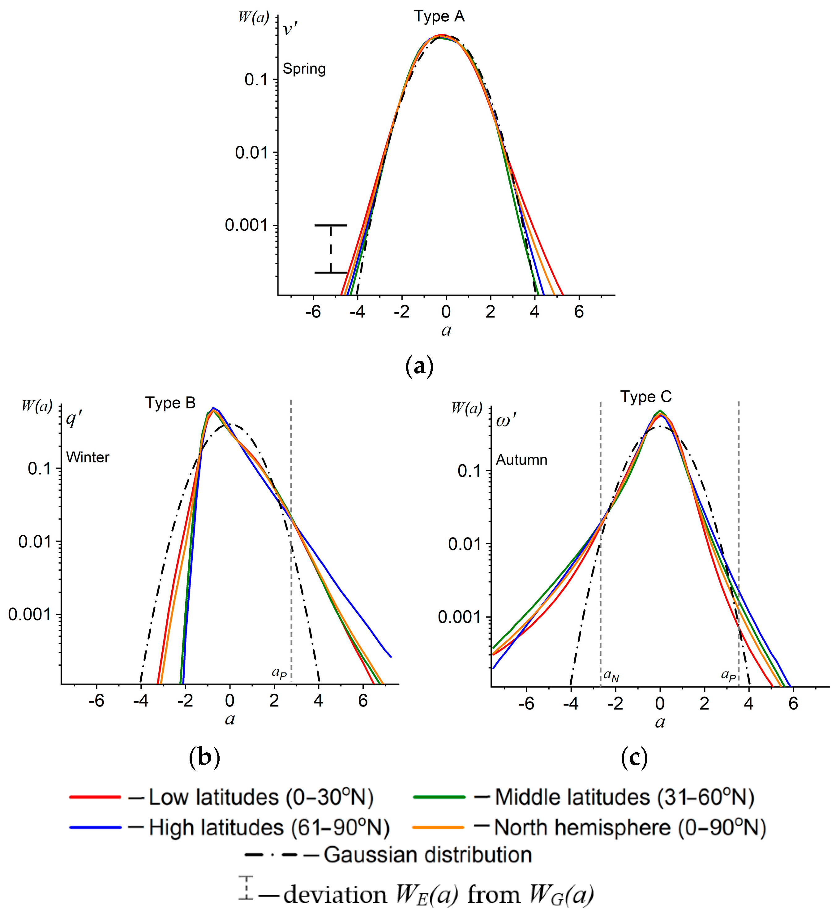
Figure 1. The PDF types of seasonal climatic parameter anomalies (TS) over the period of 1979–2018 for the latitudinal zones in the Northern Hemisphere at 500 hPa: v′ (a), q′ (b), ω′ (c).
Climate 12 00008 g001
Figure 2. Spatiotemporal variability of aN and aP for anomalies of climatic parameters in latitudinal zones of the Northern Hemisphere (L—low latitudes, M—middle latitudes, H—high latitudes) over 1979–2018: TS (a); SV (b).
Climate 12 00008 g002
Figure 3. Anomaly number of climatic parameters in the Northern Hemisphere (L—low latitudes, M—middle latitudes, H—high latitudes) over the period 1979–2018: left panel—TS, right panel—SV; I—winter, II—spring, III—summer, IV—autumn.
Climate 12 00008 g003
Figure 4. Spatial variability of N for TS at 850 hPa in winter (a,c) and in summer (b,d) over the period of 1979–2018. Red dash line— N + , blue dash line— N (specified by 0.95 quantile).
Climate 12 00008 g004
Figure 5. The same as in Figure 4 for SV in winter (a,c) and in summer (b,d).
Climate 12 00008 g005
Figure 6. Spatial distribution of the H parameter for N (ω′) for TS (a,b) and SV (c,d) at 850 hPa in summer.
Climate 12 00008 g006
Figure 7. Spatial distribution of the H parameter for N(q′) for TS at 850 hPa in summer.
Climate 12 00008 g007
Figure 8. Spatial distribution of the H parameter for N(u′) for SV at 850 hPa in summer.
Climate 12 00008 g008
Table 1. The ratio of the PDF types (in %) of TS anomalies and SV anomalies over the period 1979–2018. The line “Anomalies” presents only the anomalies with a percentage of 20% and higher from the total anomaly number for a certain type. The order in which anomalies are listed corresponds to the size of their part.
HeightTS, %SV, %
Type AType BType CType AType BType C
850 hPa26532133463
Anomaliest′, u′, vq′, Φω′, vv′, ΦΦ′, uω′, q′, t
500 hPa19483363757
Anomaliesu′, Φq′, Φ′, tω′, vv′, uΦ′, uω′, q
Table 2. Part of areas with H > 0.72 (in %) from the total area of the North Hemisphere for climatic parameter anomalies for TS and SV at 850 hPa: I—1979–1998, II—1999–2018.
SeasonWinterSummer
Anomaly SignNN+NN+
PeriodIIIIIIIIIIII
q
TS0014.713.62.94.30.31.7
SV11.118.215.725.610.213.611.111.6
t
TS00000000
SV00.10.300.1001.4
u
TS0.32.91.52.50.93.10.51.3
SV00.500.61.6803.6
v
TS0.41.04.813.90.61.713.119.6
SV00.200.20.42.10.54.3
ω
TS27.646.018.154.023.963.216.669.0
SV25.340.733.147.820.849.519.250.3
Disclaimer/Publisher’s Note: The statements, opinions and data contained in all publications are solely those of the individual author(s) and contributor(s) and not of MDPI and/or the editor(s). MDPI and/or the editor(s) disclaim responsibility for any injury to people or property resulting from any ideas, methods, instructions or products referred to in the content.