Abstract
The validated influence of urban biophysical structure on environmental processes within urban areas has heightened the emphasis on studies examining morphological patterns to determine precise locations and underlying causes of urban climate conditions. The present study aims to characterise morphological patterns describing the distribution of Land Surface Temperature (LST) based on a prior classification of biophysical variables, including urban density (building intensity and average height), surface characteristics, shortwave solar radiation (broadband albedo), and seasonal variations in vegetation cover (high, medium, and low levels), retrieved from multisource datasets. To describe the distribution of LST, the variables were calculated, classified, and subsequently, analysed individually and collectively concerning winter and summer LST values applied in an urban neighbourhood in Madrid, Spain. The results from the analytical approaches (observation, correlations, and multiple regressions) were compared to define the morphological patterns. The selection of areas resulting from the morphological patterns with the most unfavourable LST values showed agreement of up to 89% in summer and up to 70% for winter, demonstrating the feasibility of the methods applied to identify priority areas for intervention by season. Notably, low and high vegetation levels emerged as pivotal biophysical characteristics influencing LST distribution compared to the other characteristics, emphasising the significance of integrating detailed seasonal vegetation variations in urban analyses.
1. Introduction
As global temperature changes continue to be documented, there is a growing interest in understanding the factors driving these temperature fluctuations [1]. Within this context, urban environments are increasingly recognised as contributors to temperature changes at both local and larger scales [2]. Consequently, there has been a surge in research endeavours and studies aiming to identify and assess the biophysical characteristics—encompassing built-up and natural elements—that influence air and surface temperatures. These factors collectively shape the urban microclimate [3] and have implications for the provision or loss of regulating ecosystem services, among other crucial considerations [4,5,6].
One prominent method used to examine factors that influence the urban microclimate is the quantitative classification known as Local Climate Zones (LCZs), developed by Stewart and Oke [7]. LCZs encompass biophysical characteristics, incorporating built elements, land cover, and population data within urban settings, all of which play a role in shaping the local climate. Additionally, numerous research efforts have delved into urban population growth and expansion, the emergence of urban heat islands (UHIs) affecting both air and surface temperatures, and strategies involving vegetation cover and reflective surfaces to mitigate temperature rise and reduce heat stress. These studies underscored the significance of urban density and anthropogenic heat, which are often overlooked aspects of urban areas, as extensively reviewed by Chapman et al. [8].
The importance of urban studies that incorporate various biophysical characteristics influencing temperature changes in cities has been emphasised. However, conducting such research entails inherent complexities, encompassing challenges in data collection, processing, and costs, and accounting for spatio-temporal changes [9,10,11]. In response to these challenges, attempts have been aimed at establishing official datasets covering built-up areas [12]. Moreover, remote sensing tools have been employed to observe, categorise, and evaluate additional biophysical features such as water bodies and vegetation, seamlessly integrating them using Geographic Information Systems (GIS) software [13].
The availability of open-access databases, including cadastral data, has notably enhanced the efficiency of acquiring information of the built elements shaping urban environments [14]. Furthermore, the application of remote sensing, facilitating Earth observation, has seen significant technological advancements in spatial, spectral, radiometric, and temporal resolutions [15,16].
Remote sensing has also enabled the identification of vegetation cover, quantification of spatio-temporal changes in vegetation, assessment of ecosystem service provisioning, evaluation of socio-economic and vegetation dynamics, and measurement of Land Surface Temperature (LST) associated with temperature fluctuations, among various other applications [17]. Therefore, remote sensing emerges as a valuable alternative to ground-based assessments [18,19,20], playing a pivotal role in modern comprehensive urban studies that require observations of LST and vegetation dynamics [21].
From the inherent complexity in studying factors influencing temperature changes in urban settings, this study presents an approach centred on characterising morphological patterns. It evaluates biophysical variables and their associations with LST by retrieving these from multisource datasets, including open data and remote sensing tools, spanning two distinct periods—winter and summer—to account for spatio-temporal variations.
Three methods concerning statistical analysis and observational techniques were employed to characterise these patterns, drawing upon pre-existing classifications of biophysical variables detailed in a prior study [22] within the Canillas neighbourhood, in Madrid, Spain. The basis of this characterisation rests upon the distribution of LST across winter and summer seasons. This process enables the identification of areas warranting priority intervention, intricately linked to devising strategies aimed at improving hygrothermal conditions, counteracting the UHI effect, and addressing various other pertinent considerations.
2. Study Area
This study was conducted in Canillas, a mixed-use neighbourhood situated on the northeastern periphery of Madrid, Spain, covering an area of 2.52 km2 and inhabited by 39,708 residents [23]. Canillas has been an integral part of the city’s peripheral expansion since its integration in 1949 [24], and it has witnessed multiple urban transformations and population growth over the years [25].
The significance of carrying out the study in Canillas is underpinned by its peripheral location, the vibrant community life featuring sports facilities, a cycling track, green spaces, and the urban transformations it has undergone. The neighbourhood exhibits morphological diversity and falls within the Köppen–Geiger climate classification of Bsk, signifying hot summer Mediterranean conditions with scorching, arid summers, and mild, wet winters; the neighbourhood is thus more prone to effects such as UHI due to its climate fluctuations. These characteristics make it an ideal setting for investigating the spatio-temporal aspects of biophysical variables. The findings are anticipated to offer insights applicable to similar scenarios in southern European and Mediterranean cities also falling under the Bsk climate classification.
3. Methods and Data
This section provides an overview of the methods and data employed in this study, as depicted in Figure 1. Steps 1 to 3 outline the procedures for extracting biophysical characteristics and LST from the multisource datasets and their subsequent computations. Step 4 introduces the techniques for analysing the acquired data, incorporating the use of previously established classifications of biophysical characteristics. Step 5 illustrates the comparison of the outcomes derived from the conducted analyses aimed at characterising morphological patterns. The final step, Step 6, involves the identification of priority areas based on the characterised morphological patterns.
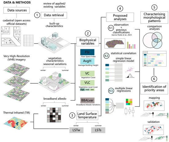
Figure 1.
Methods and data applied in the study [22].
3.1. Data Retrieval
This study utilised data from the Spanish cadastre databases, which included information about the built area at the subplot level and the number of storeys per building. We assessed biophysical variables identified in various studies pertaining to urban temperatures and climate [8,26,27,28,29]. Additionally, we incorporated very-high-resolution (VHR) Pléiades satellite imagery and Landsat 8 Operational Land Imager (OLI) imagery, which include Thermal Infrared (TIR) Band 10 (10.6–11.9 μm). Table 1 provides a comprehensive overview of the data sources used for extracting biophysical characteristics, along with the formulas employed for variable calculations in the study.
The calculated variables are associated with urban density (Floor Space Index (FSI) and Average Building Height (AvgH)), geophysical surface attributes, and their correlation with shortwave solar radiation flux (Broadband Albedo (BBA)). Moreover, vegetation cover was considered both in a general sense and across various levels (high, medium, and low) from a Normalised Difference Vegetation Index (NDVI) threshold. Elaborate methodologies for calculating urban density and vegetation variables are outlined in detail in García Pardo et al. [22].
In addition to these datasets, we employed ArcGIS Pro 2.9.0 software as the GIS for data processing. We organised the data for each characteristic into polygons by establishing an arbitrary grid based on the neighbourhood’s boundary. This approach yielded 219 polygons, each covering an equal surface area of 1 hectare. The selection of this grid and its dimensions were determined to be suitable for this study following a thorough review of the relevant literature [14,30,31,32]. The grid is widely acknowledged as the second most employed unit in urban studies and is comprehensively defined in the work of Liu et al. [33].
LST in this study was derived from ground pixel-level observations obtained from Landsat 8 imagery. We specifically used the TIR Band 10 and applied the NDVI method to calculate Land Surface Emissivity (LSE), as outlined in Sobrino, Jiménez-Muñoz, and Polini [34]. The computation of LST required several parameters acquired beforehand, including Top of Atmosphere spectral radiance (TOA), Brightness Temperature (BT), and Land Surface Emissivity (ε). The latter relies on NDVI and Proportion of Vegetation (PV) values. Regarding the calculation of Broadband Albedo, the method was adopted from Hidalgo-García [35].
Detailed descriptions of the biophysical characteristics considered in the study, information sources, calculation formulas for each biophysical variable, and concise variable explanations are provided in Table 1.

Table 1.
Data retrieval from multisource datasets and details.
Table 1.
Data retrieval from multisource datasets and details.
| Biophysical Type | Source and Data Type | Biophysical Variable | Formula | Description | |
|---|---|---|---|---|---|
Built-up | Spanish Cadastre shapefiles | Floor Space Index (FSI) | (1) | Building intensity from the total amount of enclosed area of all storeys within each building. | |
| Average Building Height (AvgH) | (2) | Mean building height. | |||
Vegetation | Pléiades Satellite_Airbus DS Geo SGSA VHR imagery | Vegetation Cover (VC) | (3) | Percentage of area occupied by vegetation on winter and/or summer dates over the study area. | |
| Vegetation Level Cover (VLC) high/medium/low | VLC (H/M/L) | (4) | The values for this characterisation were obtained from [36]:
| ||
Broadband Albedo | Unites States Geological Survey USGS Landsat 8 OLI + TIRS | Broadband Albedo (BBAlbedo) BBAlvar_w/s | Broadband Albedo [35] BBAlbedo = 0.356 * BBlue + 0.130 * BRed + 0.373 * BNIR + 0.085 * BSwir1+ 0.072 * BSwir2 − 0.0018 BBAlvar_w/s = The standard deviation of each polygon was extracted to obtain | (5) | Relationship between the surface upward flux and the downward flux of shortwave solar radiation over the ascending hemispherical space. |
Land Surface Temperature (LST) | Unites States Geological Survey USGS Landsat 8 OLI + TIRS | NDVI method [34]. | Emission of thermal radiance from a surface derived from solar radiation. | ||
| Top of Atmosphere | |||||
| (Lλ) | (6) | ||||
| Lλ | (7) | ||||
| Brightness Temperature | |||||
| (8) | |||||
| BT | (9) | ||||
| Proportion of Vegetation | |||||
| (10) | |||||
| Land Surface Emissivity | |||||
| (ε) | (11) | ||||
| Land Surface Temperature | |||||
| (LST) | (12) |
Note: is the total study area (1 ha); represents the building; represents the buildings’ footprints; F is the building’s total gross floor area; Bs represents the number of storeys; 3.00 m is a standard value assigned for all buildings above floor level. and are the spectral bands in the VHR Pléiades imagery; represents the polygons corresponding to the vegetation class from the supervised OBIA LCC; is the pixel characterised with a NDVI threshold vegetation level; and is the total number of pixels within the polygon (40,000); is the band-specific multiplicative rescaling factor retrieved from the imagery metadata; is the band-specific additive rescaling factor retrieved from the imagery metadata; corresponds to Band 10; and and are the band-specific thermal conversion constants from the imagery metadata.
3.2. Previous Classification of Biophysical Variables
The classifications of the biophysical variables, derived from a previous framework employed in this study found in García Pardo et al. [22], show four distinct built-up clusters further delineated based on the nuances of their general vegetation cover and across different vegetation levels. The methods employed for the classifications include statistical analyses and spatial autocorrelations assessments, using two distinct approaches: the k-means clustering method and categorisation based on standardised values.
The resulting classifications unveiled the potential to meticulously characterise the composition of urban environments and provide an overview of seasonal variations in vegetation cover at different levels. To enhance these classifications, variables associated with the variance in broadband albedo for each polygon, denoted BBAlvar, were introduced, and categorised based on the standard deviations to the overall set of values. BBAlvar categorisation follows the same approach applied to the vegetation variables in a previous study [22].
Figure 2 showcases the two previous classifications used in this study, demonstrating the incorporation of the proposed biophysical variables. These classifications highlight the importance of considering spatio-temporal scales in urban studies, revealing observable differences between seasons. This is particularly evident in the colour scale that delineates the vegetation categories assigned, and the standard deviation categories of BBAlvar to each polygon within the case study.
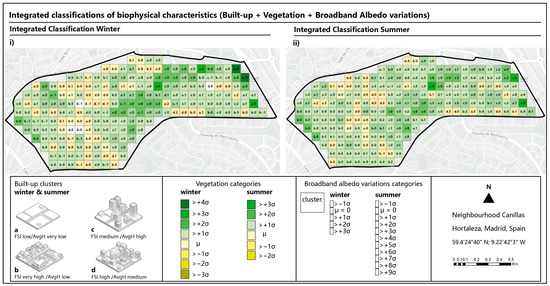
Figure 2.
Integrated classification of biophysical characteristics: (i) winter and (ii) summer.
3.3. Proposed Analyses to Identify Morphological Patterns
Three analysis methods are proposed: first, the parallel observation of classifications and LST groups; second, statistical correlation analyses for individual variables utilising a simple linear regression model (Y = a + b*X); and third, multiple regression analyses (Y = a + b1X1 + b2X2) considering LST as the dependent variable (Y) and biophysical factors as the dependent variables. It is important to note that the study’s focus is not on predicting LST but rather on comprehending the influence of each calculated variable on LST distribution.
To conduct the parallel observation of the previously made classifications (Section 3.2), the LST values obtained in each of the polygons needed to be categorised into groups based on the variation of ±1 K from the neighbourhood’s mean values. Subsequently, these values were mapped for both winter and summer. For LST in winter (LSTw), six groups were obtained ranging from −2 K to +3 K, with 0 representing the neighbourhood’s mean. For LST in summer (LSTs), eight groups were derived, ranging from −2 K to +5 K, indicating a more substantial temperature variation in summer compared to winter (refer to Figure 3).
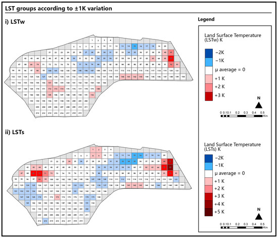
Figure 3.
Classification of LST values into groups according to ±1 K variation. (i) LSTw; (ii) LSTs.
The polygons belonging to each LST group were observed from their corresponding built-up cluster, vegetation categories, and the broadband albedo variation to identify coincidences in biophysical characteristics within each group.
Relationships between variables and LST were analysed using a simple linear regression model to ascertain significant relationships and their strength, and to obtain a regression equation to predict LST values from the adjusted model. This process involved evaluating the outcomes of each correlation (r), which indicates the strength and direction of the relationship of each variable in describing the LST variation. The p-value from the analysis of variance (ANOVA) was used to establish significant relationships between variables at a 95% confidence level, and the R-squared (R2) value indicated the percentage by which the variable explains LST based on the adjusted model. Observation of the scatterplots was also carried out to discern distribution patterns and fluctuations in variable values concerning LST’s. Moreover, exhibiting atypical residuals for each variable and their adjusted model were studied to detect anomalies and facilitate comparative assessments among them.
For the multiple variable regression analysis, the backward stepwise regression method was applied based on the literature reviewed to attain best-fit regression models by automating the tests with different groups of independent variables [35,36,37]. This method starts with a model that includes all independent variables until those that are statistically less significant (p-value > 0.05) are removed.
The descriptions derived from each analysis were compared, facilitating the discussions on the relationships among biophysical characteristics within the neighbourhood and the effectiveness of integrated classifications in depicting the distribution of LST. The conclusions drawn from these comparisons were crucial for identifying morphological patterns, which were subsequently mapped to detect priority intervention areas for both winter and summer seasons.
4. Results
4.1. Observation of Morphological Patterns from Classifications
In the results of the LSTw in +K groups compared to the mean (temperatures higher between 2.6 °C and 5.6 °C), we observe a predominance of polygons belonging to the built-up cluster “a”, vegetation categories below the mean (−1 to −3), and BBAlvar_w categories around the mean. For the polygons within the LSTw group corresponding to the mean 0 (temperatures between 0.6 °C and 2.5 °C), the “b” built-up cluster predominates, along with vegetation categories around and below the mean (0 to −3), and BBAlvar_w categories around the mean.
Regarding the LSTw −K groups compared to the mean (lower temperatures between 0.6 °C and −1.3 °C), we can distinguish polygons belonging to built-up cluster “c”, vegetation categories around and above the mean (0 to 4), and BBAlvar_w categories above the mean (indicating higher broadband albedo variation within the polygon).
Figure 4 exhibits bar charts with the count of polygons belonging to the classifications, separated by LSTw groups. This aids in comprehending the observation analysis following the presentation of distinct patterns. LSTw values below the mean (−K) appeared to be primarily affected by BBAlvar_w and vegetation cover above the neighbourhood’s mean. Conversely, polygons with lower overall vegetation cover exhibit higher LSTw values in groups above the mean (+K). Lastly, polygons within clusters with lower building intensity (a and b) demonstrate higher LSTw values, whereas those in clusters with higher building intensity and taller buildings showcase lower LSTw values.

Figure 4.
Observation analysis by LSTw groups and classified polygons.
For the analysis of LSTs in +K groups compared to the mean (higher temperatures between 33.6 °C and 38 °C), polygons belonging to built-up cluster “a”, vegetation categories around or below the mean (0 to −2), and BBAlvar_s categories around the mean are predominant. For the polygons corresponding to the mean LSTs (temperatures between 31.5 °C and 33.5 °C), the built-up cluster “b” is prevalent, with most vegetation categories around the mean and a similar distribution between categories −1 and +1. These polygons also exhibit BBAlvar_s categories around the mean.
In LSTs −K groups compared to the mean (lower temperatures between 29 °C and 31.6 °C), we observe polygons associated with built-up cluster “c”, vegetation categories around and above the mean, and BBAlvar_s categories around the mean.
Figure 5 presents bar charts delineating the count of polygons within a specific biophysical classification, separated by LSTs groups. This helps to understand the observation analysis, revealing distinct trends. LSTs values appear not to be influenced by the BBAlvar_s categories, seemingly having no significant influence on LSTs values. Polygons characterised by higher vegetation cover are primarily aligned with LSTs groups below the mean (−K), while the opposite is observed for polygons with lower vegetation cover situated in LSTs groups above the mean (+K). Finally, a noteworthy observation indicates that polygons within lower building intensity clusters exhibit higher LST values, whereas those within clusters featuring higher building intensity and taller buildings have lower LST values.

Figure 5.
Observation analysis by LSTs groups and classified polygons.
The results for both seasons exhibit several similarities particularly regarding vegetation cover and its influence on LST’s. Across both seasons, higher vegetation cover consistently leads to lower LST values. However, a notable distinction arises while the relationship is similar in both seasons; in the LSTs +K groups, moderate vegetation cover prevails, contrasting with low vegetation cover seen in LSTw +K. Another similarity pertains to urban density, as indicated by the built-up clusters associated with each polygon within the LST groups. It was identified that higher building intensity and height correspond with lower LST values.
4.2. Identification of Morphological Patterns from Statistical Correlation Analysis
The analysis of each variable with LSTw revealed the variables with significant relationships (p-value ≤0.05) considering [38], ranked by influence (R2) are VLCwL, AvgH, VLCwM, and VCw. Specifically, the results indicated that low-level vegetation cover has a more pronounced negative impact on LSTw compared to other variables, implying that an increase in low-level vegetation corresponds to a decrease in LSTw. Similarly, AvgH and VCw exhibit a negative relationship with LSTw. However, VLCwM portrays a contrasting relationship, suggesting that increased VLCwM is associated with higher values in LSTw. From these results, variables related to high-level vegetation and building intensity do not show a significant relationship with LSTw (see Table 2).

Table 2.
Statistical correlation from simple linear regression of each variable and LSTw_Winter.
In Figure 6, which features scatter plots, when values reach ≥1.0 (≥30%) for low-level vegetation cover, LSTw consistently shifts to <1.0 (falling between LSTw groups 0 K and −2 K) without exception. Furthermore, values <1.0 (<30%) in VLCwL display a wider dispersion among LSTw values, ranging from −0.9 to 1.1 (within LSTw groups 0 K or the mean). For the BBAlvar_w values >1.5, there is an upward trend in LSTw values. Conversely, variables AvgH and VCw, related to LSTw, do not demonstrate specific patterns. Finally for the general vegetation cover, a heterogeneous distribution is observed, but when values surpass −0.3 (>35%), there is a noticeable decrease in LSTw values.
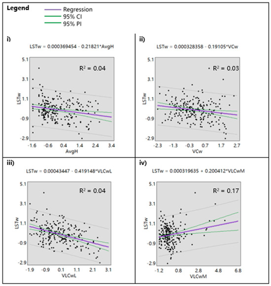
Figure 6.
Scatter plots from simple linear regression of variables with significant relationships with LSTw_Winter: (i) AvgH; (ii) VCw; (iii) VLCwL; and (iv) VLCwM.
In the observation of unusual residuals in variables significantly related to LSTw, two specific zones within the neighbourhood have been identified. These zones correspond to areas with synthetic turf sports fields and a building equipped with photovoltaic cells on its roof. Another identified zone is a neighbourhood that is comprised of a police building complex encompassing several buildings and a predominantly permeable ground car parking area.
Additionally, scattered across the neighbourhood there are polygons sharing similar characteristics, representing multifamily residential buildings with heights above the neighbourhood’s average and high-level vegetation among buildings. Figure 7 showcases residual plots for the variables most closely associated with LSTw, incorporating the previously mentioned specific zones.
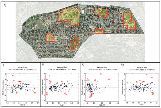
Figure 7.
Observation of unusual residuals (marked in red) from variables most related to LSTw: (a) map of unusual polygons/areas identified in the case study according to residual polygons (indicated in red); (i) residual plot from VLCwL; (ii) residual plot from AvgH; (iii) residual plot from VLCwM; and (iv) residual plot from VCw.
In analysing each variable with LSTs, the results show that the most significant relationships by influence (R2) are as follows: VLCsH, VCs, AvgH, VLCsM, BBAlvar_s, and FSI. Notably, high-level vegetation cover emerges as the most influential variable impacting LSTs, demonstrating a negative association and indicating an increase in high-level correlates with a decrease in LSTs. Similarly, VCs, AvgH, VLCsM, and VCw exhibit negative relationships with LSTs, except for BBAlvar_s, implying that an increase in BBAlvar_s might be linked to higher LSTs (see Table 3). However, the variable associated with low-level vegetation cover shows no significant relationship, contrasting with its influence on LST in winter.

Table 3.
Statistical correlation from simple linear regression of each variable and LSTw_Summer.
In Figure 8, featuring scatterplots, observations reveal that when values surpass 1.0 (more than 20%) in high-level vegetation cover, LSTs values tend to fall below 1 (within LSTs groups of 1 K and −2 K). Conversely, for low-level vegetation cover, values below 2.5 (18%) indicate an increase in LSTs. When VCs values exceed 1.0 (over 45%), only values registering below 0 (within LSTs groups of 0 K and −2 K) are noted. However, for FSI, the trend is reversed, where values below 1.0 (between 0 and 0.35) result in LSTs values above 0.0 (within LSTs groups of 0 K and 5 K). Lastly, for AvgH and BBAlvar_s, which are related to LSTw, no specific patterns were observed.
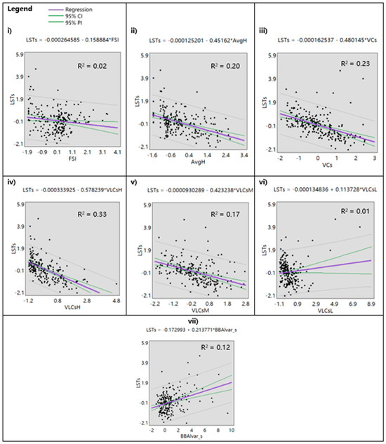
Figure 8.
Scatter plots from simple linear regression of variables with significant relationships with LSTs_Summer: (i) FSI; (ii) AvgH; (iii) VCs; (iv) VLCsH; (v)VLCsM; (vi) VLCsL; and (vii) BBAlvar_s.
In examining unusual residuals for variables with a significant relationship with LSTs, the same areas identified for LSTw—featuring synthetic turf sports fields and a building equipped with photovoltaic cells—are also noted. Furthermore, scattered across the neighbourhood, various polygons share similar characteristics, including single-family buildings at the neighbourhood’s average height and multi-family buildings surpassing the neighbourhood’s average height, coupled with high-level vegetation among the buildings. Figure 9 shows residual plots for the variables most closely associated with LSTs, highlighting these specific areas mentioned earlier.
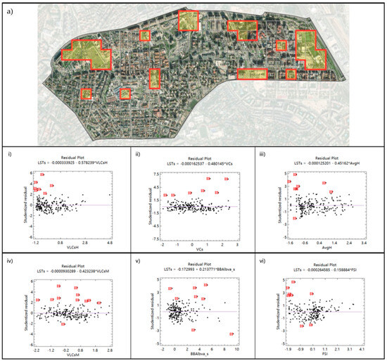
Figure 9.
Observation of unusual residuals (marked in red) from variables most related to LSTs: (a) map of unusual polygons/areas identified in the case study according to residual polygons (indicated in red); (i) residual plot from VLCsH; (ii) residual plot from VCs; (iii) residual plot from AvgH; (iv) residual plot from VLCsM; (v) residual plot from BBAlvar_s; and (vi) residual plot from FSI.
The correlations between seasons show that morphological variables have less correlations with LST in winter. High-, medium-, and general-level vegetation have stronger and more significant correlations with LST in summer than in winter. There is an inverse relationship for low- and high-level vegetation between the seasons. This prompts a discussion on seasonal vegetation priority, where high-level vegetation lacks a significant correlation in winter but exhibits a strong relationship in summer, contrasting with low-level vegetation, which displays a stronger correlation in winter than in summer.
The scatterplot analysis identified specific values signalling significant shifts in LST distributions, allowing precise identification of priority areas based on variable values. Unusual polygons highlighted by the statistical analysis’s adjusted model indicate specific behaviours aligning with multiple variables. These areas should be treated independently due to their deviation from the neighbourhood’s average behaviour validations via higher-resolution orthophotos (0.25 m × 0.25 m per pixel, from the Community of Madrid Directorate General of Urbanism CC-BY 4.0), confirming their distinctions from the neighbourhood’s common characteristics.
4.3. Identitification of Morphological Patterns from Multiple Regression Analysis
Prior to the multiple linear regression analysis, variable correlations were assessed to address multicollinearity concerns. The Pearson correlation matrix (Figure 10) revealed correlations (r < ±0.50) between general vegetation cover and cover by level, considered moderate and strong in Moore, Notz, and Flinger [39]. Consequently, the regressions were conducted without considering general cover variables together with level-specific variables, as these correlations were notable enough to exclude general vegetation cover from the multiple regressions.
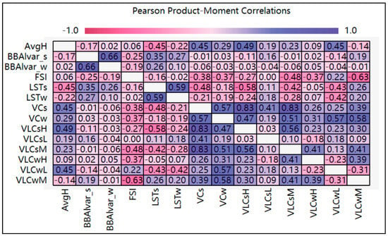
Figure 10.
Pearson product–moment correlations to address multicollinearity concerns between variables.
Table 4 presents results for both fitted models pertaining to the LST’s, including the p-values for each independent variable, R2 values of the model’s explanatory variability for LST’s, the standard error of the estimate (root mean squared error, RMSE), and mean absolute error (MAE).

Table 4.
Results of the multiple regressions applied for the dependent variables LSTw and LSTs.
The regression results in Table 4 highlight the disparity in the number of significant variables describing the distribution of LSTw compared to LSTs. The analysis demonstrates that the derived variables in this study better explain LST in summer as evidenced by the value of R2. Notably, for LSTw, VLCwH variables are suggested, while for LSTs, the six initial variables are considered. In both LSTw and LSTs fitted models, VLCwL and VLCsH emerge as the most influential variables, consistent with Section 4.2. These findings underscore the greater impact of VLCwL on LSTw and VLCsH on LSTs compared to other variables.
From analysis of unusual residuals (outliers), several zones identified in Section 4.2. for LSTw largely coincide with specific areas such as synthetic turf fields, the police building complex, and mixed-use buildings. However, discrepancies arise in LSTs, with new polygons displaying distinct characteristics, emphasising low urban density and different land cover types. Reapplying the backward stepwise selection method, and excluding these unusual polygons, slightly impacts the models’ explanatory power for LSTw and significantly enhances it for LSTs. These results are detailed in Supplementary Material I, Table S1.
Although the morphological variable examined here only explains 20.47% of LSTw and 57.38% of LST distributions, the focus on vegetation cover outweighs built-up characteristics in explanatory power. Comparing the four regressions, low and high vegetation cover levels (VLCwL and VLCsH) exhibit a consistently strong influence on both LST’s. However, the order of influence of vegetation levels shifts between seasons, with medium and low levels influencing LSTw more than high-level vegetation in winter, while the reverse occurs in summer.
To analyse the influence of the variables in LST using the classification made prior to the study [22], four multiple linear regressions for each LST were carried out by separating the polygon data by built-up clusters (a, b, c, and d). The intention was to ascertain variations in variable influence within these clusters, identify better fitting models, and highlight any residual unusual polygons in each cluster. The results reveal VLCwL as the predominant variable in describing LSTw across clusters, with cluster “d” displaying the best fit. In contrast, LSTs values exhibit a dominant influence of VLCsH and VLCsL across clusters, with cluster “a” displaying the best fitting model. Residual polygons largely coincide with LSTs values differing from the mean (0).
Moreover, the observation of unusual polygons within the same clusters reveals critical variations in LST’s due to VLCwL in LSTw and VLCsH in LSTs. This suggests the need for adjustments in the previous classifications to better reflect the impact of these variables. Additionally, buildings exert a greater impact on LSTs than synthetic turf in specific areas consisting of synthetic turf fields and buildings with photovoltaic cell roofs. The detailed results of this analysis can be found in Supplementary Material I, Table S2.
4.4. Characterisation of Morphological Patterns and Distribution of LST
The comparative analysis conducted delineates the similarities and disparities in the results of the developed analyses, focusing on variables that had a greater or lesser influence on the LST’s. Table 5 illustrates the general results derived from comparing the three analyses for LSTw and LSTs, indicating that the pre-existing classifications lack the essential weighting of influential variables necessary to describe the distribution of LSTw and LSTs. Therefore, developing a model that accounts for the influences of these variables on LSTs becomes imperative. This overall comparison presented serves as the initial step toward identifying morphological patterns for a more comprehensive depiction of LSTs’ distribution.

Table 5.
Overall comparison of the results (patterns identified) from the analyses undertaken for LSTw and LSTs.
The results in the preceding sections underline the need to separately consider the influences that each variable has on each LST. As the main objective of this study is to characterise urban biophysical patterns that describe the distribution of LSTs to identify priority areas for intervention, filtered selections of the neighbourhood polygons were proposed based on the biophysical patterns presented in Table 5.
The filtered selections for winter and summer seasons were designed to identify areas likely to exhibit temperatures below and above the neighbourhood average, respectively. For winter, five significant variables influencing LSTw were considered, namely, FSI, AvgH, VLCwL, VLCwM, and BBAlvar_w. In summer, six influential variables associated with LSTs were included: FSI, AvgH, VLCsH, VLCsM, VLCsL, and BBAlvar_s. Table 6 outlines these morphological patterns in order of influence for the filtered polygon selection according to LSTw and LSTs.

Table 6.
Variables considered for the selection of polygons by filter in winter and summer.
From the morphological patterns filtered for winter, 33 polygons were selected within the LSTw groups between the mean (0) and −2 K, coinciding with the lowest measured LST values in the neighbourhood and in agreement with the winter target. The selected polygons represent 47% of the LSTw values in groups −1 K and −2 K, leaving 53% out of that selection.
When considering the unusual polygons (specific areas), the percentage of polygons not selected decreased to 30%. The validation with original LSTw data indicated a partial alignment between the identified morphological patterns and the lowest LSTw values. Figure 11 illustrates the mapping of the selected polygons, unusual areas, and the original LSTw clusters for validation.
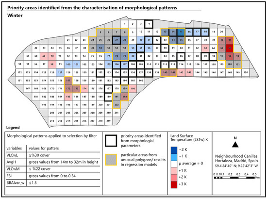
Figure 11.
Priority areas identified from the selection by filter of morphological patterns for Winter.
Conversely, for summer, 57 polygons were selected in groups of LSTs between the mean (0) and +3 K, coinciding with high measured values of LSTs in the neighbourhood and missing values in groups +4 K and +5 K in this selection. These polygons represented 43% of the LSTs values in groups +1 K and +5 K, leaving out 57%. When considering unusual polygons, the percentage not selected was reduced to 11%. Validation with the LSTs data showed an alignment of close to 100% between the identified morphological patterns and the highest LSTs. Figure 12 demonstrates the mapping of the selected polygons conforming to the summer morphological patterns.
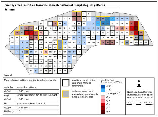
Figure 12.
Priority areas identified from the selection by filter of morphological patterns for Summer.
The resultant maps and percentage representation of selected polygons against those within the groups of LSTw below the mean and LSTs above the mean, indicate the suitability of the defined morphological patterns. These maps reveal additional insights for observation.
5. Discussion
5.1. Methods to Identify Relationships of Biophysical Variabless and LST
The study of the magnitude in which urban factors impact urban climate remains elusive and this type of study contributes to this gap in the field of knowledge [40,41]. To determine the extent to which biophysical characteristics could describe the distribution of LST, we proposed three different methods, aiming for a comprehensive study and comparative analysis. Starting with the parallel observation of the previous classifications and their corresponding group in LST, we found that while this method allowed for a general understanding of their linkage, it presented challenges in pinpointing significant relationships due to the integrated nature of classification variables. Nonetheless, it serves as a starting point for identifying priority areas, especially when considering further steps to uncover precise relationships between characteristics and LST.
Identifying unusual polygons within the same classifications sheds light on the differences in LST values, questioning the efficiency of previous classifications in influencing LST distribution. For instance, in LSTw, certain vegetation characteristics were found to have significant impacts that were overlooked in the initial classification. Similarly, in LSTs, variations in vegetation categories notably affected LST values, emphasising the need for classification adjustments based on vegetation weight, particularly in higher-level categories.
Statistical correlation analysis of the variables separately with LST proved to be more efficient in defining morphological patterns. This method not only identified variables with significant relationships, but also delineated their strength and direction, aiding in ranking their influence. Furthermore, scatter plots allowed a detailed examination of data behaviour and value ranges affecting LST alterations. This is consistent with other studies that have applied correlations, which found low relationships of LST with biophysical factors related to albedo, although they stress the importance of including the physical characteristics (materials) of built urban elements [6,42].
Multiple regression analyses reinforced previous results and revealed distinct outcomes between winter and summer. While this method can be more complex due to requiring prior correlation identification, these analyses showed the capacity of variables to describe LST. Notably, the variables exhibit greater descriptive potential for LSTs compared with LSTw, indicating the need for additional variables for LSTw in future studies.
We observed that most of the analyses carried out on this subject have applied correlation analyses, spatial autocorrelations to identify hot–cold spots, or regression tree models for cluster characterisation [42,43]. However, the approach shown in this study also allows an overall understanding of the behaviour of the study area according to each of the biophysical factors. In this way, the possibility of applying this approach to study other underlying conditions in local urban environments could be expanded.
5.2. Morphological Pattern Characterisation from Biophysical Variables and Identification of Priority Areas
After validating the characterised patterns from the original LST values, the significance of examining detailed vegetation aspects beyond general cover for more accurate LST descriptions was underscored, as mentioned in other studies that have only considered general NDVI, as well as studies of vegetation typologies (arboreal or herbaceous) for the characterisation of urban landscapes [14,42,44].
These identified patterns serve as templates for intervention strategies, particularly concerning LST conditions above or below average during critical climatic seasons. The integration of biophysical characteristics into the patterns becomes necessary, as has been shown in studies where factors linked to Outdoor Thermal Comfort (OTC) and UHI are evaluated separately, thus demonstrating their influence on LST and urban climate [6,11]. The replicability of these diagnoses and interventions proves vital for rapidly evolving urban environments.
Distinctive areas identified through the analyses, notably the particular areas, are crucial due to their significant impact despite not aligning with defined morphological patterns alone. These areas, contributing to a notable portion of LST outliers, demand attention, suggesting their relevance in specific issues within the neighbourhood. This analysis also unveils areas exhibiting seasonal adaptability, visible through changes from winter to summer in LST values. These areas prompt detailed examination of raw biophysical characteristic values to ascertain their influence on adaptive potential, paving the way for questions related to climate regulation, mitigating UHI effects, energy concentration zones, and more.
Figure 13 illustrates comparisons between two areas exhibiting potential adaptability to those identified as priority areas in winter and summer. The aim of this comparison is to show the practical application of the study outcomes, enabling a detailed examination of biophysical characteristics that influence the LST values and their adaptability to the climatic conditions in winter and summer.
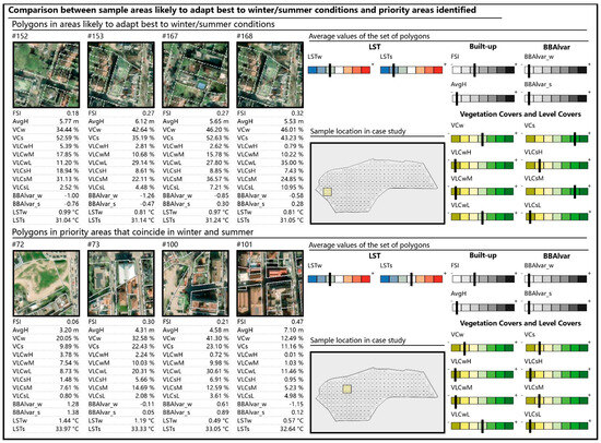
Figure 13.
Comparison between a sample of potentially better adapted areas to winter and summer conditions compared to a sample of priority areas identified from morphological patterns.
The comparison revealed significant changes in general coverage and levels in summer where we see that there is a difference between the two sample areas of up to 3 K. Conversely, the built-up and broadband albedo variables between the two areas show that the vegetation variables have a greater influence. Finally, the most substantial variations between areas were observed in general vegetation and medium-level covers during summer.
5.3. Limitations Found in the Study
The limitations found in the study refer to the variables that were calculated, the results obtained from the analyses, the morphological patterns characterised and, finally, the identification of priority areas.
The consideration of variables in the study shows the necessity to incorporate additional characteristics, particularly to explain the distribution of LSTw, where the adjusted models exhibit a constrained explanatory capacity. While these percentages in the models are not limitations per se, they signify an opportunity for future studies to integrate other unexplored biophysical variables, thereby enhancing the comprehensiveness of the analysis.
Other biophysical factors that can already be obtained from the satellite imagery processes and could be included in the analysis for the identification of patterns, if databases such as cadastres are not available, are indices such as the Normalised Differential Built-up Index (NDBI) and the Soil Adjusted Vegetation Index (SAVI) [40,41,42].
On the other hand, we see that the study is limited to the analysis of daytime LST, not including the variation of LST during the day, which would also be related to the study of biophysical characteristics. Therefore, the results shown here solely encapsulate daytime LST, and may potentially differ if applied to nocturnal LST. Incorporating night-time LST values would imply the acquisition of satellite images corresponding to those times and with resolutions similar to those used in this study.
These limitations highlight the importance of expanding future studies by broadening the scope of variables, incorporating nocturnal LST observations, and interpreting unusual outcomes as valuable insights into unique urban conditions.
6. Conclusions
The study highlights the role of biophysical characteristics in urban settings and the relationships they represent with various conditions, whether linked to environmental or socio-economic dimensions. Examining these characteristics and LST from the three distinct analyses applied allowed the location of intervention areas coinciding with morphological patterns that have an impact on the reduced values of LST in winter and the rising values of LST in summer, in a Mediterranean context.
The study stresses the significance of exploring vegetation dimensions beyond general coverage levels. This indicates the value of studies that consider spatial–temporal scales, where, in varying climatic conditions throughout the year, the understanding of changes in urban biophysical characteristics becomes imperative.
In doing so, we emphasise the need to develop methods to describe urban morphology in a comprehensive manner, not only considering the built elements, but also the natural elements, as there are now more possibilities for measurement, such as remote sensing tools and multisource datasets. This study sets a precedent for the development of methods that are applicable to various urban landscapes.
Supplementary Materials
The following supporting information can be downloaded at: https://www.mdpi.com/article/10.3390/cli12010004/s1, Table S1: Results of the multiple regressions applied for the dependent variables LSTw and LSTs excluding the polygons corresponding to unusual residuals; Table S2: Results of multiple regressions applied to built-up clusters for LSTw and LSTs; Supplementary Material I: Supplementary data with abbreviations and tables mentioned throughout the text (Tables S1 and S2).
Author Contributions
Conceptualization, K.A.G.-P.; methodology, K.A.G.-P., S.D.-A. and D.M.-R.; software, K.A.G.-P.; validation, K.A.G.-P.; formal analysis, K.A.G.-P., S.D.-A. and D.M.-R.; investigation, K.A.G.-P., S.D.-A., D.M.-R. and J.R.G.-C.; resources, K.A.G.-P. and J.R.G.-C.; data curation, K.A.G.-P.; writing—original draft preparation, K.A.G.-P.; writing—review and editing, K.A.G.-P., S.D.-A. and D.M.-R.; visualization, K.A.G.-P.; supervision, S.D.-A., D.M.-R. and J.R.G.-C.; funding acquisition, S.D.-A. and D.M.-R. All authors have read and agreed to the published version of the manuscript.
Funding
The study was also supported by the CONAHCYT-CULTURA Foreign Scholarships in Mexico (Consejo Nacional de Humanidades, Ciencias y Tecnologías-Fondo Nacional para la Cultura y las Artes es un organismo público del gobierno federal mexicano, adscrito al Consejo Nacional para la Cultura y las Artes; ref: 021-000008-01EXTF-00174). The satellite imagery was obtained from the Contratos Menores provided by the TEP 130 Research Group (Arquitectura, Patrimonio y Sostenibilidad: Acústica, Iluminación y Energía). Pléiades imagery was obtained from © CNES (2022), Distribution Airbus DS Geo SA under an Academic License Agreement.
Data Availability Statement
The data in this study are available within the article or its Supplementary Materials.
Acknowledgments
The authors would like to thank the editors and the anonymous reviewers for their time and efforts reviewing this manuscript.
Conflicts of Interest
The authors declare no conflicts of interest.
References
- NOOA National Oceanic and Atmospheric Administration. April 2023 Was Earth’s Fourth Warmest on Record. Available online: https://www.noaa.gov/news/april-2023-was-earths-fourth-warmest-on-record (accessed on 12 May 2023).
- Kamal-Chaoui, L.; Robert, A. (Eds.) Competitive Cities and Climate Change; OECD Regional Development Working Papers N° 2; OECD Publishing, ©OECD: Paris, France, 2009. [Google Scholar]
- Kousis, I.; Pigliautile, I.; Pisello, A.L. Intra-urban microclimate investigation in urban heat island through a novel mobile monitoring system. Sci. Rep. 2021, 11, 9732. [Google Scholar] [CrossRef] [PubMed]
- Bowler, D.E.; Buyung-Ali, L.; Knight, T.M.; Pullin, A.S. Urban greening to cool towns and cities: A systematic review of the empirical evidence. Landsc. Urban Plan. 2010, 97, 147–155. [Google Scholar] [CrossRef]
- Hoelscher, M.-T.; Nehls, T.; Jänicke, B.; Wessolek, G. Quantifying cooling effects of facade greening: Shading, transpiration and insulation. Energy Build. 2016, 114, 283–290. [Google Scholar] [CrossRef]
- Kalogeropoulos, G.; Dimoudi, A.; Toumboulidis, P.; Zoras, S. Urban Heat Island and Thermal Comfort Assessment in a Medium-Sized Mediterranean City. Atmosphere 2022, 13, 1102. [Google Scholar] [CrossRef]
- Stewart, I.D.; Oke, T.R. Local Climate Zones for Urban Temperature Studies. Bull. Am. Meteorol. Soc. 2012, 93, 1879–1900. [Google Scholar] [CrossRef]
- Chapman, S.; Watson, J.E.M.; Salazar, A.; Thatcher, M.; McAlpine, C.A. The impact of urbanization and climate change on urban temperatures: A systematic review. Landsc. Ecol. 2017, 32, 1921–1935. [Google Scholar] [CrossRef]
- Gómez-Baggethun, E.; Barton, D.N. Classifying and valuing ecosystem services for urban planning. Ecol. Econ. 2013, 86, 235–245. [Google Scholar] [CrossRef]
- Masson, V.; Heldens, W.; Bocher, E.; Bonhomme, M.; Bucher, B.; Burmeister, C.; de Munck, C.; Esch, T.; Hidalgo, J.; Kanani-Sühring, F.; et al. City-descriptive input data for urban climate models: Model requirements, data sources and challenges. Urban Clim. 2020, 31, 100536. [Google Scholar] [CrossRef]
- Aghamolaei, R.; Azizi, M.M.; Aminzadeh, B.; O’donnell, J. A comprehensive review of outdoor thermal comfort in urban areas: Effective parameters and approaches. Energy Environ. 2022, 34, 2204–2227. [Google Scholar] [CrossRef]
- Li, H.; Liu, Y.; Zhang, H.; Xue, B.; Li, W. Urban morphology in China: Dataset development and spatial pattern characterization. Sustain. Cities Soc. 2021, 71, 102981. [Google Scholar] [CrossRef]
- Yu, D.; Fang, C. Urban Remote Sensing with Spatial Big Data: A Review and Renewed Perspective of Urban Studies in Recent Decades. Remote Sens. 2023, 15, 1307. [Google Scholar] [CrossRef]
- Noblejas, H.C.; Orellana-Macías, J.M.; Rodríguez, M.F.M. Use of Vegetation to Classify Urban Landscape Types: Application in a Mediterranean Coastal Area. Land 2022, 11, 228. [Google Scholar] [CrossRef]
- Grove, M.; Cadenasso, M.L.; Burch, W.R., Jr.; Prickett, S.T.A.; Schwarz, K.; Wilson, M.; Troy, A.; Boone, C., Jr. Data and methods comparing social structure and vegetation structure of urban neighborhoods in Baltimore, Maryland. Soc. Nat. Resour. 2006, 19, 117–136. [Google Scholar] [CrossRef]
- Pandey, P.C.; Balzter, H.; Srivastava, P.K.; Petropoulos, G.P.; Bhattacharya, B. 21—Future perspectives and challenges in hyperspectral remote sensing. Hyperspectral Remote Sens. 2020, 429–439. [Google Scholar]
- García-Pardo, K.A.; Moreno-Rangel, D.; Domínguez-Amarillo, S.; García-Chávez, J.R. Remote sensing for the assessment of ecosystem services provided by urban vegetation: A review of the methods applied. Urban For. Urban Green. 2022, 74, 127636. [Google Scholar] [CrossRef]
- McGee, J.A.; Day, S.D.; Wynne, R.H.; White, M.B. Using geospatial tools to assess the urban tree canopy: Decision support for local governments. J. For. 2012, 110, 275–286. [Google Scholar] [CrossRef]
- Hostetler, A.E.; Rogan, J.; Martin, D.; DeLauer, V.; O’neil-Dunne, J. Characterizing tree canopy loss using multi-source GIS data in Central Massachusetts, USA. Remote Sens. Lett. 2013, 4, 1137–1146. [Google Scholar] [CrossRef]
- Huang, C.; Ye, X.; Deng, C.; Zhang, Z.; Wan, Z. Mapping above-ground biomass by integrating optical and SAR imagery: A case study of Xixi National Wetland Park, China. Remote Sens. 2016, 8, 647. [Google Scholar] [CrossRef]
- Wang, J.; Gao, C.; Wang, M.; Zhang, Y. Identification of Urban Functional Areas and Urban Spatial Structure Analysis by Fusing Multi-Source Data Features: A Case Study of Zhengzhou, China. Sustainability 2023, 15, 6505. [Google Scholar] [CrossRef]
- García-Pardo, K.A.; Moreno-Rangel, D.; Domínguez-Amarillo, S.; García-Chávez, J.R. Urban classification of the built-up and seasonal variations in vegetation: A framework integrating multisource datasets. Urban For. Urban Green. 2023, 89, 128114. [Google Scholar] [CrossRef]
- Ayuntamiento de Madrid. Distrito en cifras (Información de Barrios). 1 January 2022. Available online: https://www.madrid.es/portales/munimadrid/es/Inicio/El-Ayuntamiento/Estadistica/Areas-de-informacion-estadistica/Economia/Distritos-en-cifras-Informacion-de-Barrios-/ (accessed on 18 August 2022).
- Boletín Oficial del Estado. 1949. DECRETO de 17 de Agosto de 1949 por el que se Aprueba la Anexión Total del Término Municipal de Canillas al de Madrid. B. O. del E.—Núm. 319. Available online: https://www.boe.es/da-tos/pdfs/BOE/1949/319/A04782-04782.pdf (accessed on 10 January 2020).
- Fernández García, A. La Evolución social de Madrid en la época Liberal (1834–1900). In Ciclo de Conferencias Arquitectura u Espacio Urbano de Madrid en el siglo XIX; Museo de Historia de Madrid: Madrid, Spain, 2008; pp. 10–29. Available online: https://www.madrid.es/ (accessed on 10 January 2020).
- Zhao, M.; Cai, H.; Qiao, Z.; Xu, X. Influence of urban expansion on the urban heat island effect in Shanghai. Int. J. Geogr. Inf. Sci. 2016, 30, 2421–2441. [Google Scholar] [CrossRef]
- Chen, Y.; Yang, J.; Yu, W.; Ren, J.; Xiao, X.; Xia, J.C. Relationship between urban spatial form and seasonal land surface temperature under different grid scales. Sustain. Cities Soc. 2023, 89, 104374. [Google Scholar] [CrossRef]
- Han, L.; Lu, L.; Fu, P.; Ren, C.; Cai, M.; Li, Q. Exploring the seasonality of surface urban heat islands using enhanced land surface temperature in a semi-arid city. Urban Clim. 2023, 49, 101455. [Google Scholar] [CrossRef]
- Han, S.; Hou, H.; Estoque, R.C.; Zheng, Y.; Shen, C.; Murayama, Y.; Pan, J.; Wang, B.; Hu, T. Seasonal effects of urban morphology on land surface temperature in a three-dimensional perspective: A case study in Hangzhou, China. J. Affect. Disord. 2023, 228, 109913. [Google Scholar] [CrossRef]
- Zhou, Y.; Li, X.; Chen, W.; Meng, L.; Wu, Q.; Gong, P.; Seto, K.C. Satellite mapping of urban built-up heights reveals extreme infrastructure gaps and inequalities in the Global South. Proc. Natl. Acad. Sci. USA 2022, 119, 46. [Google Scholar] [CrossRef]
- Jiménez-Espada, M.; García, F.M.M.; González-Escobar, R. Urban Equity as a Challenge for the Southern Europe Historic Cities: Sustainability-Urban Morphology Interrelation through GIS Tools. Land 2022, 11, 1929. [Google Scholar] [CrossRef]
- Rahman, H.; Islam, H.; Neema, M.N. GIS-based compactness measurement of urban form at neighborhood scale: The case of Dhaka, Bangladesh. J. Urban Manag. 2022, 11, 6–22. [Google Scholar] [CrossRef]
- Liu, B.; Deng, Y.; Li, M.; Yang, J.; Liu, T. Classification Schemes and Identification Methods for Urban Functional Zone: A Review of Recent Papers. Appl. Sci. 2021, 11, 9968. [Google Scholar] [CrossRef]
- Sobrino, J.A.; Jiménez-Muñoz, J.C.; Paolini, L. Land surface temperature retrieval from LANDSAT TM 5. Remote Sens. Environ. 2004, 90, 434–440. [Google Scholar] [CrossRef]
- García, D.H. Evaluation and Analysis of the Effectiveness of the Main Mitigation Measures against Surface Urban Heat Islands in Different Local Climate Zones through Remote Sensing. Sustainability 2023, 15, 10410. [Google Scholar] [CrossRef]
- Aryal, J.; Sitaula, C.; Aryal, S. NDVI threshold-based urban green space mapping from sentinel-2A at the Local Governmental Area (LGA) level of victoria, Australia. Land 2022, 11, 351. [Google Scholar] [CrossRef]
- Balaguer-Beser, Á.A.; Ruiz-Fernández, L.Á. Selección de un modelo de regresión lineal múltiple para el cálculo de la precipitación media en verano. Universitat Politècnica de València. 2021. Available online: http://hdl.handle.net/10251/167659 (accessed on 13 November 2023).
- Berman, J.J. Chapter 4—Understanding Your Data. In Data Simplification; Kaufmann, M., Ed.; Morgan Kaufmann: Boston, MA, USA, 2016; pp. 135–187. ISBN 9780128037812. [Google Scholar] [CrossRef]
- Moore, D.S.; Notz, W.I.; Flinger, M.A. The Basic Practice of Statistics, 6th ed.; W. H. Freeman and Company: New York, NY, USA, 2013. [Google Scholar]
- Guechi, I.; Gherraz, H.; Alkama, D. Correlation analysis between biophysical indices and Land Surface Temperature using remote sensing and GIS in Guelma city (Algeria). Bull. Société R. Sci. Liège 2021, 90, 158–180. [Google Scholar] [CrossRef]
- Illyani, I.; Azizan, A.S.; Rosmadi, F. Land Surface Temperature and Biophysical Factors in Urban Planning. In Proceedings of the Conference: World Academy of Science, Engineering and Technology, Kuala Lumpur, Malaysia, 29–30 May 2012; Volume 68. [Google Scholar]
- Guo, G.; Wu, Z.; Xiao, R.; Chen, Y.; Liu, X.; Zhang, X. Impacts of urban biophysical composition on land surface temperature in urban heat island clusters. Landsc. Urban Plan. 2015, 135, 1–10. [Google Scholar] [CrossRef]
- Li, D.; Wang, L. Sensitivity of Surface Temperature to Land Use and Land Cover Change-Induced Biophysical Changes: The Scale Issue. Geophys. Res. Lett. 2019, 46, 9678–9689. [Google Scholar] [CrossRef]
- Addas, A. Understanding the Relationship between Urban Biophysical Composition and Land Surface Temperature in a Hot Desert Megacity (Saudi Arabia). Int. J. Environ. Res. Public Health 2023, 20, 5025. [Google Scholar] [CrossRef]
Disclaimer/Publisher’s Note: The statements, opinions and data contained in all publications are solely those of the individual author(s) and contributor(s) and not of MDPI and/or the editor(s). MDPI and/or the editor(s) disclaim responsibility for any injury to people or property resulting from any ideas, methods, instructions or products referred to in the content. |
© 2023 by the authors. Licensee MDPI, Basel, Switzerland. This article is an open access article distributed under the terms and conditions of the Creative Commons Attribution (CC BY) license (https://creativecommons.org/licenses/by/4.0/).
