Article

Towards a Flood Assessment Product for the Humanitarian and Disaster Management Sectors Based on GNSS Bistatic Radar Measurements

by
Nereida Rodriguez-Alvarez
1,* and
Andrew Kruczkiewicz
2,3,4
1
Planetary Radar and Radio Science Group, Jet Propulsion Laboratory, California Institute of Technology, Pasadena, CA 91109, USA
2
International Research Institute for Climate and Society, Climate School, Columbia University, 61 Route 9W, Palisades, NY 10964, USA
3
Red Cross Red Crescent Climate Centre, 2953 HT The Hague, The Netherlands
4
Faculty of Geo-Information Science and Earth Observation, University of Twente, 7514 AE Enschede, The Netherlands
*
Author to whom correspondence should be addressed.
Climate 2022, 10(5), 77; https://doi.org/10.3390/cli10050077
Submission received: 13 April 2022 / Revised: 18 May 2022 / Accepted: 20 May 2022 / Published: 23 May 2022

Abstract

:
This manuscript focuses on the need for tailoring flood assessment products to decision making within the humanitarian sector. Decision-makers often struggle to extract all of the information contained in scientific products, either because they come from different fields of expertise or because they have different needs that are not captured in the results or the processing of the data. Here we define the key elements of a flood assessment product designed for the humanitarian sector. From a remote sensing perspective, in order to assess flooding, the measurement sampling properties, i.e., spatial resolution and temporal repeat, are key. We have therefore implemented a methodology through the processing and interpretation of the measurements from the Cyclone Global Navigation Satellite System (CYGNSS) mission. CYGNSS measurements are usually parametrized in various possible observables. Those observables are then linked to the surface characteristics, such as, in this case, the presence of inundation in the CYGNSS footprint. Our methodology includes the variability of the pixels in landscapes with infrastructure, rivers, agricultural fields, rural areas, and other elements characteristic of the agricultural-urban interface. We provide an original methodology that uses CYGNSS mission bistatic radar measurements and an artificial intelligence classification algorithm based on statistical properties of the land pixels through a k-means clustering strategy to detect and monitor flooding events, as well as to characterize the land surface prior to and post flooding events. The novel methodology to derive a flooding product is then evaluated towards the needs of the humanitarian sector by a cognizant link (a translator) between technologists or scientists and decision-makers. The inclusion of humanitarian needs into product development following the advice of a cognizant link is novel to the applications developed employing GNSS bistatic radar data.

1. Introduction

On a global scale, floods are one of the most devastating natural hazards. The term flood includes riverine floods, when the flooding is caused by overflown rivers; pluvial floods, when the primary cause is intense rain that the ground cannot absorb; flash floods, when flooding originates rapidly in low-lying areas; urban floods, when the cause is a lack of drainage in an urban area; coastal floods, which originate from seawater covering land areas; and glacial lake outburst floods, when the dam containing a glacial lake fails [1,2,3,4]. This manuscript focuses on floods impacting the human-natural interface, directly and indirectly, leading to high casualty levels and causing losses of billions of US dollars in various sectors, including agriculture, health, energy, transportation, and communications [5]. The agricultural-urban interface, comprising urban, peri-urban, and agricultural areas, is affected by most types of floods, including riverine, pluvial, urban, and flash floods. However, the impact from different types of floods varies significantly.
Flash floods, in particular, have a damage profile that is different from riverine floods, causing more sudden impacts over a variety of socioeconomic contexts [6]. Further, compared to other types of floods, flash floods are more likely to occur outside of areas that are traditionally considered to be at high risk of riverine flooding, leading to a situation where some populations at risk may not appropriately perceive their risk, leading to challenges in developing early warning systems that influence anticipatory action to be taken [7]. Riverine floods occur in known floodplains when prolonged rainfall over several days, intense rainfall over a short period of time, or a debris jam causes a river or stream to overflow and flood the surrounding area. Severe thunderstorms can bring heavy rain in the spring and summer; or tropical cyclones can bring intense rainfall in the summer and fall to coastal states causing coastal floods and to inland states causing riverine, urban, and pluvial floods. Key drivers of floods are rainfall intensity (rate of rainfall), duration (how long the rain lasts), topography, soil conditions, and ground cover. Some of the floods that have occurred in recent years are summarized in Table 1.
The fast-changing conditions that increase flood risk are difficult to monitor with most of the existing satellite remote sensing instruments primarily due to limitations in temporal and spatial resolution, cloud cover, shadows and repeat cycle [8]. Adequate characterization of floods at the agricultural-urban interface requires moderate to high spatial resolution (~1 km) and daily to sub-daily measurements [9]. There are several microwave remote sensing systems that have the potential to fulfil those requirements and, in addition, can see the surface regardless of almost any type of weather, day or night conditions, such as L-band radar, synthetic aperture radar and radiometers [10]. In general, the signals from microwave sensors can penetrate through the medium, up to some degree dependent on the frequency of operation of the instrument and therefore have the potential to detect flooded conditions underneath the vegetation canopy [10]. Current operational microwave capabilities to characterize flooding rely on either scatterometers or radiometers, such as the Special Sensor Microwave Imager (SSM/I, K- and Ka-band, [11]), the Soil Moisture Ocean Salinity (SMOS, L-band, [12]) and the SMAP (L-band, [13]), that provide observations with a 3-day repeat cycle at coarse scales (~25–50 km), or SAR’s, such as Sentinel-1 (C-band, [14]) or the Phased Array L-band Synthetic Aperture Radar (PALSAR-2, L-band, [15]) that provides high resolution (< 100 m) imagery at lower repeat cycles of 12 to 14 days. None of those missions fully satisfy all the requirements for implementing a flood product, much less a flash flood product, whose characteristics are even more challenging: sudden, quicker, and occurring in unexpected areas. In general, the detection of features rapidly evolving would benefit from the availability of measurements with high repeat. L-band GNSS bistatic radar signals are an ideal set of measurements to complement the limitations of the above-mentioned instruments and are key to assessing rapidly evolving features. There are some operational products for global flood prediction and warning based on weather prediction coupled with increasingly accurate satellite observations and hydrological models, such as [16] based on models and precipitation measurements from the Rainfall Measuring Mission (TRMM, [17]) Multi-satellite Precipitation Analysis (TMPA), or operational products for global flood mapping and damage assessment based on observed satellite time series records of flood events and modelling, such as the Near Real Time (NRT) Moderate Resolution Imaging Spectroradiometer (MODIS) Flood Mapping [18] based on MODIS-based algorithm developed in [19] or, as another example, the Advanced Rapid Imaging and Analysis (ARIA, [20]) project based on Sentinel 1 A/B, space-based geodetic measurement from Interferometric Synthetic Aperture Radar (InSAR), and Differential Global Positioning System (DGPS). Data from the 8 satellites that form CYclone Global Navigation Satellite System (CYGNSS) mission’s constellation [21,22] have also been employed in several spatial assessment studies, such as [23] that provides an assessment of recently updated products to feature a novel calibration approach that includes the capability to exploit data collected from the zenith front-end to account for the variability of available GPS power. The study in [24] showed an image processing algorithm leveraging the surface reflectivity signal to produce a water mask of inland waterbodies at 0.01° × 0.01° spatial resolution. Research has been conducted demonstrating the technical and scientific merit of the CYGNSS dataset for flood detection. For example, measurements taken from CYGNSS during the 2017 Atlantic hurricane season suggested that the flooding event occurring in Texas from Hurricane Harvey was well captured by the GNSS-R signals. The effect of both Hurricane Irma affecting Cuba and Hurricane Harvey affecting Texas was clearly noted by the CYGNSS measurements [25]. CYGNSS data is averaged over a certain grid pre-event (1 July to 20 August 2017) and during the whole storm period (25 August–15 September 2017). The observed change in surface reflectivity is classified as inundation by simple thresholding. Similarly, authors in [26] analyze CYGNSS data over China, proving the ability of those measurements to capture the dynamics of flood inundations caused by six typhoon events from July to September 2017.
The characterization of flooding at the agricultural-urban interface, including detection and monitoring of its dynamics on a daily basis, would provide an important source of information and a step towards better decision-making strategies from risk management agencies, helping protect population and infrastructure, and would promote disaster risk reduction policies as noted in the Sendai Framework [27].
This manuscript is structured as follows: Section 2 provides the background for the relevance of the collaboration between technology, science, and the humanitarian sectors.
Section 3 provides the main body of the manuscript where we explain the methodologies employed in our flood product and test it over two case studies:
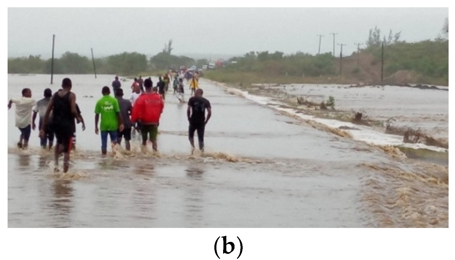
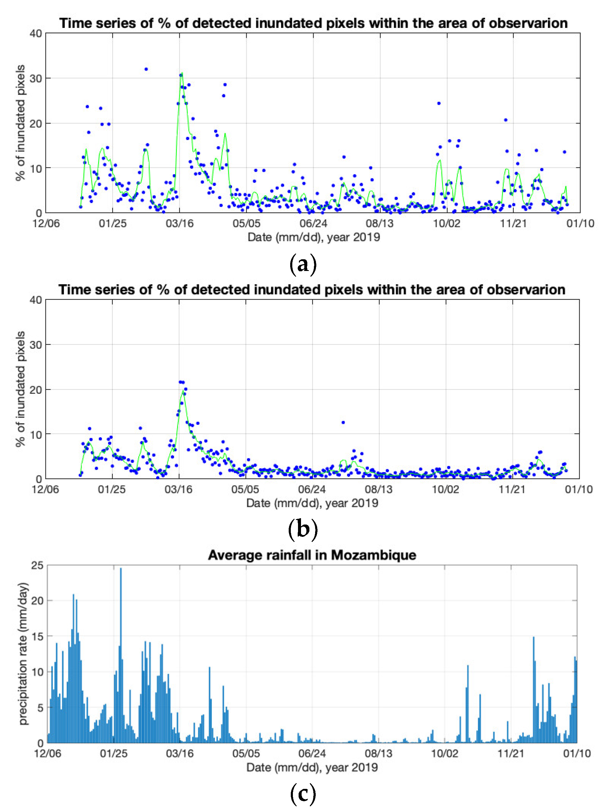
  • The Mozambique floods in 2019, caused by two consecutive tropical cyclones (Idai and Kenneth), leading to casualties, however, the majority were not caused by the storm surge flooding, but rather by both inland riverine flooding and urban/peri-urban flash flooding days after landfall [28];
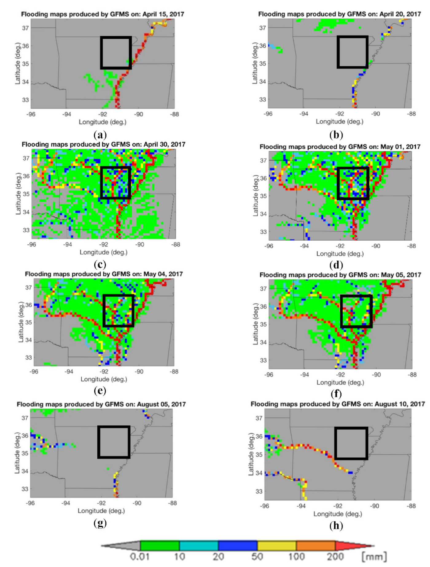
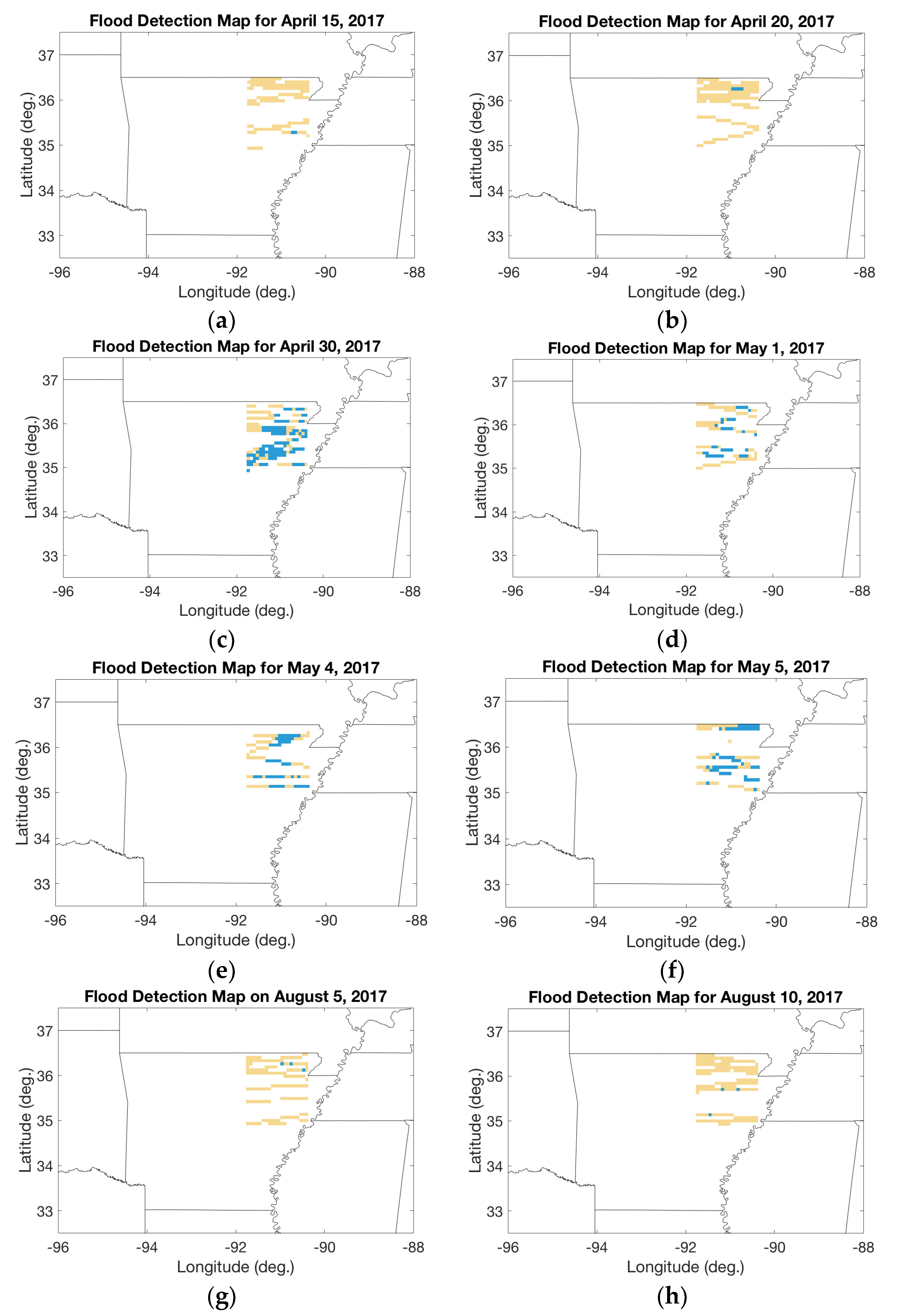
  • The Midwest spring floods in 2017, an example of pluvial floods where the primary cause was recurrent intense rain that the ground could not absorb.
Section 4 provides a description of the humanitarian components. Section 5 provides discussions on the usefulness of signals-of-opportunity for the flood application and on the benefits of multi-sensor information. Section 6 provides the conclusions for the work presented.

2. The Collaboration between Technology, Science, and the Humanitarian Sectors

Many products that indicate flood extent or flood risk are currently produced, but those products are usually not tailored to the needs of decision-makers on the ground. In order to make those products effective, communicating the scientific information to decision-makers in the humanitarian sector requires appropriate tailoring and brokering to increase the likelihood of the data being integrated into policy development or decision-making [29]. To accomplish this, the humanitarian sector needs to be involved in the development of such products so they can be adapted to specific events and to the specific needs of decision-makers [30].
Universities or research centers are one of the sources of flood product development, but given the nature of those types of institutions, many lack the mandates and incentive structures to support operational decision making in the humanitarian and development sector. Promoting structured and mutually beneficial collaboration between research and humanitarian communities is a critical element in developing a comprehensive flood product that can inform flood preparedness, response, recovery, and resilience [31]. Doing so will contribute to a better understanding of the floods and their socioeconomic impact, in particular flash floods—which have been historically difficult to assess [32]. Further, from a disaster management and preparedness perspective, outputs could have a significant impact on the humanitarian sector-wide movement towards anticipatory action before a flood disaster occurs, as they can be considered as candidate datasets during trigger development [33]. Strategic collaboration between institutions will also benefit from direct connections to the humanitarian sector, which will help towards developing better strategies to improve decision-makers’ understanding of floods and how to prioritize the populations at highest risk of flood impact [34,35]. The presented work helps to better characterize the dynamics of the Earth’s surface, improving the capability to assess and respond to floods, and contributes towards the use of Earth system science research for societal benefit [36,37]. Our work uses space-based bistatic radar measurements to provide flood-related information, not fully characterized by other remote sensing instruments, and more generally, to open the integration of these signals into retrieval algorithms, easing the analysis of their impact.

3. The Technological and Science Component

In this section, we focus primarily on the methodologies employed to build our flood detection and monitoring algorithms to generate the flood product. We have developed the algorithms, shaping them to satisfy the needs of the humanitarian sector. These needs were informed by a translator, an entity that understands decision-makers’ needs and has enough background to translate those needs to scientists and technologists, and therefore is able to provide a number of specific requirements:
  • Temporal resolution in the order of 1 day. This is key to capturing fast-occurring events, such as flash floods.
  • Spatial resolution in the order of 500 m to 1 km. This is key to capturing flooding events at a local scale.
  • Selecting measurement directly linked to the presence of standing water.
  • Analyze the landscapes in terms of their unique characteristics.
  • Use the feedback from the humanitarian sectors to flag false positives from the TSH flood product.
  • Provide the number of pixels flooded in a certain area.
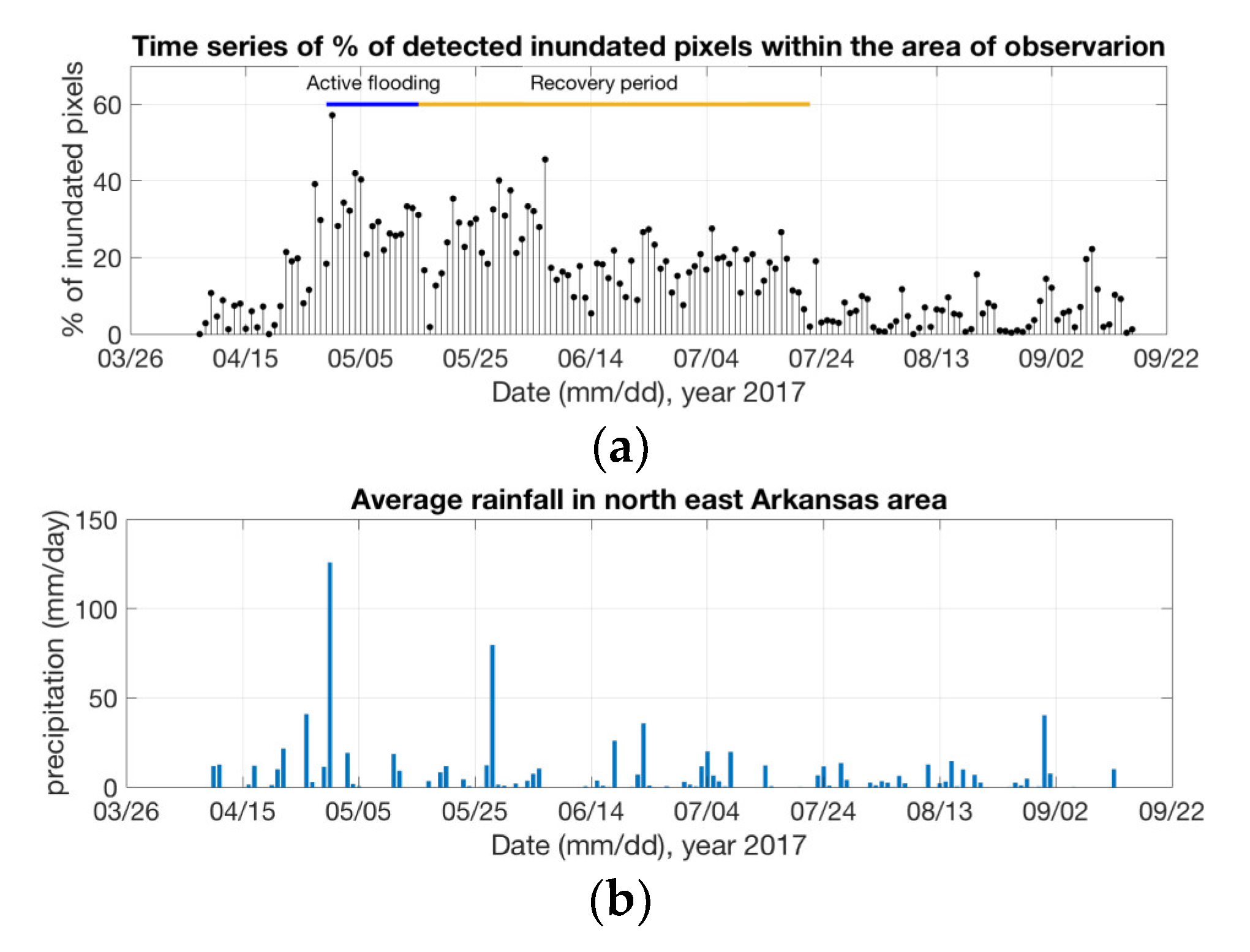
  • Correlate the inundated pixels with precipitation events in the area.
  • Provide a way to understand how the soil is recovered from a flood.
The sub-sections describe the bistatic radar data, the primary dataset allowing to comply with the above requirements. We analyze both spatial and temporal resolution of the data. The algorithm is defined and explained in detail followed by the processing done over different areas in two case examples, showing the ability of the algorithm to detect and monitor floods, as well an example of validation analysis.

3.1. Technology: The Bistatic Radar Dataset

Sampling needs for pluvial floods are even more demanding than what is sufficient for other types of flooding, such as wetlands or coastal flooding, where the events can be observed during weeks or months (wetlands) and occupying 100s of kilometers (massive events due to hurricanes). Currently, the bistatic radar measurements from the CYGNSS [21,22] mission are the most suitable for short duration pluvial floods. CYGNSS is a constellation of 8 satellites with capability of receiving the signals from the Global Positioning System (GPS) as those bounce of the Earth’s surface. CYGNSS tracks up to 4 specular points per receiver resulting on 32 simultaneous measurements per second. The number of measurements per second gathered by CYGNSS provides a coverage and a sampling repeat that surpasses any other GNSS bistatic radar measurement currently available. CYGNSS measurements are usually parametrized in various possible observables which are then linked to the surface characteristics, such as in this case, the presence of inundation in the CYGNSS footprint. This intrinsic aspect of the bistatic radar observable makes CYGNSS data ideal to satisfy one of the key requirements set by the translator; the measurement directly linked to the presence of standing water. The specific observables selected in our methodology are further described in Section 3.2. Aside from CYGNSS there is no current bistatic radar mission that can provide similar performance. Table 2 shows the TechDemoSat-1 mission (TDS-1, [38]) and SMAP radar receiver or SMAP Reflectometer [39,40,41,42].
Previous works have made assumptions on the scattering area size of GPS signals bouncing off inundated areas. When signals are scattered from inundated areas, where the surface is near flat, the coherent scattering component dominates the signal reflection and the area where the signals are scattered from can be ideally assumed to be that of the first Fresnel zone. The first Fresnel zone is defined as and ellipse whose semi-minor and semi-major axis are a function of the distances between the transmitter, the receiver, and the specular point, as well as the wavelength of the scattered signal, and it is oriented with its semi-major axis in the transmitter-to-receiver direction. In [43], the authors provided the calculations for the size of the scattering area for CYGNSS reflections accounting for the integration time. Those calculations indicate the scattering area at each specular point has a size between [0.6 km × 6.6 km] and [1 km × 8.8 km] or [6.6 km × 0.6 km] and [2.8 km × 7 km], for the [cross track × along track] direction, depending both on the incidence angle and the relative orientation of the first Fresnel zone, with its semi-major axis oriented towards the transmitter-to-receiver direction, and the along-track direction. In reality, the scattering area of inundated areas extends beyond the first Fresnel zone, causing the above assumption to introduce errors. To infer the scattering area size of individual measurements, the authors in [41] provide the true spatial resolution of CYGNSS-like measurements. As it was shown in [41], for wetlands, the spatial resolution could reach up to 2.8 km, as both the presence of vegetation and surface winds have an impact on the scattering [44]. In addition, CYGNSS has modified the raw data processing to reduce the integration time to 0.5 s which reduces the elongation of the ellipses due to the integration time, i.e., the scattering area from where reflections are coming from, to 3 km. The spatial resolution assigned to CYGNSS measurements should be revised respect to those generally assumed in order studies, such as in [41,43].
Summarizing, CYGNSS data obtained at 0.5 s integration time is the only available dataset that can be obtained at a temporal resolution of 1 day with a spatial resolution in the order of 1 to 3 km. This specification is over what the decision-makers would desire, but given its temporal repeat over the flooded areas, CYGNSS data continues to be key. To comply with both requirements set by the translator, temporal resolution in the order of 1 day and spatial resolution in the order of 500 m to 1 km, CYGNSS data can be merged to synthetic aperture radar data (revisit of 14 days and ~100 m resolution), optical imagery data (limited by clouds), and soil moisture data (3 day revisit and 9 km resolution from Soil Moisture Active Passive—SMAP—mission) to generate a merged product with spatial resolution below 500 m and daily temporal repeat. This is not within the scope of our current work and will be addressed in future investigations.
For our approach, in order to compute the approximate spatial resolution of each measurement, we applied the methodology of Rodriguez-Alvarez et al. 2019 [41]. The spatial resolution of GNSS-R observations is variable and depends on the scattering surface, the incidence angle, and the integration time. The methodology applies to CYGNSS measurements, regardless of the scattering surface and incidence angle [41]. The measurement obtained from a GNSS-R receiver is a delay–Doppler map (DDM), [45,46], which represents the power scattering of the GPS signal over the Earth’s surface collected at different values of delay and Doppler. The general approach to map the DDM information to its native spatial resolution [47,48,49,50] is defined in Appendix A.

3.2. Science: The Bistatic Radar Signal Processing

We first define the selected measurement observables, i.e., trailing edge slope (TES) and peak reflectivity, computed from the measured delay–Doppler map [45,46]. Then we specify the main considerations and steps of the classification algorithm, including gridding, averaging, and classification steps. Then we dedicate a subsection to explaining the main element used for the classification of pixels, which is a k-means clustering [51] algorithm based on grouping samples by their mean as a representation of the properties of the pixels within the scene. Our strategy benefits from the observation of a clear link between the measurement and the presence of standing water in the pixels, i.e., robust to the reflectivity variations typical of the agricultural–urban interface, and analyzes the landscapes in terms of their unique characteristics.

3.2.1. GNSS-R Observables

The GNSS-R measurement obtained from CYGNSS is the delay–Doppler map (DDM) [45,46]. We assume coherency over flooded areas and, as a first approximation, we assume the expression of the coherent reflected power provided in [52] as:
P r x = Γ P T X λ 2 G T X G R X 4 π 2 R T X + R R X 2
where R T X is the distance between the transmitter and the specular point, R R X is the distance between the specular point and the receiver, G R X is the gain of the receiver antenna in the specular direction, G T X is the gain of the GPS transmitter antenna in the specular direction, P T X is the transmitted power of the GPS, λ is the wavelength of the GPS signal computed as the speed of the light over the GPS frequency 1.57542 GHz, and Γ is the reflectivity of the surface from where the GPS signals scatter.
The CYGNSS mission provides a number of documents describing the calibration levels and the equations applied. In this study, we have utilized the bistatic radar cross-section variable available in the CYGNSS Level 1 version 2.1 dataset (brcs variable in the dataset, P L 1 b ), whose expression is defined in [53], and can be used in combination with Equation (1) to compute the reflectivity DDM ( Γ ) as a function of P L 1 b as:
Γ = R T X + R R X 2 R P L 4 π P L 1 b
The data was filtered following the same quality flag selection as defined in [43,54], and shown for completeness in Appendix C in Table A2.
From Γ several observables can be computed. A description of observables used in this study to retrieve geophysical parameters is provided:
  • The peak value of the reflectivity, which ideally corresponds to the maximum value of the reflectivity and is related to the dielectric properties of the surface.
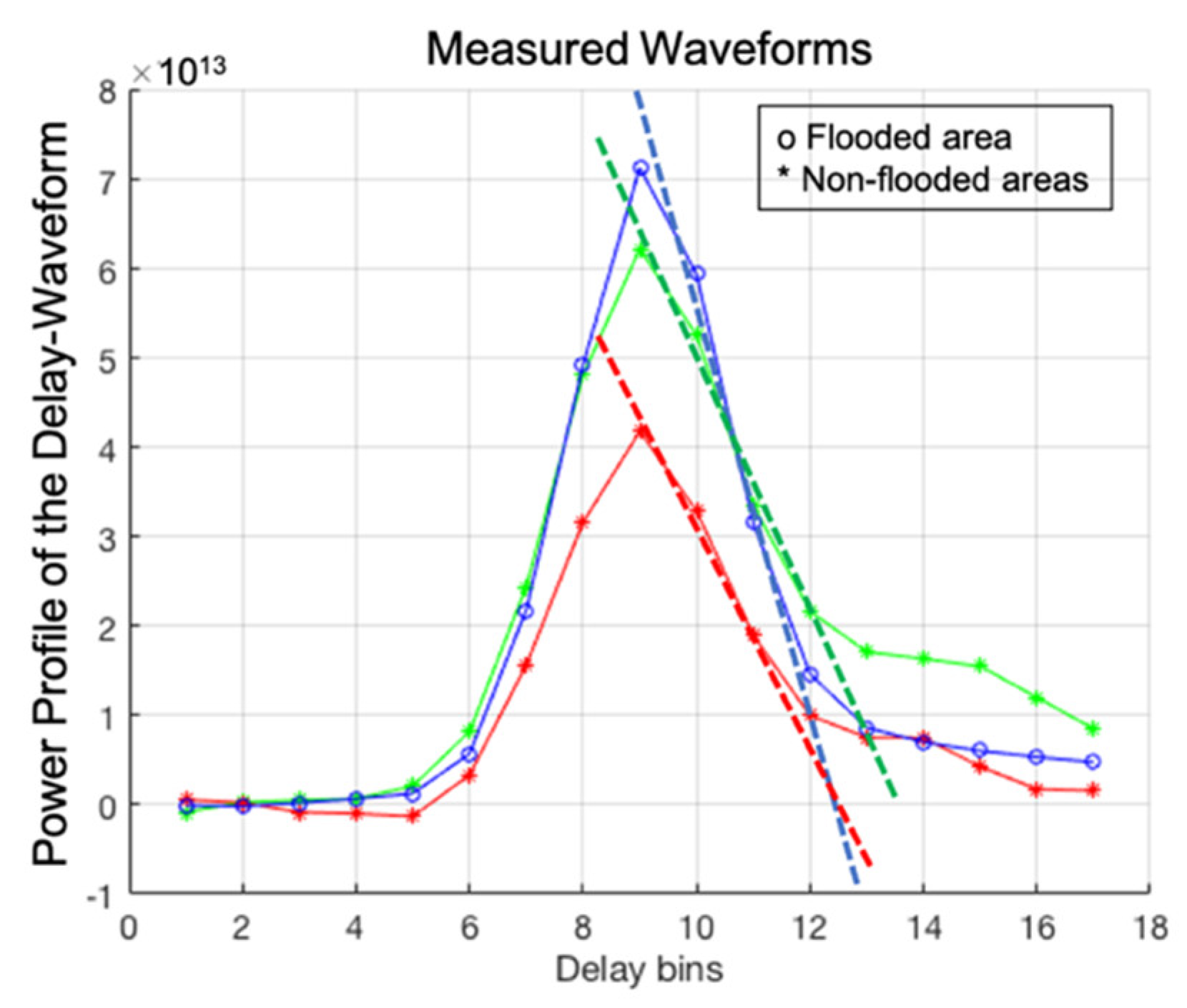
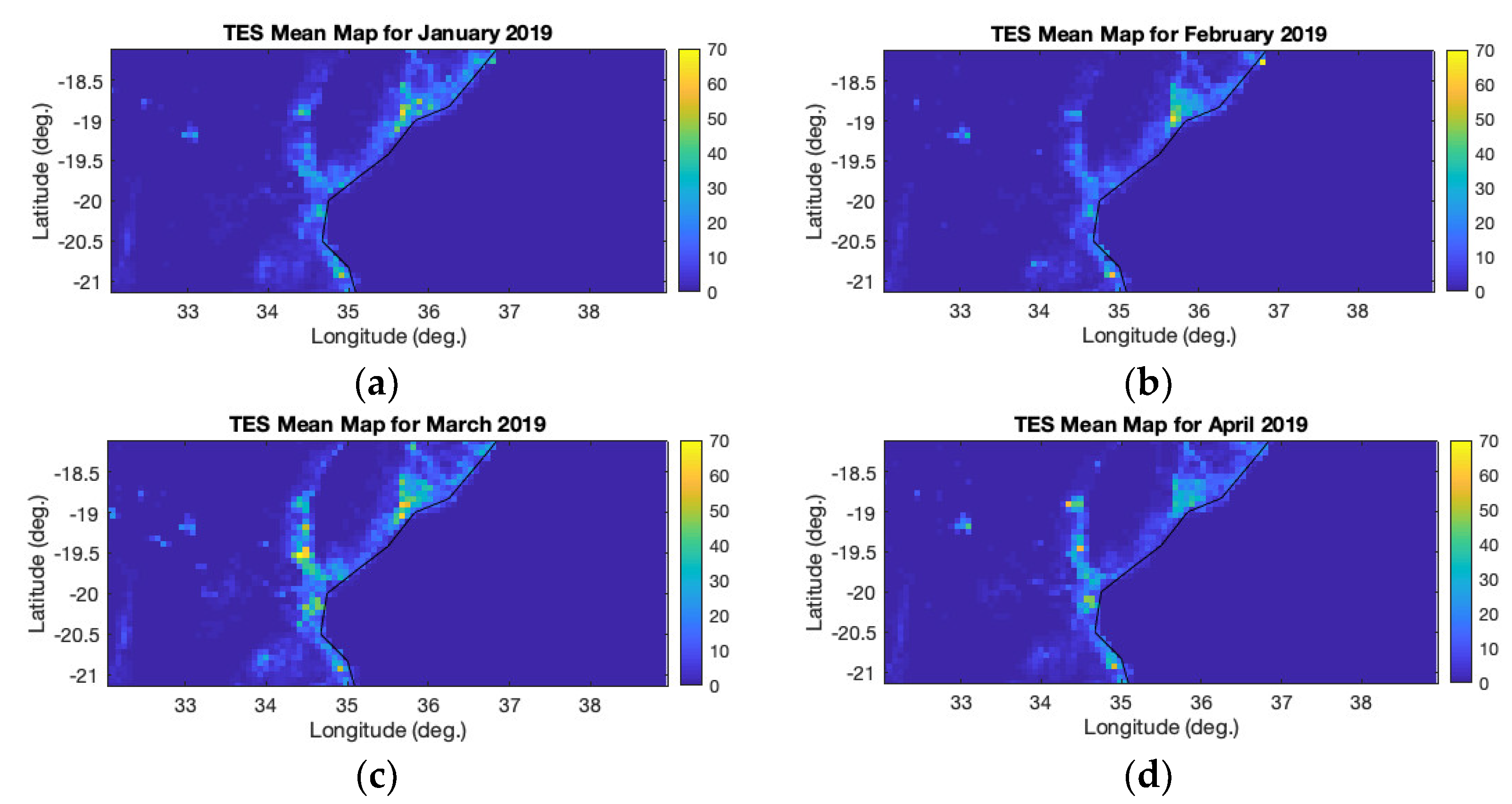
  • The trailing-edge slope (TES), which describes the shape of the reflectivity DDM and is computed as the slope to the right of the maximum value of the reflectivity DDM integrated in the Doppler domain (referred to as Integrated Doppler Waveform (IDW) or simply delay-waveform in the literature).
TES observable is selected as primary indicator, instead of the peak value alone, because the averaging is limited to 1 day of measurements over a small area, where no more than four observations for the same pixels are expected. Errors on the computed signal power become more relevant when averaging is not enough to produce a statistically significant data ensemble. TES is a more robust observable since it is related to the shape of the measurements: the scattering of the signal from inundated surfaces is significantly different from that of non-inundated surfaces and the shape is evident into the measurements, becoming steeper for inundated surfaces. In other words, the TES observable is linked to the nature of the scattering, coherent or incoherent, and it is less affected by small calibration effects. In terms of flood detectability, using an observable linked to the nature of the scattering will result in more positive detections (less probability of error) and therefore will result in a better capability to detect short duration floods, which occupy a small area within the CYGNSS footprint and need to be detected in a single pass of the satellites. Figure 1 shows an example of the waveforms measured under different flood conditions.
In Figure 1, red and green dotted curves represent the scattering from non-inundated surface conditions, while blue represents inundated surface conditions. As it can be seen the slope of the dark blue line is steeper if compared to both the red and the green. Red and green waveforms do not show strong differences in slope but green shows an increased power close to that of the blue waveform. This could lead to classification errors if the algorithm was based on peak information alone. The increase in power is not necessarily related to small calibration issues or noise, rather it may be the result of the inhomogeneity of the observed surfaces. In order to detect flooding of surfaces, it is necessary to have an observable that reflects the variability of the scene. In other words, the probability of positive detections increases if the distinctive nature of the scattering from standing water is captured in the observable. The particularity of the floods affecting the agricultural-urban interface is that they happen in a matter of 6 h and last 2 to 7 days, therefore, we cannot integrate data over several days. To detect those, the selection of the observables is key and adds more challenging requirements than the sensitivity provided by peak reflectivity alone.
Within these constraints, we have developed an algorithm that includes both peak reflectivity and TES observables by pre-classifying the pixels of the scene according to their statistical properties. Our flood product is able to comply with another of the requirements identified by the translator in which the landscape characteristics must be incorporated into the signal processing to better interpret the bistatic radar returns, eliminating the variability of the scene.

3.2.2. Considerations and Steps of the Classification Algorithm

Various assumptions and considerations were adopted leading to the algorithm being summarized as:
  • A gridding strategy is designed where each measurement is mapped onto the surface with its particular spatial resolution and then re-gridded into a grid cell of 3 km × 3 km, averaging overlapped areas within the same grid pixel.
  • CYGNSS data is averaged at 1 s incoherent time, as the new 0.5 s data was not yet available.
  • Each 3 km × 3 km pixel within the area under observation is considered independent.
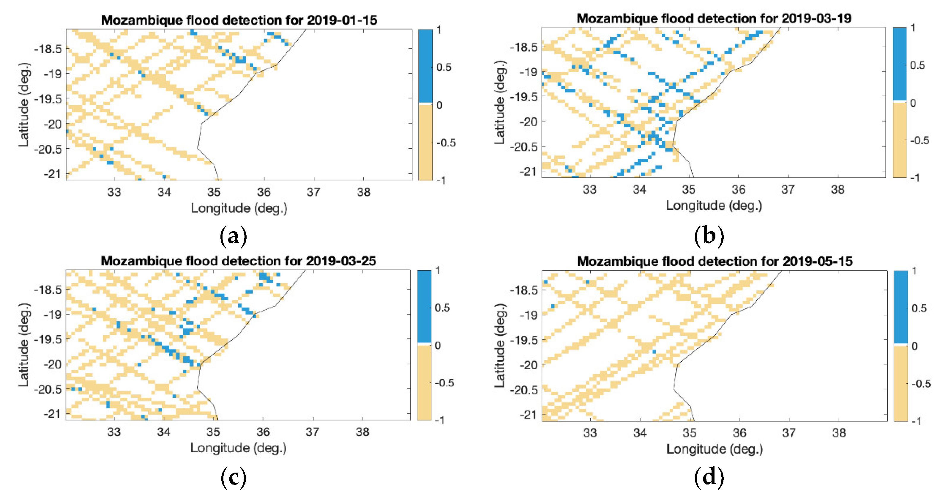
  • A 1 or 0 value is assigned to each pixel, being 1 = flooded and 0 = non-flooded.
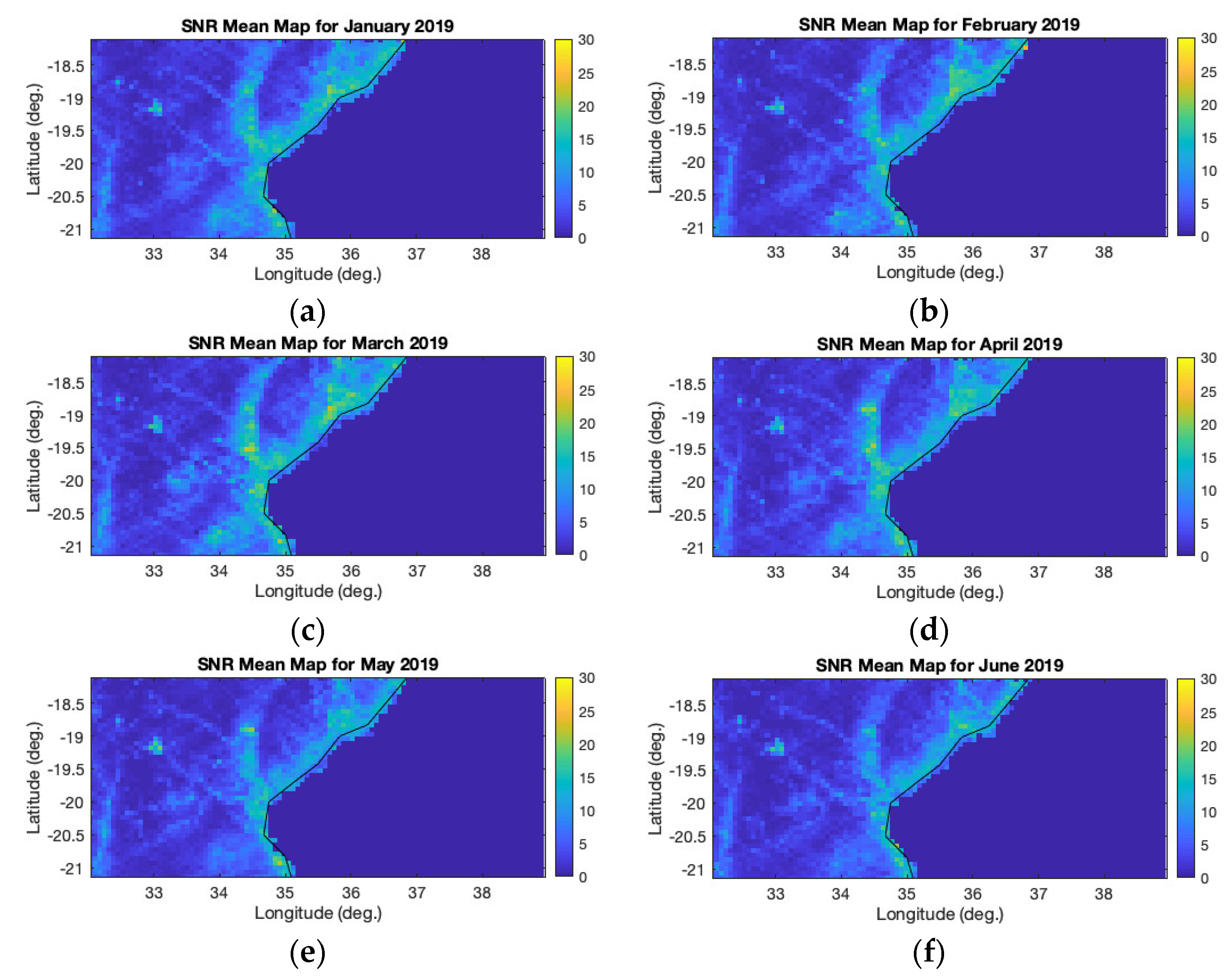
  • The best indicator is assumed to be the shape of the waveform, as discussed in Section 3.2.1, but still signal strength is used in combination. The selected observables are therefore TES and the peak SNR. When an SNR increase is observed with respect to previous measurements over the same area, it is indicative of the potential presence of standing water. Therefore, as long as peak SNR is referenced to the previous state, it will remain a good contributor to flooding detection. Steeper (increased) TES indicates an increased likelihood of standing water, and thus being indicative of flooding. Measurements coming from an area producing increased coherent scattering will potentially contain scattering signatures of the standing water. This observable also becomes stronger when referenced to values of the same area at previous instants of time.
  • SNR is calibrated using Equation (2). TES is produced from non-normalized waveforms considering the power increase along with the slope. We discarded normalization to avoid equalizing the inhomogeneity of the scene.
  • On a daily basis, 2-D maps in latitude and longitude coordinates of SNR and TES values are created for the area under study.
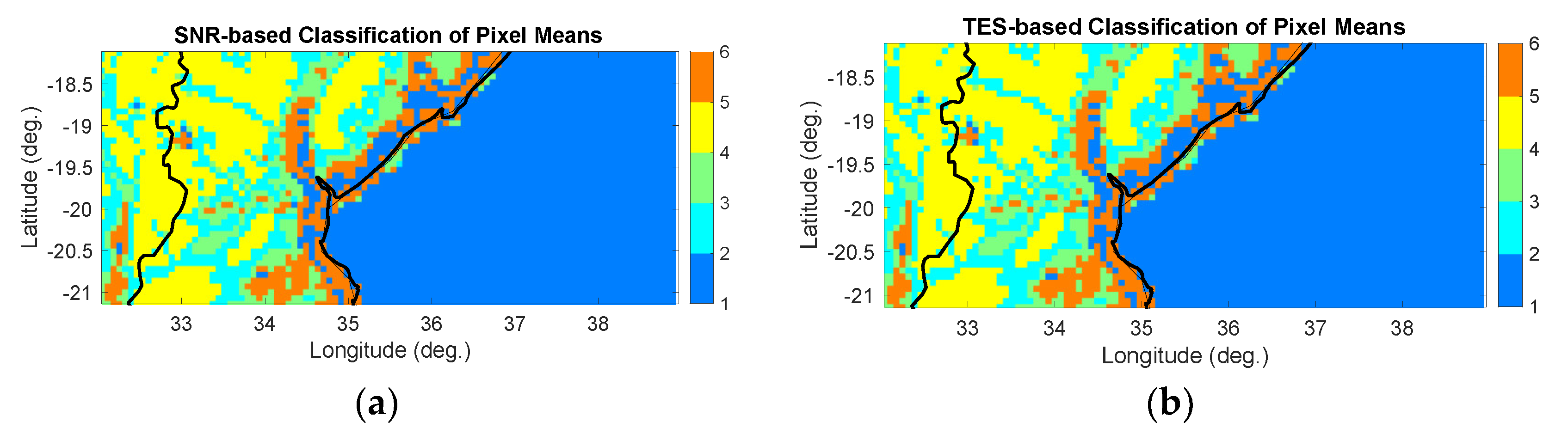
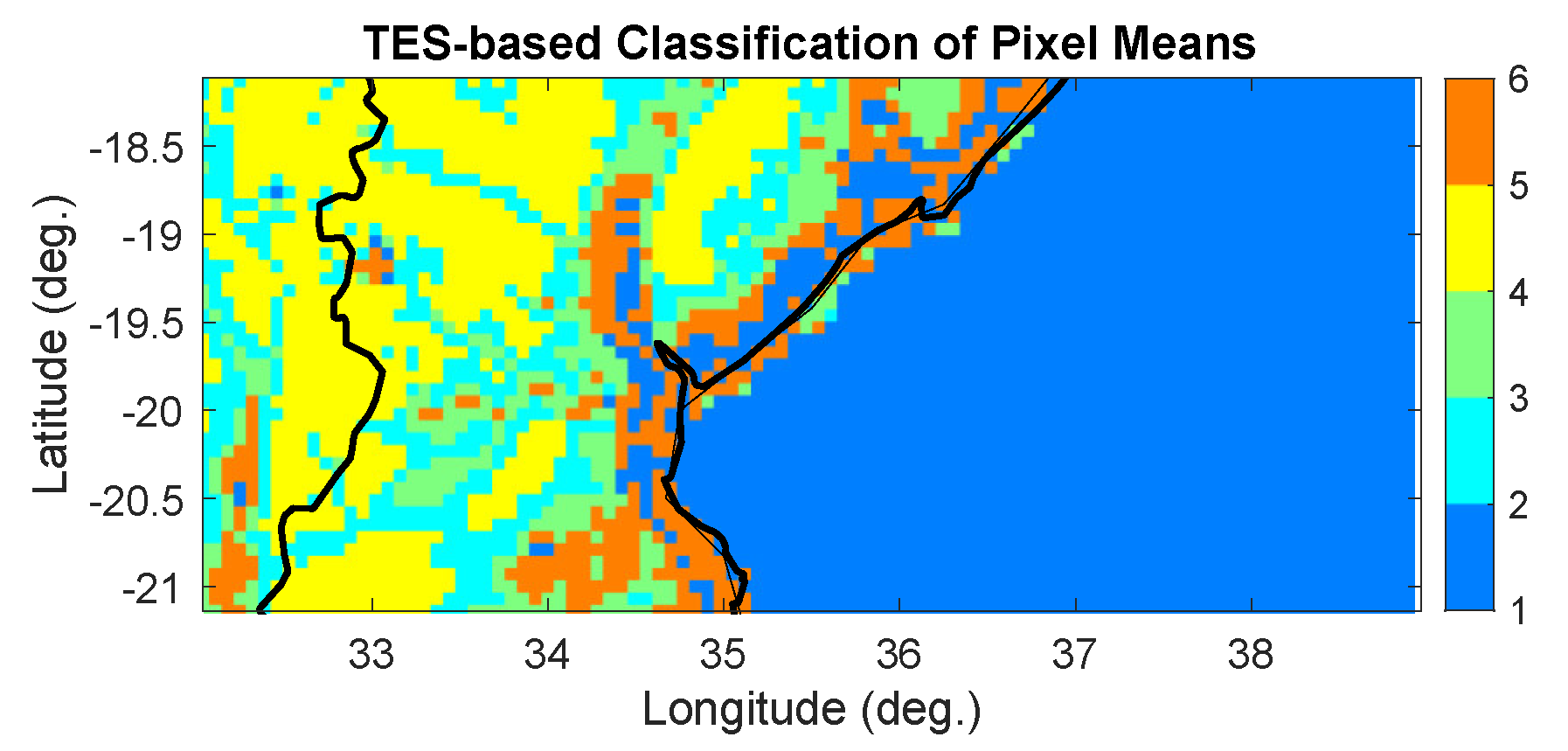
  • The 2-D SNR and 2-D TES maps in latitude and longitude coordinates are then analyzed during a whole year to classify the variety of pixels involved in the scene. For this, we use a k-means algorithm [51] that takes in the pixel’s values of the area under study for one whole year and classifies them. The selected number of classes is 6.
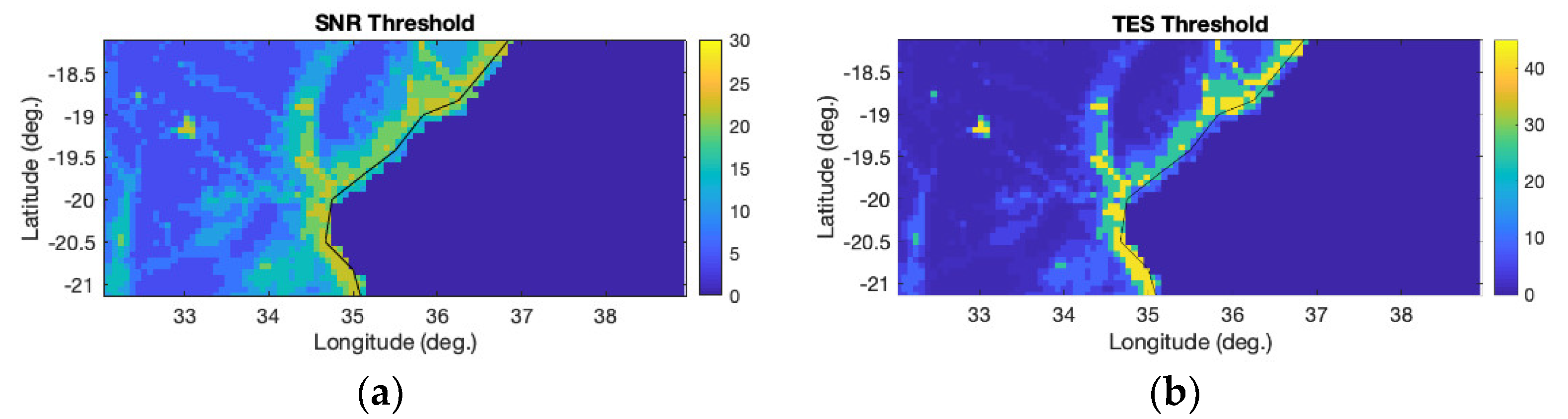
  • For each class we compute the mean and the standard deviation and set a threshold, computed as the mean plus two sigma, 2-D threshold maps for both SNR and TES variables. This step provides reference values to inform decisions on whether peak SNR increase or TES steepness originates from the presence of standing water.
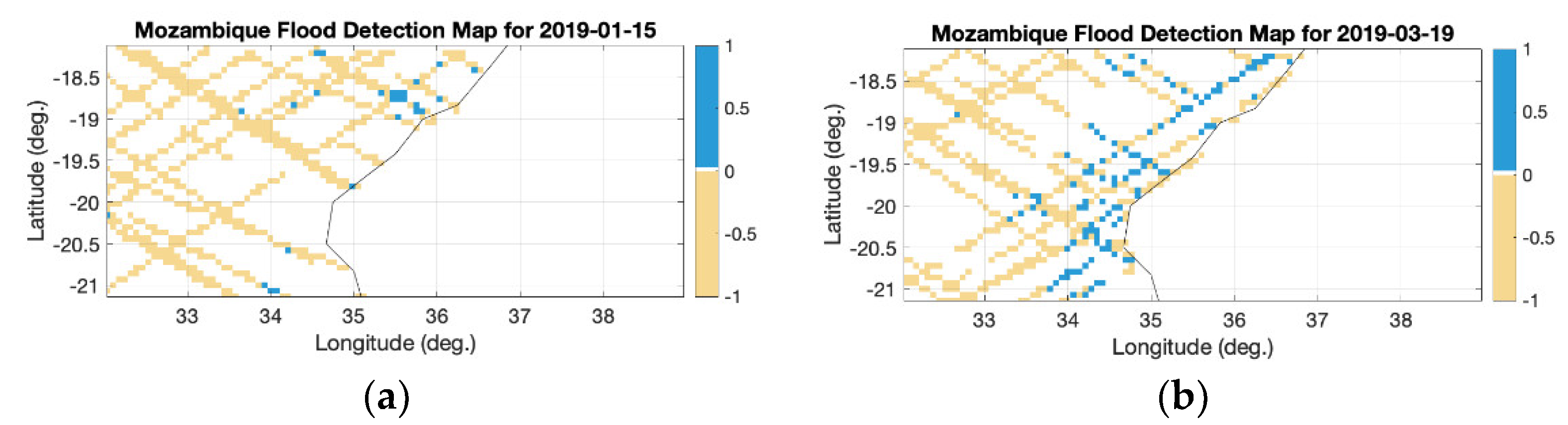
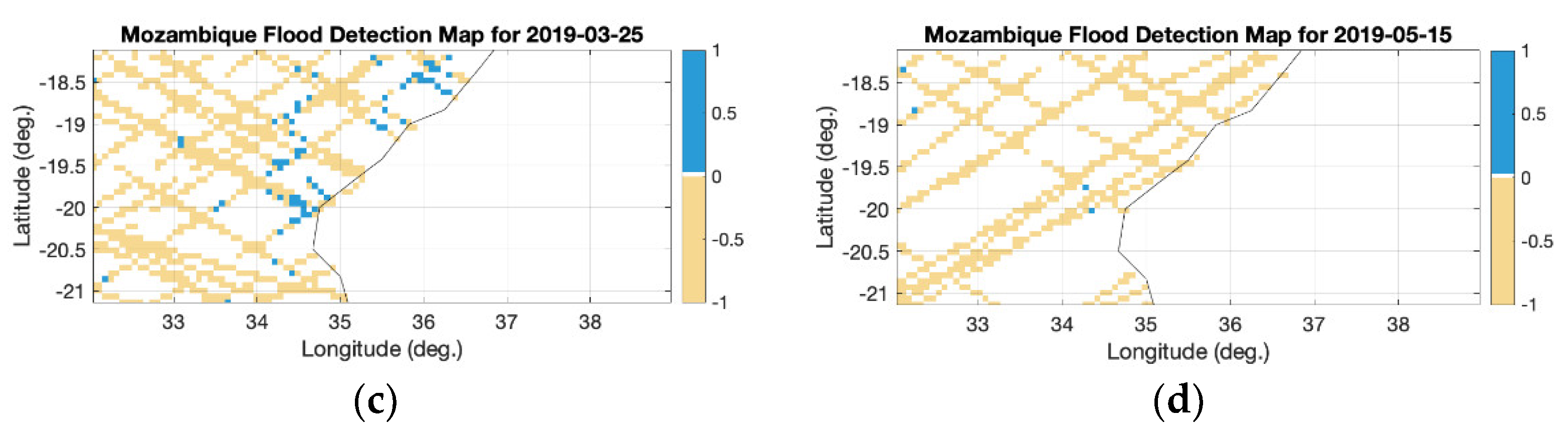
  • The 2-D SNR and 2-D TES maps are then subtracted from the corresponding 2-D threshold maps. Positive values are assigned to flooded pixels and negative values are assigned to non-flooded pixels, generating 2-D maps in latitude and longitude coordinates of flooded and non-flooded pixels.
Following the steps described from (1) to (10), 2-D TES and 2-D SNR maps are created for the areas under study, covering a whole year. GNSS-R measurements from CYGNSS have the ability to not only detect short-duration and localized floods but also monitor the soil conditions before and after, until the soil conditions are back to their original state (before the floods occurred). Further, beyond the scope of this work, the seasonality of soil conditions requires an annual assessment of what the baseline signals for inundation are in some areas, thus enabling the possibility to find flood risk indicators and flood impact indicators [55]. Additionally, roughness maps, land type, and vegetation information can be added as ancillary data to correct the variability in CYGNSS signals, together with SMAP soil moisture information, TRRM rainfall information, and topographic information. Doing so allows for potential added value to understand which soil conditions are more likely to cause flooding than others. Other studies, such as [53] for wetlands detection or [56] for dew distribution analysis, included different methods than the one here presented. For example, in the case of [53], a potential flooded wetland area mask was created based on the elevation difference between a digital elevation model (DEM) pixel and the nearest pixel that is part of the drainage network. In [56], satellite data was compared with meteorological data for precipitation, evaporation, and air temperature, and a very precise grid of 1 × 1° of longitude and latitude was created for dew distribution.

3.2.3. The Flood Classification Algorithm Main Element: K-Means Clustering

The classification algorithm is built around the exploration of both the SNR and TES observables’ samples for the whole observational period. The data analyzed is heterogenous and contains scattering variability due to the multiple sources within the scene. The main goal is to classify pixels into flooded/non-flooded conditions. The inundation signature on the shape of the waveform is strong enough to be able to be separated from any other source of variability. We employ a k-means clustering [51] strategy in order to divide our samples into six groups of samples whose mean represents the properties of each pixel within the scene. Pixels within each class are then analyzed in terms of mean value and standard deviation, which will be used to set the thresholds for each class. Both SNR and TES observable maps are then analyzed against the threshold maps and the pixels are classified into non-inundated/inundated. We have applied the k-means algorithm individually to pixels that share the same statistical properties, obtaining a map of thresholds rather than a unique threshold describing the whole area.
Therefore, the core of the classification algorithm is the k-means clustering [51] of the SNR and TES samples for each pixel using the data from the whole year 2019, which allows the identification of the statistical properties of each pixel and its classification into one of the six classes. K-means clustering, also known as Lloyd’s algorithm, is an iterative, data-partitioning algorithm that assigns the vector of observations to the number of indicated clusters, with each cluster defined by a centroid. We provided a total of two clusters since we aimed to classify the samples into two groups with dominant characteristics: inundated and non-inundated pixels. This algorithm: (1) selects k = 6 centroids, randomly; (2) finds the distances of each observation to the selected centroids; (3) assigns each sample to one of the centroids; (4) computes the average of the observations in each cluster to obtain k = 6 new centroid locations; and (5) re-iterates from steps 2 to 4 until cluster assignments do not vary.
An example of this can be seen in Figure 2, for Mozambique during the year 2019. Mozambique is one of the study cases selected that will be described in Section 3.3. Once pixels are separated into classes, we analyze them independently, computing the mean value ( μ ) and standard deviation ( σ ) of the samples. We found that the optimal threshold (Th) that best separates the samples within each class is T h = μ + 2 σ for each corresponding class μ and σ values.
Classifying individual pixels according to their statistical properties reduces variability in the scenes and avoids confusing SNR variations originating from the natural scattering of heterogeneous land scenarios with changes in flooding conditions. This initial pixel class characterization is recommended in order to treat independent pixels with different initial states, or background values. This initial step is key as an arid area will present a threshold much lower than a moist area around a delta, for example. Once these thresholds are obtained, the SNR and TES values are analyzed on a daily basis, classifying the pixels into inundated versus non-inundated based on the typical mean and standard deviations of the pixels of the same class. From there, 2D flooding maps are generated. If the assumption is right and the main characteristic of the dataset is dominated by inundation conditions, the algorithm is expected to classify the pixels as inundated just for the period the flooding occurred, including recovery time, i.e., the period of time from initial flooding until return to normal. Next, we show the methodology applied to two case studies, as summarized in Table 3.

3.3. Case Study 1: Results for 2019 Mozambique Floods

3.3.1. Background

In 2019, two tropical cyclones impacted Mozambique in the course of a few weeks, with impacts demanding a humanitarian response (Figure 3). Cyclone Idai made landfall near Beira city on 14 March 2019 with Cyclone Kenneth following soon after when making landfall near Pemba on 25 April 2019.
Cyclone Idai led to hundreds of deaths and massive destruction of property and crops, however, it was the extreme rainfall driven floods, rather than the wind, which led to the majority of impact [8,57]. Less than six weeks later, on April 25, Cyclone Kenneth impacted northern Mozambique, approximately 600 miles north of Idai’s primary impact zone. While the close succession of the events led to amplified and compounding impacts, forecasts were available each for the track, rainfall, flooding, and winds. Additionally, longer timescale forecasts on the seasonal scale had been indicating a heightened risk of El Niño developing. Under these premises, through January–February there were decisions made to anticipate drought in Southern Africa. In early March, Cyclone Idai was forecast, presenting the need to react by taking anticipatory actions to decrease the risk of flood and wind impact, rather than drought—leading to complications in prioritizing what types of actions were halted, revised, and commenced. Idai, a wetter storm than expected had far-reaching impacts inland to Malawi and Zimbabwe, areas that are less prepared to anticipate impact from tropical cyclones.
While flood maps were produced for this event, such as those derived from Sentinel-2 and ALOS-2 [58,59], our method would have provided an additional approach which could have led to improved decision-making during response and recovery activities.

3.3.2. Data Analysis

To assess the ability of our method to detect flooding during this event, we focus on a daily time step. For example, one of the inputs is the monthly means of TES and SNR, which are computed from the daily maps for each month over the year to see the evolution of soils. Figure 4 shows the monthly means from January to June 2019 for the TES observable.
Through the TES monthly means we can assess the status of the soil for that particular month. Indicators that the soil is starting to become moister would appear as increased TES mean values. This provides an indicator of flooding but is also critical to assess the potential impact of cyclone events. For our case study, this can be seen in Figure 4c, the monthly TES means for March were increased as expected due to the flooding that occurred and that extended into April. Consequently, the monthly means for May and June returned back to initial levels, like the ones in January, indicating the recovery of the soil. Basically, the six maps in Figure 4 explain the flooding event from its origin to its recovery. Figure 5 shows the monthly means of SNR.
Similarly, through the SNR monthly means, we can assess the status of the soil for that particular month. The TES value is expected to be a better flooding indicator since it is related to the shape of the measurements, i.e., the scattering of the signal from inundated surfaces is significantly different from that of non-inundated surfaces and the shape is evident in the measurements. This may explain why SNR does not capture little soil moisture changes, but the monthly SNR means for March were still able to capture the expected increase in surface reflectivity due to the flooding, and it can also be seen how it extends to April. May and June monthly SNR means return back to initial levels, like the ones in January and February, indicating the recovery of the soil. Equally daily SNR and TES maps can be produced over time frames of interest. For example, in Figure 6 we show the TES and SNR daily values for 18 March 2019 to 20 March 2019, providing a more detailed insight and a more focused time scale to analyze a particular event.
The algorithm will then proceed by analyzing a certain amount of data. For this case study, we used a whole year, but it would be possible to use a shorter time as long as the seasonality and statistical properties of the scenes are captured. The amount of data used prior to the event for the analysis allows the classification of the pixels according to their statistical properties (Figure 7).
As it can be seen in Figure 7, both observables provide consistent results, which makes the approach robust since the k-means algorithm [51] employs the statistical properties of the surfaces under consideration. Indeed, the k-means algorithm we have developed represents a new methodology for land classification applications. It is possible that if we chose an elevated number of classes, we would observe more variability as the SNR is more sensitive to differences in reflectivity. Note that this information can also be key in learning more about the surface properties and how, for example, soil moisture tends to accumulate in some areas more than others. Then, the pixels in each class are analyzed in terms of mean and std and the following threshold maps are obtained for each class, Figure 8.
Threshold maps are then used to assign each pixel a binary value of flooded or non-flooded for specific days. Figure 9 and Figure 10 show the flooding maps obtained for 15 January 2019, 19 March 2019, 25 March 2019 and 15 May 2019, using SNR and TES information respectively.
According to the translator specifications, another relevant output that can be provided to decision-makers is the temporal evolution of the number of observed inundated pixels. Figure 11 shows the results for both SNR and TES observables.
Figure 11 shows the % of inundated pixels, per day, normalized to the total number of pixels measured within the area under study in order to account for the difference in coverage from one day to the other. As it can be seen, plots in Figure 11a,b show similar behavior, although SNR observable displays more variability on the number of pixels classified as flooded. As the algorithm is avoiding most of the confusion caused by the variability of the scenes, ensuring pixels are classified within the same statistical properties, the flooding detected by SNR brings added information to the one detected by TES observable. In fact, looking at the temporal series obtained for the SNR observable we can see a double bounce between 14 March 2019 and 30 April 2019, which corresponds to the respective impacts of Cyclone Idai on 14 March 2019 and Cyclone Kenneth on 25 April 2019. Those are also apparent on the TES-based results, but much smoother since the roughness of the waters would reduce the steepness of the TES observable. In conclusion, the combination of both observables is key to fully understanding the events. Figure 11a,b provides insight into the recovery time of the soils. Similar images can be produced at the pixel level or focused in certain areas to better understand the recovery times of the whole area under study, producing maps of the estimated time of recovery for each pixel. Rainfall (Figure 11c) has a higher degree of correlation with SNR results in Figure 11a which indicates that the SNR observable is more affected by the moisture of the soil being altered by precipitation than TES is.

3.4. Case Study 2: The US Midwest Spring Floods—Northeast Arkansas

3.4.1. Background

In this case example, we perform the analysis of the inundation dynamics caused by the Midwest spring floods over north-east (NE) Arkansas in 2017. This event is different from the Mozambique case, as floods were caused by recurrent thunderstorms rather than tropical cyclone related rainfall and subsequent riverine flooding. The USGS river status maps [61] reported rivers above flood stage in NE Arkansas between 28 April 2017 and 8 May 2017 coincident with the Midwest spring floods event. Therefore, the spring floods in NE Arkansas, driven by heavy rainfall, were the result of both riverine and pluvial floods together with urban floods (Figure 12). From the USGS river level reports (Figure 12d), the area affected within CYGNSS coverage (from 37 S to 37 N in latitude) is north-east (NE) Arkansas. Note that latitude 37 N is just over Arkansas’ northern state line. A box corresponding to 34.88 deg. and 36.42 deg. latitude and −91.69 deg. and −90.36 deg. longitude was selected for our analysis, encompassing the areas of Newport, Jonesboro, Paragould, Pocahontas, and Walnut Ridge.

3.4.2. Data Analysis

We applied our algorithm and obtained the flood classification results in Figure 13, which are based on TES observable, i.e., the same result as for Figure 10 in the Mozambique case.
Flood detection maps corresponding to days during the Midwest spring floods, including riverine, pluvial, and urban types of floods, i.e., 30 April, 1 May, 4 May, and 5 May 2017, show an elevated number of flooding detections (the blue pixels in Figure 13). For other days selected randomly before the storm, 20 April 2017, and after the storm, 10 August 2017, the classification algorithm did not detect flooded pixels (pale orange). There are some false positives that could be caused by either the presence of a river in the CYGNSS footprint or classification errors. For Figure 13c–f, the number of flooded pixels increases in areas where river levels above flood stage were reported by the USGS, Figure 12d, corresponding to areas around the Current River, Black River, and the White River from Pocahontas–Jonesboro–Paragould southwards toward Little Rock in Pulaski County and Lonoke County.
Next, we explore the capability of the method to define the recovery period of flooding events, as we did for the Mozambique case. To do so, we performed an analysis of the number of flooding pixels per day, normalized to the total number of pixels measured within the area under study in order to account for the difference in coverage from one day to the other. In addition, we inspected the correlation with the rain events that happened in the area under observation (Figure 14).
Figure 14a shows a daily analysis of the number of flooded pixels with respect to the number of measured pixels within the area under study. Figure 14a includes data whose observations for one day cover in mean 40% of the total area under study. Looking at Figure 14a, it is clear that during the Midwest spring floods period that affected NE Arkansas, the number of detected flooded pixels increased dramatically, starting 28 April and with the peak on 30 April 2017. Figure 14a also shows the recovery period, i.e., the period of time that elapses until soil conditions are back to their initial state (before flooding happened). Additional rain events during the recovery time may aggravate the soil conditions and therefore will cause longer recovery times. Therefore, the recovery time depends on initial soil conditions as well as recursive rain events during the recovery period.
Precipitation data in Figure 14b corresponds to the daily accumulated precipitation product generated from TRMM_3B42RT_daily product [60]. The values provided in the TRMM dataset correspond to the summation of hourly valid retrievals in each of its grid cells for one day, and they are provided in mm units. Soil conditions are likely to be saturated after recent flooding, and a new storm can aggravate the conditions of the soil and cause recurrent floods, or areas not being able to absorb the falling rain. The flooding event was caused by a series of convective storms with over 125 mm on 30 April. A later storm, on 27 May 2017, added 80 mm precipitation. However, the second storm caused the soil conditions to stay saturated until 10 June 2017, when recovery towards normal conditions began, a total of 68 days.

3.4.3. Validation of Floods in Arkansas

The Global Flood Monitoring System (GFMS, [16,63,64]) can be used as a source to validate our methods. GFMS is a NASA-funded experimental system using real-time TRMM Multi-satellite Precipitation Analysis (TMPA) and Global Precipitation Measurement (GPM) Integrated Multi-Satellite Retrievals for GPM (IMERG) precipitation information [65] as input to a quasi-glob–l (50° N–50° S) hydrological runoff and routing model. Flood detection/intensity estimates are based on 13 years of retrospective model runs with TMPA input, with flood thresholds derived for each grid location using surface water storage statistics (95th percentile plus parameters related to basin hydrologic characteristics). This product is therefore not based on actual measurements of the surface conditions, but it provides an assessment of probability occurrence based on 13 years of data. To compare the assessments from our flood product, we have looked into a dataset from the GFMS dataset for the same area and timeframe of the US Midwest spring floods in NE Arkansas. This case study represents a more localized area affected by a type of flood more challenging to detect from space, than those of hurricanes. We have obtained the validation data from the GFMS website at [64]. In Figure 15 we display the flooding maps produced by the GFMS, for the same days displayed in Figure 13.
Flooded pixels (depth above threshold in mm) are detected in maps Figure 15c to Figure 15f, (30 April, 1 May, 4 May, and 5 May) as our k-means based GNSS-R classification estimated. The results obtained with our GNSS-R classification algorithms (Figure 15), i.e., surface measurement-based method, are compared to the results of the GFMS flooding product (Figure 15), i.e., memory model-based with precipitation information. A total of 93.7% of the pixels classified by our algorithm as flooded were also identified as flooded by the GFMS product (6.3% discrepancy). Only 68.46% of the pixels classified as non-flooded were also identified as non-flooded by the GFMS product (a discrepancy of 31.54% between the two products). This 31.54% discrepancy between the GNSS-R non-flooded classifications and the flooded GFMS product has different origins (Table 4).
The highest values of discrepancy are found in areas where the depth above threshold was between 0.001 and 10 mm, which indicates shallow inundation. Looking at Figure 15b–f it can be seen from where the discrepancy source originated. The green area showing shallow inundation 0.001 mm to 10 mm was not reported by the NWS or the USGS sources at any moment during the Midwest spring floods, therefore implying green areas in Figure 15 overestimate the amount of flooding. Note that the GFMS maps are based on model predictions mixed with actual precipitation and therefore do not represent an actual measurement of the surface conditions. It is also possible that the TES threshold selected by our k-means clustering estimator is not accurate enough, as our k-means classificatory and threshold estimator is designed to account for the differences originating in the landscape at a pixel level. GFMS product is used because it covers the whole duration of the flooding event, as opposed to SAR-derived products such as the one obtained from Sentinel satellites, with a cadency of 6 days for the 2017 Midwest spring flood event. GFMS products allow therefore a day-to-day comparison with our product estimations.

4. The Humanitarian Component

4.1. The Translator Role

The translator role, in this context, allows for the opportunity for the decision-maker to provide input to the scientist to allow for a more efficient and effective data development and dissemination process, [10,66,67]. For example, the scientist will likely have a perception of what types of data, and in what form, would be useful for decision-makers. However, this perception could be incorrect, leading to a situation where data and derived products lead to less efficient and more complex decision-making processes [68]. Spatial and temporal scales are elements whereby translators can be aware of the limitations and opportunities presented by the data, interacting with the decision-makers from a trusted position [69]. The translator would approach the discussions with decision-makers from a perspective whereby they can assess qualitatively the limitations and constraints of the decision-making context, and repackage that information into data points (such as minimum standards for lead time, appropriate temporal range, and acceptable spatial scale) to the scientists. This could be critical in terms of efficiency of the scientists disseminating data as even the reduction of one iteration could save days of time which, in a humanitarian emergency, can lead to a significant saving of life, livelihoods, and property [70,71].

4.2. The Decision-Maker Role

The decision-maker may have limited connection with the data scientist writing the codes, however some interaction, if and when facilitated by the translator, could be beneficial, especially in terms of building trust between the three actors, which could potentially lead to increased perceived ‘trustworthiness’ of the data. It is important to avoid the creation of a hierarchy of importance around the three actors. One way to avoid doing this could be to elevate the ‘data’ generated by the decision-maker to the same level of value as the data generated by the data scientist. For example, the traditional framing of data produced by a scientist to allow for improved decision making can be reversed, in framing the data collected by the decision-maker, such as the quantitative data of the amount of time it takes to execute an action, as also a data point and as allowing for the scientists’ data outputs to reach a higher level of quality, relevance and trust [72,73]. This framing should be employed from the earliest possible stages of engagement/projects possible.

5. Discussion

5.1. On the Usefulness of Signals-of-Opportunity

The results shown in this study demonstrate the great potential of signals-of-opportunity to detect flooding at the human-natural interface. One challenge with the detection of floods driven by heavy precipitation leading to localized flooding is cloud cover. Having a source of signals at L-band, that can see through cloud cover and day/night conditions, makes the measurements ideal. We have demonstrated that CYGNSS offers measurements from minutes to hours apart of the same area, evidencing that both floods and flash floods at the human-natural interface can be detected and monitored in some contexts. Particular flash floods could still be missed if the events occur in the order of a few kilometers or sub-kilometers with a rapid onset and short duration. In addition to the L-band signals used in this study, it would add value to incorporate other measurements, such as SMAP-R, when available. Also, it would be beneficial to incorporate P-band measurements from other sources of opportunity. For example, if a constellation of satellites was able to provide combined measurements at L-band and P-band from multiple sources of opportunity (i.e., GNSS for L-band and Mobile Use Objective System for P-band [74,75]) the amount of information collected would very much benefit the sampling repeat and the coverage over more localized areas. We note a direct correlation between the number of signals collected and the increased accuracy of flood detection and therefore advocate for increased attention to the development of missions that will produce this data. With the increased accuracy, especially related to events occurring on very limited spatiotemporal scales, the disaster risk community will likely have an increased understanding of opportunities to develop flash flood-specific early warning early action strategies. Flash floods that exist on extremely small spatial and temporal scales would then be possible to assess in near-real-time. In addition, the combined L-band/P-band information would represent complementary data through the different penetration depths, increasing the understanding of why certain areas are at higher flood risk than others as well as the current conditions of soil layers.

5.2. On the Benefit of Multi-Sensor Information

Adding CYGNSS information to model-based predictions could improve accuracy. In addition, signals-of-opportunity could be combined with other sensors such as radiometers and synthetic aperture radars (SAR) or radars to obtain optimum information and produce an enhanced product. Measurements from the Sentinel-1A C-band SAR or the phased array type L-band SAR 2 (PALSAR-2) would benefit from GNSS-R measurements as a complement to fill in the gaps due to the measurement’s cadency. Also, the multispectral imagery from MODIS or Sentinel-2A/B, limited by cloud and dust in the atmosphere and day/night conditions, would be greatly enhanced by CYGNSS measurements at L-band—not affected by any type of weather or day/night condition. For example, for the case under study, the 2019 Mozambique floods, GNSS-R could help fill in the gap between Sentinel available data, and generate a combined product with a higher revisit time. The inclusion of an L-band radiometer into the mix brings added information on the soil moisture conditions and even though current missions, such as SMAP offer very coarse information on the order of 36 km with an enhanced product at 9 km, the information is very relevant to understand the condition of the soils pre-, during and post-flood event. Combined with CYGNSS information alone, or with the merging of a SAR, CYGNSS and multispectral information, a product as SMAP soil moisture is key. The addition of ancillary information such as precipitation from TRMM, as well as roughness and digital elevation models would create a very comprehensive pool of information and would allow for the development of an advanced algorithm leading the way to a flood risk assessment product.

5.3. On the Co-Development of Comprehensive Flood Risk Products

This manuscript has shown an initial approach designed to bring together technological and scientific capabilities and humanitarian specific needs with the goal of creating a flood product. The ultimate goal of the research we are conducting and the path we will follow is to develop a flood risk product that is meaningful to decision-makers and can therefore have a real impact on the disaster management of underserved communities and areas prone to flooding. The described collaboration between scientists, translators, and agents from local entities will bring novelty to this research field, as flood product co-development with these actors has been extremely limited.
Current flood preparedness and response capabilities include satellite observations, data systems, and modelling capabilities through a number of operational products shown in the introduction (i.e., GFMS, NRT MODIS Flood Mapping, or ARIA). In terms of technological and scientific capabilities, those developments lack the combined high spatial resolution and temporal repeat of the reflectometry data from the CYGNSS mission. CYGNSS data provides insight into the flooding events as no other sensor or mission can see them, and employing this data results in suitable flood products to characterize rapid events.
In terms of humanitarian and flood risk reduction capabilities more broadly, no has been co-developed between an academic institution, active in addressing humanitarian needs, and a research facility with long expertise in Earth science data, and in that sense, this type of collaboration will pioneer these new initiatives. Our presented work enhances ongoing collaboration where we have demonstrated an original methodology that uses CYGNSS mission bistatic radar measurements and an artificial intelligence classification algorithm based on statistical properties of the land pixels through a k-means clustering strategy to detect and monitor flooding events, as well as to characterize the land surface prior to and post flooding events.

6. Conclusions

This manuscript helps define the roles required in the development of a technological, scientific, and humanitarian flood product: scientist/technologist, translator, and decision-maker.
On the technological/scientific side, we have provided an original methodology to detect and monitor flooding events as well as to characterize the land surface prior and post flooding events, using CYGNSS mission bistatic radar measurements and an artificial intelligence classification algorithm based on the statical properties of the land pixels. We employ a k-means clustering [51] strategy, dividing our samples into six groups of samples whose mean represents the properties of each pixel within the scene. Pixels within each class are then analyzed in terms of mean value and standard deviation, which will be used to set the thresholds for each class. Both GNSS-R SNR and TES observable maps are then analyzed against the threshold maps and the pixels are classified into non-inundated/inundated. In the second stage, therefore, we re-apply the k-means algorithm individually to pixels that share the same statistical properties, obtaining a map of thresholds (uniquely defined for each pixel in the scene).
We have demonstrated that the CYGNSS constellation has the very unique capability to capture flood events over considerable areas, such as the 2019 Mozambique floods, but also smaller flood events, such as the inundation in Arkansas during the 2017 U.S. Midwest spring floods. We have proved the capability to measure at a daily rate, which is key to capturing flash flood events. We have found that by employing the novel methodology, the highest values of discrepancy are found in areas where the depth above threshold was between 0.001 and 10 mm, which indicates shallow inundation. For depts over 10 mm, the discrepancy is always below 4.5%. Also, we have shown that CYGNSS data is not only sensitive to flood state but also to varying soil moisture conditions, proving that the methodology used is also a valuable asset to track soil state until conditions are back to normal, therefore providing valuable information about the recovery of the affected areas.
Even though CYGNSS provides a very good temporal revisit of the areas, it is important to note once more that, ideally, a better spatial resolution in the order of meters is preferable. Next steps should be directed towards merging both optical imagery and synthetic aperture data with the CYGNSS dataset to be able to provide a substantial improvement in the spatial resolution for a better flood product.
On the translation side, we have established the actions and products that need to be generated in order to interface with the decision-maker. Also, we have identified some specific examples of decision-maker needs that have been presented in the form that a decision-maker understands, passed through the translator, and delivered to the technologist/scientist to incorporate or to help shape the original maps. The approximation to the problem developed in this study brings novelty to the standard applications previously developed with CYGNSS data by incorporating the humanitarian component through the translator component to be able to develop a product tailored to the specific needs of the end-users.

Author Contributions

Conceptualization, N.R.-A. and A.K.; methodology, N.R.-A. and A.K.; software, N.R.-A.; validation, N.R.-A. and A.K.; formal analysis, N.R.-A.; investigation, N.R.-A. and A.K.; data curation, N.R.-A.; writing—original draft preparation, N.R.-A.; writing—review and editing, N.R.-A. and A.K.; visualization, N.R.-A.; funding acquisition, N.R.-A. and A.K. All authors have read and agreed to the published version of the manuscript.

Funding

This research was funded by Jet Propulsion Laboratory/California Institute of Technology through Engineering & Science directorate operations funds, under a Raise-the-Bar project, grant number OPO300-ESD OPERATIONS—RTB.33.UNIV. 20.02-IR—FLOOD DET. This project covered the funding required by N.R.-A. to conduct the investigation. In addition, this research was funded by NASA Grant #80NSSC18K0342: Towards a Global Flood & Flash Flood Early Warning Early Action System Driven by NASA Earth Observations, which covered A.K. to support the investigation.

Institutional Review Board Statement

Not applicable.

Informed Consent Statement

Not applicable.

Data Availability Statement

Publicly available datasets were analyzed in this study. We employed CYGNSS dataset that can be found at [76]. We also employed averaged daily rainfall obtained from the TRMM (TMPA-RT) Near Real-Time Precipitation L3 1 day 0.25 degrees × 0.25 degrees V7 (TRMM_3B42RT_daily) at GES DISC, through NASA Earth Data website at [77]. We have also employed Global Flood Monitoring System (GFMS) data available at [65].

Acknowledgments

This work was carried out at the Jet Propulsion Laboratory, California Institute of Technology, under a contract with the National Aeronautics and Space Administration © 2022 All rights reserved.

Conflicts of Interest

The authors declare no conflict of interest.

Appendix A

The following describes the general approach to map the DDM information to its native spatial resolution [44,45,46,47] as presented in [38]:
  • A power threshold is applied to the DDM in order to estimate the area from which the scattering signal is coming from. In order to set a threshold, most of the area representing the total power needs to be accounted for. We select a threshold that gathers the N% of the total power, N being an arbitrary number. According to the results in [34], a threshold of 80% is recommended.
  • Map the delay and Doppler values into the surface, drawing the iso-delay and Doppler lines. Both delay and Doppler provide the exact area of the scattering considered. For the sake of simplicity, we use the delay value alone, which translates to an ellipse in the surface. Therefore, the delay gathering 80% of the power is transformed into an ellipse of constant delay on the surface (iso-delay line). The size of the scattering area is set to the semi-major axis of the computed ellipse to represent the scattering area of that particular measurement. The summary table provided in [38] is annexed here in Appendix B, Table A1, for completeness.
  • The ellipse is centered in the specular point and is rotated to the scattering plane formed by the receiver and transmitter geometries, with the semi-major ellipse axis aligned with the scattering plane and the semi-minor axis perpendicular to it.
  • The ellipse is then elongated by the distance obtained by multiplying the integration time by the velocity of the satellite in the along-track direction.
  • The final elongated ellipse is mapped onto the surface with a fine enough grid that allows the delineation of the shape of an ellipse.
Steps 1 to 5 are repeated for all measurements.

Appendix B

A study performed in 2018 used SMAP-Reflectometry data to provide a table of spatial resolution of GNSS-R measurements, [38]. We make this table available here for completeness.
Table A1. Variable spatial resolution of GNSS-R measurements from SMAP-Reflectometer.
Scenario N = 80%N = 75%N = 70%N = 65%N = 60%
μ   k m σ   k m μ   k m σ   k m μ   k m σ   k m μ   k m σ   k m μ   k m σ   k m
Sea Ice2.80.92.40.82.10.61.80.31.80.25
Lake2.70.82.60.92.30.71.50.251.50.26
Wetland9.62.83.31.42.80.52.40.342.10.28
Arid Land13.35.86.44.25.32.64.92.34.32.4
Low Vegetation20.26.612.55.612.14.211.93.98.63.3
High Vegetation43.17.338.96.526.64.526.24.123.58.5
Ocean45.38.444.87.944.67.642.36.841.16.4
Values produced for ocean scenarios in [38] Table A1 are not applicable to CYGNSS because we observe the effect of the SMAP high gain antenna filtering the scattered signals into its main beam width of 40 km. The rest of the values presented in the table are expected to be in the same order. Particularly for wetlands, arid land, and low vegetation as in agricultural fields, the values are well characterized. High vegetation may be different as it gets closer to the SMAP antenna footprint.

Appendix C

CYGNSS data has been filtered using the quality flags shown in Table A2.
Table A2. CYGNSS L1 data quality flags used in this study, same as [43,54].
Quality FlagFlagged in Analysis
Poor Overall QualityNo
S Band Powered UpYes
Small Spacecraft Attitude ErrorNo
Large Spacecraft Attitude ErrorYes
Blackbody DDMYes
DDMI ReconfiguredYes
Space wire CRC InvalidYes
DDM is Test PattenYes
Channel IdleYes
Low Confidence DDM Noise FloorNo
SP Over LandNo
SP Very Near LandNo
SP Near LandNo
Large Step Noise FloorNo
Direct Signal in DDMYes
Low Confidence GPS EIRP EstimateYes
RFI DetectedYes
BRCS DDM SP Bin Delay ErrorNo
BRCS DDM SP Bin Doppler ErrorNo
Negative BRCS Value Used for NRBCSNo
GPS PVT SP3 ErrorNo
SP Non-Existent ErrorYes
BRCS LUT Range ErrorNo
Antenna Data LUT Range ErrorNo
Blackbody Framing ErrorYes
FSW Comp Shift ErrorNo

References

  1. Jonkman, S.N.; Vrijling, J.K. Loss of life due to floods. J. Flood Risk Manag. 2008, 1, 43–56. [Google Scholar] [CrossRef]
  2. Du, W.; FitzGerald, G.J.; Clark, M.; Hou, X.Y. Health impacts of floods. Prehospital Disaster Med. 2010, 25, 265–272. [Google Scholar] [CrossRef] [PubMed]
  3. Fiorillo, E.; Crisci, A.; Issa, H.; Maracchi, G.; Morabito, M.; Tarchiani, V. Recent changes of floods and related impacts in Niger based on the ANADIA Niger flood database. Climate 2018, 6, 59. [Google Scholar] [CrossRef] [Green Version]
  4. Morán-Tejeda, E.; Fassnacht, S.R.; Lorenzo-Lacruz, J.; López-Moreno, J.I.; García, C.; Alonso-González, E.; Collados-Lara, A.J. Hydro-meteorological characterization of major floods in Spanish mountain rivers. Water 2019, 11, 2641. [Google Scholar] [CrossRef] [Green Version]
  5. Demeritt, D.; Nobert, S.; Cloke, H.; Pappenberger, F. Challenges in communicating and using ensembles in operational flood forecasting. Meteorol. Appl. 2010, 17, 209–222. [Google Scholar] [CrossRef]
  6. Doswell, C.A.; Brooks, H.E.; Maddox, R.A. Flash Flood Forecasting: An Ingredients-Based Methodology. Weather Forecast. 1996, 11, 560–581. [Google Scholar] [CrossRef]
  7. Lowrie, C.; Kruczkiewicz, A.; McClain, S.N.; Nielsen, M.; Mason, S.J. Evaluating the usefulness of VGI from Waze for the reporting of flash floods. Sci. Rep. 2022, 12, 1–13. [Google Scholar] [CrossRef]
  8. Revilla-Romero, B.; Hirpa, F.A.; Pozo, J.T.D.; Salamon, P.; Brakenridge, R.; Pappenberger, F.; De Groeve, T. On the use of global flood forecasts and satellite-derived inundation maps for flood monitoring in data-sparse regions. Remote Sens. 2015, 7, 15702–15728. [Google Scholar] [CrossRef] [Green Version]
  9. Winseminus, H.C.; Van Beek, L.P.H.; Jongman, B.; Ward, P.J.; Bouwman, A. A framework for global river flood risk assessment. Hydrol. Earth Syst. Sci. 2013, 17, 1871–1892. [Google Scholar] [CrossRef] [Green Version]
  10. Kumar, S.V.; Harrison, K.W.; Peters-Lidard, C.D.; Santanello, J.A., Jr.; Kirschbaum, D. Assessing the Impact of L-Band Observations on Drought and Flood Risk Estimation: A Decision-Theoretic Approach in an OSSE Environment, NASA Soil Moisture Active Passive (SMAP)—Pre-launch Applied Research Special Collection. J. Hydrometeorol. 2014, 15, 2140–2156. [Google Scholar] [CrossRef]
  11. Wentz, F.J. A well-calibrated ocean algorithm for SSM/I. J. Geophys. Res. 1997, 102, 8703–8718. [Google Scholar] [CrossRef] [Green Version]
  12. Kerr, Y.H.; Waldteufel, P.; Wigneron, J.P.; Martinuzzi, J.M.; Font, J.; Berger, M. Soil moisture retrieval from space: The Soil Moisture and Ocean Salinity (SMOS) mission. IEEE Trans. Geosci. Remote Sens. 2001, 39, 1729–1735. [Google Scholar] [CrossRef]
  13. Entekhabi, D.; Yueh, S.; O’Neill, P.; Kellogg, K.; Allen, A.; Bindlish, R. SMAP Handbook; JPL Publication JPL 400-1567; Jet Propulsion Laboratory: Pasadena, CA, USA, 2014; p. 182. [Google Scholar]
  14. Torres, R.; Snoeij, P.; Geudtner, D.; Bibby, D.; Davidson, M.; Attema, E.; Potin, P.; Rommen, B.; Floury, N.; Brown, M.; et al. GMES Sentinel-1 mission. Remote Sens. Environ. 2012, 120, 9–24. [Google Scholar] [CrossRef]
  15. Rosenqvist, A.; Shimada, M.; Suzuki, S.; Ohgushi, F.; Tadono, T.; Watanabe, M.; Tsuzuku, K.; Watanabe, T.; Kamijo, S.; Aoki, E. Operational performance of the ALOS global systematic acquisition strategy and observation plans for ALOS-2 PALSAR-2. Remote Sens. Environ. 2014, 155, 3–12. [Google Scholar] [CrossRef]
  16. Wu, H.; Adler, R.F.; Tian, Y.; Huffman, G.J.; Li, H.; Wang, J. Real-time global flood estimation using satellite-based precipitation and a coupled land surface and routing model. Water Resour. Res. 2014, 50, 2693–2717. [Google Scholar] [CrossRef] [Green Version]
  17. Simpson, J.; Adler, R.F.; North, G.R. A proposed Tropical Rainfall Measuring Mission (TRMM) satellite. Bull. Am. Meteorol. Soc. 1998, 69, 278–295. [Google Scholar] [CrossRef] [Green Version]
  18. Near Real Time (NRT) MODIS Flood Mapping. Available online: https://floodmap.modaps.eosdis.nasa.gov (accessed on 10 January 2022).
  19. Brakenridge, G.R.; Anderson, E. MODIS-based flood detection, mapping, and measurement: The potential for operational hydrological applications. In Transboundary Floods: Reducing the Risks Through Flood Management; Marsalek, J., Ed.; Springer: Dordrecht, The Netherlands, 2006; pp. 1–12. [Google Scholar]
  20. Advanced Rapid Imaging and Analysis (ARIA) Center for Natural Hazards. Available online: https://aria.jpl.nasa.gov/about (accessed on 10 January 2022).
  21. Ruf, C.S.; Gleason, S.; Jelenak, Z.; Katzberg, S.; Ridley, A.; Rose, R.; Scherrer, J.; Zavorotny, V. The CYGNSS nanosatellite constellation hurricane mission. In Proceedings of the 2012 IEEE International Geoscience and Remote Sensing Symposium, Munich, Germany, 22–27 July 2012; IEEE: Piscataway, NJ, USA, 2012; pp. 214–216. [Google Scholar]
  22. Ruf, C.; Unwin, M.; Dickinson, J.; Rose, R.; Rose, D.; Vincent, M.; Lyons, A. CYGNSS: Enabling the Future of Hurricane Prediction. IEEE Geosci. Remote Sens. Mag. 2013, 1, 52–67. [Google Scholar] [CrossRef]
  23. Hammond, L.M.; Foti, G.; Gommeninger, C.; Srokosz, M. An assessment of CyGNSS v3.0 level 1 observables over the ocean. Remote Sens. 2021, 13, 3500. [Google Scholar] [CrossRef]
  24. Al-Khaldi, M.M.; Johnson, J.T.; Gleason, S.; Chew, C.C.; Gerlein, C.; Zuffada, C. Inland Water Body Mapping Using CYGNSS Coherence Detection. IEEE Trans. Geosci. Remote Sens. 2021, 59, 7385–7394. [Google Scholar] [CrossRef]
  25. Chew, C.; Reager, J.T.; Small, E. CYGNSS data map flood inundation during the 2017 Atlantic hurricane season. Sci. Rep. 2018, 8, 9336. [Google Scholar] [CrossRef]
  26. Wan, W.; Liu, B.; Zeng, Z.; Chen, X.; Wu, G.; Xu, L.; Chen, X.; Hong, Y. Using CYGNSS Data to Monitor China’s Flood Inundation during Typhoon and Extreme Precipitation Events in 2017. Remote Sens. 2019, 11, 854. [Google Scholar] [CrossRef] [Green Version]
  27. Sendai Framework for Disaster Risk Reduction. Available online: https://www.unisdr.org/we/coordinate/sendai-framework (accessed on 23 May 2019).
  28. Bofana, J.; Zhang, M.; Wu, B.; Zeng, H.; Nabil, M.; Zhang, N.; Elnashar, A.; Tian, F.; da Silva, J.M.; Botão, A.; et al. How long did crops survive from floods caused by Cyclone Idai in Mozambique detected with multi-satellite data. Remote Sens. Environ. 2022, 269, 112808. [Google Scholar] [CrossRef]
  29. Donkor, F.K.; Howarth, C.; Ebhuoma, E.; Daly, M.; Vaughan, C.; Pretorius, L.; Mambo, J.; MacLeod, D.; Kythreotis, A.; Jones, L.; et al. Climate services and communication for development: The role of early career researchers in advancing the debate. Environ. Commun. 2019, 13, 561–566. [Google Scholar] [CrossRef]
  30. Enenkel, M.; Kruczkiewicz, A. The humanitarian sector needs clear job profiles for climate science translators–more than ever during a pandemic. Bull. Am. Meteorol. Soc. 2022, 103, E1088–E1097. [Google Scholar] [CrossRef]
  31. Alfieri, L.; Cohen, S.; Galantowicz, J.; Schumann, G.J.; Trigg, M.A.; Zsoter, E.; Prudhomme, C.; Kruczkiewicz, A.; de Perez, E.C.; Flamig, Z.; et al. A global network for operational flood risk reduction. Environ. Sci. Policy 2018, 84, 149–158. [Google Scholar] [CrossRef]
  32. Kruczkiewicz, A.; Bucherie, A.; Ayala, F.; Hultquist, C.; Vergara, H.; Mason, S.; Bazo, J.; De Sherbinin, A. Development of a flash flood confidence index from disaster reports and geophysical susceptibility. Remote Sens. 2021, 13, 2764. [Google Scholar] [CrossRef]
  33. Hagen, J.S.; Cutler, A.; Trambauer, P.; Weerts, A.; Suarez, P.; Solomatine, D. Development and evaluation of flood forecasting models for forecast-based financing using a novel model suitability matrix. Prog. Disaster Sci. 2020, 6, 100076. [Google Scholar] [CrossRef]
  34. Pache, A.; Probst, P.; Bey, I.; Röösli, T.; Bresch, D.N.; Kruczkiewicz, A.; Seçkin, E.; Hanau Santini, R.; Siahaan, K.D.; Gantulga, G.; et al. Stepping Up Support to the UN and Humanitarian Partners for Anticipatory Action. WMO Bull. 2022, 71, 46–51. [Google Scholar]
  35. Pizzi, M.; Romanoff, M.; Engelhardt, T. AI for humanitarian action: Human rights and ethics. Int. Rev. Red Cross 2020, 102, 145–180. [Google Scholar] [CrossRef]
  36. Zell, E.; Huff, A.K.; Carpenter, A.T.; Friedl, L.A. A user-driven approach to determining critical earth observation priorities for societal benefit. IEEE J. Sel. Top. Appl. Earth Obs. Remote Sens. 2012, 5, 1594–1602. [Google Scholar] [CrossRef]
  37. Nauman, C.; Anderson, E.; de Perez, E.C.; Kruczkiewicz, A.; McClain, S.; Markert, A.; Griffin, R.; Suarez, P. Perspectives on flood forecast-based early action and opportunities for Earth observations. J. Appl. Remote Sens. 2021, 15, 032002. [Google Scholar] [CrossRef]
  38. Unwin, M.; Jales, P.; Tye, J.; Gommenginger, C.; Foti, G.; Rosello, J. Spaceborne GNSS-Reflectometry TechDemoSat-1: Early Mission Operations and Exploitation. IEEE J. Sel. Top. Appl. Earth Obs. Remote Sens. 2016, 9, 4525–4539. [Google Scholar] [CrossRef]
  39. Chew, C.; Lowe, S.; Parazoo, N.; Esterhuizen, S.; Oveisgharan, S.; Podest, E.; Zuffada, C.; Freedman, A. SMAP radar receiver measures land surface freeze/thaw state through capture of forward-scattered L-band signals. Remote Sens. Environ. 2017, 198, 333–344. [Google Scholar] [CrossRef]
  40. Carreno-Luengo, H.; Lowe, S.T.; Zuffada, C.; Esterhuizen, S.; Oveisgharan, S. Spaceborne GNSS-R from the SMAP mission: First assessment of polarimetric scatterometry. Remote Sens. 2017, 9, 362. [Google Scholar] [CrossRef] [Green Version]
  41. Rodriguez-Alvarez, N.; Misra, S.; Podest, E.; Morris, M.; Bosch-Lluis, X. The Use of SMAP-Reflectometry in Science Applications: Calibration and Capabilities. Remote Sens. 2019, 11, 2442. [Google Scholar] [CrossRef] [Green Version]
  42. Rodriguez-Alvarez, N.; Misra, S.; Morris, M. The Polarimetric Sensitivity of SMAP-Reflectometry Signals to Crop Growth in the U.S. Corn Belt. Remote Sens. 2020, 12, 1007. [Google Scholar] [CrossRef] [Green Version]
  43. Rodriguez-Alvarez, N.; Podest, E.; Jensen, K.; McDonald, K.C. Classifying Inundation in a Tropical Wetlands Complex with GNSS-R. Remote Sens. 2019, 11, 1053. [Google Scholar] [CrossRef] [Green Version]
  44. Loria, E.; O’Brien, A.; Zavorotny, V.; Downs, B.; Zuffada, C. Analysis of Scattering Characteristics from Inland Bodies of Water Observed by CYGNSS. Remote Sens. Environ. 2020, 245, 111825. [Google Scholar] [CrossRef]
  45. Zavorotny, V.U.; Voronovich, A.G. Scattering of GPS signals from the ocean with wind remote sensing application. IEEE Trans. Geosci. Remote Sens. 2000, 38, 951–964. [Google Scholar] [CrossRef] [Green Version]
  46. Voronovich, A.G.; Zavorotny, V.U. Bistatic radar equation for signals of opportunity revisited. IEEE Trans. Geosci. Remote Sens. 2018, 56, 1959–1968. [Google Scholar] [CrossRef]
  47. Clarizia, M.P.; Ruf, C.S. On the Spatial Resolution of GNSS Reflectometry. IEEE Geosci. Remote Sens. Lett. 2016, 13, 1064–1068. [Google Scholar] [CrossRef]
  48. Camps, A. Spatial Resolution in GNSS-R Under Coherent Scattering. IEEE Geosci. Remote Sens. Lett. 2020, 17, 32–36. [Google Scholar] [CrossRef]
  49. Park, J.; Johnson, J.T.; O’Brien, A.; Lowe, S.T. An Examination of TDS-1 GNSS-R Returns over Land Surfaces. In Proceedings of the URSI Radio Science Meeting, Pasadena, CA, USA, 6–9 January 2016. [Google Scholar]
  50. Park, J.; Johnson, J.T.; O’Brien, A. TDS-1 Coherent Returns over Sea Ice and Land Surfaces. In Proceedings of the GNSS+R 2017 Conference, Ann Arbor, MI, USA, 23–25 May 2017; Available online: http://www.gnssr2017.org/images/Thursday_afternoon/GNSS+R2017_TH_PM_7_Park_TDS1_Coherent_Returns_over_Sea_Ice_and_Land_Surfaces.pdf (accessed on 3 June 2019).
  51. Lloyd, S.P. Least Squares Quantization in PCM. IEEE Trans. Inf. Theory 1982, 28, 129–137. [Google Scholar] [CrossRef] [Green Version]
  52. Ruf, C.; Scherrer, J.; Rose, R.; Provost, D. Algorithm Theoretical Basis Document Level 1B DDM Calibration. University of Michigan Document No. 148-0137. Revision 3. 2020. Available online: http://cygnss.engin.umich.edu/wp-content/uploads/sites/534/2021/07/148-0137_ATBD-L1B-DDM-Calibration_R3_release.pdf (accessed on 10 January 2022).
  53. Clarizia, M.P.; Zavarotny, V.; Ruf, C. Level 2 Wind Speed Retrieval Algorithm Theoretical Basis Document. University of Michigan Document No. 148-0138 Rev 6. 2020. Available online: http://cygnss.engin.umich.edu/wp-content/uploads/sites/534/2021/07/148-0138-ATBD-L2-Wind-Speed-Retrieval-R6_release.pdf (accessed on 10 January 2022).
  54. Jensen, K.; McDonald, K.; Podest, E.; Rodriguez-Alvarez, N.; Horna, V.; Steiner, N. Assessing L-Band GNSS-Reflectometry and Imaging Radar for Detecting Sub-Canopy Inundation Dynamics in a Tropical Wetlands Complex. Remote Sens. 2018, 10, 1431. [Google Scholar] [CrossRef] [Green Version]
  55. Ahlmer, A.K.; Cavalli, M.; Hansson, K.; Koutsouris, A.J.; Crema, S.; Kalantari, Z. Soil moisture remote-sensing applications for identification of flood-prone areas along transport infrastructure. Environ. Earth Sci. 2018, 77, 533. [Google Scholar] [CrossRef] [Green Version]
  56. Valjarević, A.; Filipović, D.; Valjarević, D.; Milanović, M.; Milošević, S.; Živić, N.; Lukić, T. GIS and remote sensing techniques for the estimation of dew volume in the Republic of Serbia. Meteorol. Appl. 2020, 27, 1–14. [Google Scholar] [CrossRef]
  57. Mavhura, E. Learning from the tropical cyclones that ravaged Zimbabwe: Policy implications for effective disaster preparedness. Nat. Hazards 2020, 104, 2261–2275. [Google Scholar] [CrossRef]
  58. Phiri, D.; Simwanda, M.; Nyirenda, V. Mapping the impacts of cyclone Idai in Mozambique using Sentinel-2 and OBIA approach. S. Afr. Geogr. J. 2021, 103, 237–258. [Google Scholar] [CrossRef]
  59. Du, J.; Kimball, J.S.; Sheffield, J.; Pan, M.; Fisher, C.K.; Beck, H.E.; Wood, E.F. Satellite Flood Inundation Assessment and Forecast Using SMAP and Landsat. IEEE J. Sel. Top. Appl. Earth Obs. Remote Sens. 2021, 14, 6707–6715. [Google Scholar] [CrossRef]
  60. Goddard Earth Sciences Data and Information Services Center (2016), TRMM (TMPA-RT) Near Real-Time Precipitation L3 1 Day 0.25 Degree x 0.25 Degree V7, Edited by Andrey Savtchenko, Greenbelt, MD, Goddard Earth Sciences Data and Information Services Center (GES DISC). Available online: https://disc.gsfc.nasa.gov/datasets/TRMM_3B42RT_Daily_7/summary (accessed on 10 January 2022).
  61. U.S. Geological Service Water Watch Interactive Flooding Maps. Available online: https://waterwatch.usgs.gov/?id=ww_flood (accessed on 23 May 2019).
  62. Website Gathering Information on the Flooding Occurring in North-East Arkansas during the Midwest Spring Floods on 20017. Available online: https://weather.com/storms/severe/news/flood-threat-forecast-south-mississippi-valley-april2017 (accessed on 23 May 2019).
  63. Wu, H.; Adler, R.F.; Hong, Y.; Tian, Y.; Policelli, F. Evaluation of Global Flood Detection Using Satellite-Based Rainfall and a Hydrologic Model. J. Hydrometeorol. 2012, 13, 1268–1284. [Google Scholar] [CrossRef]
  64. Global Flood Monitoring System (GFMS). Available online: http://flood.umd.edu/ (accessed on 24 February 2022).
  65. Huffman, G.J.; Adler, R.F.; Bolvin, D.T.; Nelkin, E.J. The TRMM Multi-satellite Precipitation Analysis (TMPA). In Chapter 1 in Satellite Applications for Surface; Hydrology, F.H., Gebremichael, M., Eds.; Springer: Berlin/Heidelberg, Germany, 2010; ISBN 978-90-481-2914-0. [Google Scholar]
  66. Kruczkiewicz, A.; Klopp, J.; Fisher, J.; Mason, S.; McClain, S.; Sheekh, N.M.; Moss, R.; Parks, R.M.; Braneon, C. Opinion: Compound risks and complex emergencies require new approaches to preparedness. Proc. Natl. Acad. Sci. USA 2021, 118, e2106795118. [Google Scholar] [CrossRef] [PubMed]
  67. Bednarek, A.T.; Wyborn, C.; Cvitanovic, C.; Meyer, R.; Colvin, R.M.; Addison, P.F.; Close, S.L.; Curran, K.; Farooque, M.; Goldman, E.; et al. Boundary spanning at the science–policy interface: The practitioners’ perspectives. Sustain. Sci. 2018, 13, 1175–1183. [Google Scholar] [CrossRef] [PubMed] [Green Version]
  68. Sharma, P.; Joshi, A. Challenges of using big data for humanitarian relief: Lessons from the literature. J. Humanit. Logist. Supply Chain Manag. 2020, 10, 423–446. [Google Scholar] [CrossRef]
  69. Kruczkiewicz, A.; Braun, M.; McClain, S.; Greatrex, H.; Padilla, L.; Hoffman-Hernandez, L.; Siahaan, K.; Nielsen, M.; Llamanzares, B.; Flamig, Z. Flood Risk and Monitoring Data for Preparedness and Response. In Global Drought and Flood; Wu, H., Lettenmaier, D.P., Tang, Q., Ward, P.J., Eds.; American Geophysical Union: Washington, DC, USA, 2021. [Google Scholar] [CrossRef]
  70. Gros, C.; Easton-Calabria, E.; Bailey, M.; Dagys, K.; de Perez, E.C.; Sharavnyambuu, M.; Kruczkiewicz, A. The effectiveness of forecast-based humanitarian assistance in anticipation of extreme winters: A case study of vulnerable herders in Mongolia. Disasters 2022, 46, 95–118. [Google Scholar] [CrossRef]
  71. Thalheimer, L.; Simperingham, E.; Jjemba, E.W. The role of anticipatory humanitarian action to reduce disaster displacement. Environ. Res. Lett. 2022, 17, 014043. [Google Scholar] [CrossRef]
  72. Dilling, L.; Lemos, M.C. Creating usable science: Opportunities and constraints for climate knowledge use and their implications for science policy. Glob. Environ. Change 2011, 21, 680–689. [Google Scholar] [CrossRef]
  73. Lemos, M.C.; Finan, T.J.; Fox, R.W.; Nelson, D.R.; Tucker, J. The use of seasonal climate forecasting in policymaking: Lessons from Northeast Brazil. Clim. Change 2002, 55, 479–507. [Google Scholar] [CrossRef]
  74. Garrison, J.; Lin, Y.-C.; Nold, B.; Piepmeier, J.R.; Vega, M.A.; Fritts, M.; Du Toit, C.F.; Knuble, J. Remote sensing of soil moisture using P-band signals of opportunity (SoOp): Initial results. In Proceedings of the 2017 IEEE International Geoscience and Remote Sensing Symposium (IGARSS), Fort Worth, TX, USA, 23–28 July 2017; pp. 4158–4161. [Google Scholar] [CrossRef]
  75. Yueh, S.H.; Shah, R.; Xu, X.; Stiles, B.; Bosch-Lluis, X. A Satellite Synthetic Aperture Radar Concept Using P-Band Signals of Opportunity. IEEE J. Sel. Top. Appl. Earth Obs. Remote Sens. 2021, 14, 2796–2816. [Google Scholar] [CrossRef]
  76. CYGNSS Dataset. Available online: https://podaac.jpl.nasa.gov/dataset/CYGNSS_L1_V2.1 (accessed on 10 January 2022).
  77. Earthdata Search. Available online: https://search.earthdata.nasa.gov/search (accessed on 10 January 2022).
Figure 1. Example of waveforms obtained from the area under observation for different flooding conditions. Each waveform has a dashed-line representing the trailing edge marked in the same color. Three pixels in a scene were selected randomly: one (blue) within an area where inundation was reported and two within an area to the north-west of Arkansas where no reports were received (red and green).
Climate 10 00077 g001
Figure 2. K-means clustering [51] classification obtained for each pixel after analyzing 1-year of data for TES values over Mozambique in 2019.
Climate 10 00077 g002
Figure 3. Images from (a) Cyclone Idai: Flooded homes are seen after Cyclone Idai in Buzi district outside Beira, Mozambique, 21 March 2019. REUTERS/Siphiwe Sibeko/File Photo; and (b) Cyclone Kenneth: Flooding in Mozambique northern Cabo Delgado province following Cyclone Kenneth landfall on Thursday, April 25 © UNDP Mozambique/Emidio Josine.
Climate 10 00077 g003aClimate 10 00077 g003b
Figure 4. TES monthly means obtained from CYGNSS data for (a) January, (b) February, (c) March, (d) April, (e) May, and (f) June 2019.
Climate 10 00077 g004aClimate 10 00077 g004b
Figure 5. SNR monthly means obtained from CYGNSS data for (a) January, (b) February, (c) March, (d) April and (e) May, and (f) June 2019.
Climate 10 00077 g005
Figure 6. Daily means obtained from CYGNSS data for SNR observable (left column: (a,c,e)) and for TES observable (right column: (b,d,f)), for days: 18 March 2019 (a,b), 19 March 2019 (c,d), and 20 March 2019 (e,f).
Climate 10 00077 g006
Figure 7. Pixel classification obtained for the area under study using 1 year of data for (a) SNR observable and (b) TES observable.
Climate 10 00077 g007
Figure 8. Threshold classification maps obtained for the area under study using 1 year of data for (a) SNR observable and (b) TES observable.
Climate 10 00077 g008
Figure 9. Flooding maps obtained from CYGNSS data using SNR observable for (a) 15 January 2019, (b) 19 March 2019, (c) 25 March 2019 and (d) 15 May 2019.
Climate 10 00077 g009
Figure 10. Flooding maps obtained from CYGNSS data using TES observable for (a) 15 January 2019, (b) 19 March 2019, (c) 25 March 2019 and (d) 15 May 2019.
Climate 10 00077 g010aClimate 10 00077 g010b
Figure 11. Time series of the observed % flooded pixels for 1-year of data, using (a) SNR observable and (b) TES observable. The daily rainfall averaged over all pixels of the Mozambique area under study during 2019 is shown in (c), where data has been obtained from TRMM (TMPA-RT) Near Real-Time Precipitation L3 1 day 0.25 degrees × 0.25 degrees V7 (TRMM_3B42RT_daily) at GES DISC, through the NASA Earth Data website [60].
Climate 10 00077 g011
Figure 12. Two images (a,b) extracted from an aerial video and distributed by KATV News of the flooding and levee breaks near Pocahontas. Levee breaches were confirmed along the Black River, resulting in massive flooding on the east side of Pocahontas, Arkansas, and the surrounding area. Video can be found at [62]. Image (c) shows Pocahontas (Randolph County) and surrounding areas were inundated with water from an overflowing Black River (and failed levees along the river) on 5 March 2017. (d) River map information during the Midwest spring floods river above stage produced by the U.S. Geological Service for 30 April 2017 [61].
Climate 10 00077 g012
Figure 13. Examples of flood detection maps for the area under study on (a) 15 April 2017, (b) 20 April 2017 before the Midwest spring floods occurred, then (c) 30 April 2017, (d) 1 May 2017, (e) 4 May 2017 and (f) 5 May 2017 during the floods, and (g) 5 August 2017 and (h) 10 August 2017 months after the floods occurred. Note that flooded pixels are shown in blue, while non-flooded pixels are displayed in pale orange.
Climate 10 00077 g013
Figure 14. Flooding monitoring plots. (a) Percentage of flooded pixels normalized to the number of measured pixels for the area under study during a period covering April to August 2017. The black stem lines are actual measurements, the blue line corresponds to active flooding period, and the orange line corresponds to recovery period. (b) Averaged daily rainfall in NE Arkansas area under study obtained from [60].
Climate 10 00077 g014
Figure 15. GFMS flood maps for the area under study on (a) 15 April 2017, (b) 20 April 2017 before Midwest spring floods occurred, then (c) 30 April 2017, (d) 1 May 2017, (e) 4 May 2017 and (f) 5 May 2017 during the floods, and (g) 5 August 2017 and (h) 10 August 2017 months after the floods occurred. The area under study is marked with a black box. The units are in depth above threshold in mm.
Climate 10 00077 g015
Table 1. Selection of impactful floods from 2017–2021.
EventYearCostDeaths
California floods20171.2B5
Midwest Spring Floods20171.7B20
Hurricane Harvey2017125B89
Peru floods20179B113
Hurricane Florence201824B54
Japan floods20188B225
Kerala Floods20185.5B483
Midwestern US floods20192.9B3
Mozambique Floods20192B761
Indian Monsoon Floods20197.4B1600
China Floods202032B219
European Floods202111.8B243
Table 2. Bistatic Radar Missions.
MissionTime SpanArea RevisitCoverageFlood detection—Suitable?
CYGNSS [21,22]2017–present1 day+/−37° lat, sufficientIdeal
SMAP Reflectometer [39,40,41,42]2015–presentMonthlyGlobal, sparseNon-feasible
TechDemoSat-1 [38]2014–20191 dayGlobal, mediumGood, but decommissioned
Table 3. Case studies.
EventYearCauseArea of Extension
Mozambique floods2019Cyclone Idai and Cyclone Keneth3000 km2
US Midwest Spring Floods2017Recurrent thunderstorms400 km2
Table 4. Discrepancy distribution for non-flooded pixels for the two products.
Reference
(Depth Above Threshold in mm)
Discrepancy (%)
0.001–1018.08
10–203.01
20–504.42
50–1001.72
100–2001.18
>2003.12
Total31.54
Publisher’s Note: MDPI stays neutral with regard to jurisdictional claims in published maps and institutional affiliations.

