Evaluation of Machine-Learning Models for Predicting Aeolian Dust: A Case Study over the Southwestern USA

Abstract

Aeolian dust has widespread consequences on health, the environment, and the hydrology over a region. This study investigated the performance of various machine-learning (ML) models including Multiple Linear Regression (MLR), Support Vector Machines (SVM), Random Forests (RF), Bayesian Regularized Neural Networks (BRNN), and Cubist (Cu) in predicting dust emissions over the Southwestern United States (US). Six meteorological and climatic variables (precipitation, air temperature, wind speed, ENSO, PDO, and NAO) were used to predict dust emissions. The correlation (r) and root mean square error (RMSE) for fine dust vary from 0.67 to 0.80, and 0.40 to 0.52 µg/m³, respectively. For coarse dust, the r and RMSE vary from 0.69 to 0.73, and 2.01 to 2.34 µg/m³, respectively. The non-linear ML models outperformed linear regression for both fine and coarse dust. ML models underestimated high concentrations of dust. Machine-learning models better predict fine dust than coarse dust over the Southwestern USA. Air temperature was found to be the most important predictor, followed by precipitation, for both fine- and coarse- dust-prediction over the region. These results improve our understanding of the predictability of Southwestern US dust.

1. Introduction

The dust cycle is a key factor in the environment [1] and the global climate system [2] through the scattering and absorbing of sunlight [3], and it is often associated with an adverse effect on human health [4], traffic, and industrial machinery [5,6]. Reduced soil moisture due to low precipitation and/or higher temperature increases soil erodibility [2,7,8]. Drought-induced loss of vegetation cover further amplifies dust emissions from the arid and semiarid regions [9,10]. The Southwestern United States (SWUS) is characterized by a dry climate and is a major US dust source, with large dust emissions in all four seasons [11]. Dust emissions in the SWUS (Figure 1) peak in the Spring (March-May). Average monthly fine dust (PM2.5) and coarse dust (PM10) concentrations over the SWUS are 1.1 µg/m³ and 6.22 µg/m³, respectively. Achakulwisut et al. [12] and Hand et al. [11] noted the increasing trends in fine dust concentrations over the Southwestern US over the last decades.

Previous studies that examined the relative contribution of meteorological variables to dust variability are based on linear regression (e.g., [12,13]). Okin and Rheis [14] show that there exists a significant relationship between ENSO anomaly and dust event frequency in the Southwestern United States based on correlation. Machine learning (ML) techniques have merged recently with great promise in environmental studies [15]. For example, Lee et al. [16] compared the ML models in detecting dust aerosol from satellite images. Similarly, Ebrahimi-Khusfi et al. [17] predicted dusty days based on ML algorithms. Using a machine learning (ML) model, the non-linear relationship between dust emissions and meteorological variables can be better characterized. However, much less effort has been spent on accessing the accuracy of ML models to predict dust emissions.

The purpose of this study is to evaluate the accuracy of machine-learning models to predict aeolian dust. Previous studies on the relationship between dust emissions and meteorology are based on soil moisture and/or vegetation [8,13,18]. Much less effort has been made to determine the relative role of precipitation and temperature on dust variability. This study compares the relative importance of precipitation and temperature in predicting aeolian dust over the Southwestern US. Finally, the ML models’ performance in predicting fine dust (particle diameter ≤ 2.5 µm; PM2.5) and coarse dust (particle diameter 2.5–10 µm; PM10) are compared.

2. Materials and Methods

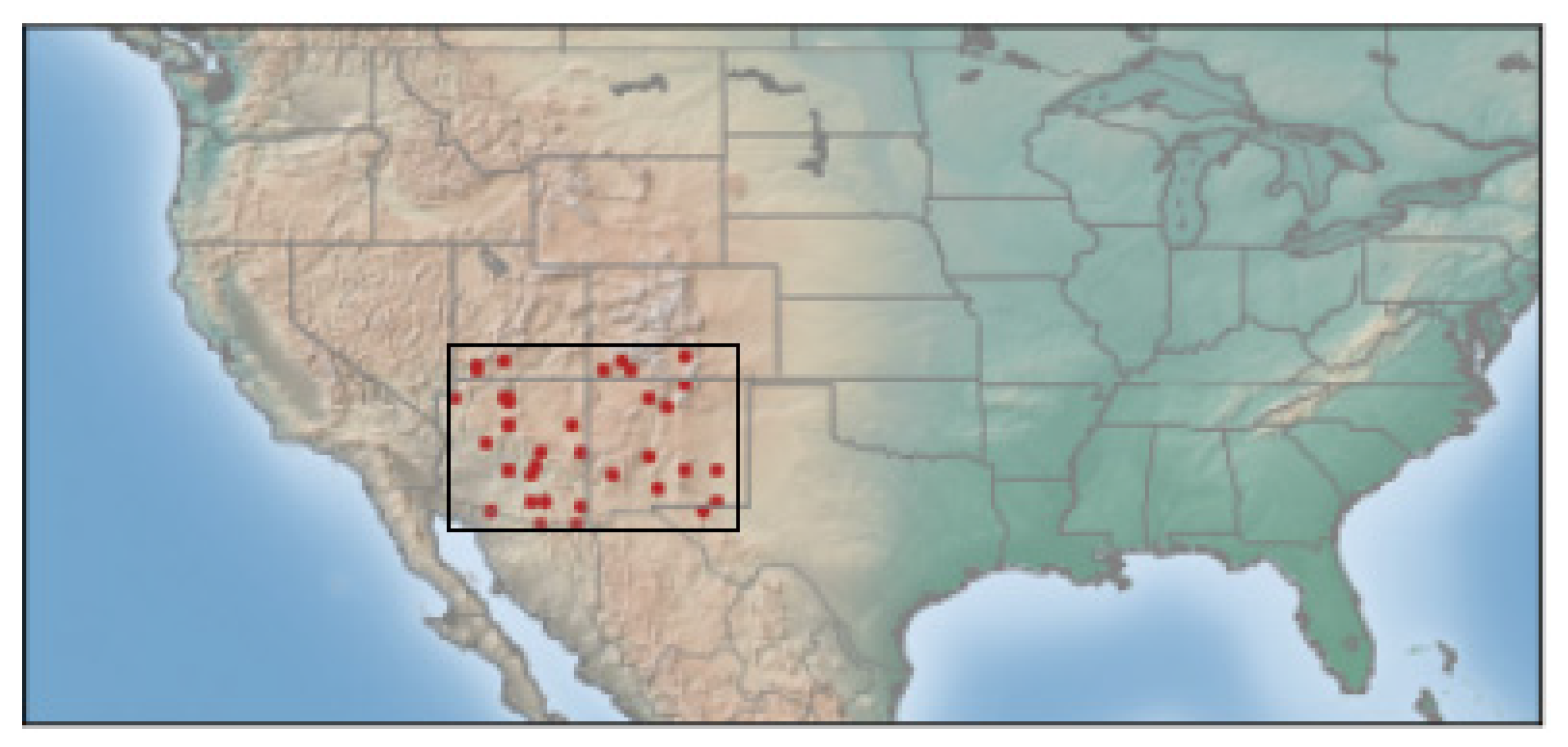
2.1. Study Area and Data

The Southwestern US is a prominent dust source [19]. Major dust sources over the region are the Chihuahuan Desert, the Colorado River, and the High Plains. Observed near-surface dust concentrations over the Southwestern USA are available from the Interagency Monitoring of Protected Visual Environments (IMPROVE) network ([20]; available online: https://views.cira.colostate.edu/fed/Express/ImproveData.aspx (accessed on 10 April 2022). The IMPROVE stations (Figure 1) have provided fine and coarse dust measurements since 1988. The sampler vacuum pump is run for 24 h and collects the dust (in µg/m³). Observations were performed every Saturday and Wednesday prior to 2001. Since then, the dust has been measured every third day, continuing to the present time.

Previous studies show that dust emissions over the Southwestern US are strongly correlated with drought [4], wind speed [13], and affected by climatic teleconnection [14]. Therefore, six meteorological and climatic factors that explain dust emissions, precipitation (pr); the 2 m air temperature; the near-surface (10 m) wind speed; the El Niño–Southern Oscillation (ENSO); the Pacific Decadal Oscillation (PDO); and the North Atlantic Oscillation (NAO), were chosen as predictors. Measurements of the monthly total precipitation, average 2 m air temperature, and 10 m wind speed were taken from the North American Regional Reanalysis (NARR) ([21]: available online: https://psl.noaa.gov/data/gridded/data.narr.monolevel.html (accessed on 10 April 2022)), available at 0.3° × 0.3° resolution. ENSO (Nino3.4), PDO, and NAO indices were taken from the National Oceanic and Atmospheric Administration (NOAA: available online: https://psl.noaa.gov/data/climateindices/list/ (accessed on 10 April 2022)). The most IMPROVE sites are located on federal lands and national parks that are often not at the center of the dust sources. Therefore, studies on the relationship between dust and meteorology are performed on a regional scale rather than on a grid/station scale (e.g., [4,18]). We performed analysis using regional dust intensity, total precipitation, average air temperature, and average wind speed averaged over the region (Figure 1). We used monthly average dust concentrations from 1988 to 2010 as training data and those from 2011 to 2020 as test data.

2.2. Machine-Learning (ML) Models

The performance of different ML algorithms was tested: (1) Multiple Linear Regression (MLR), (2) Support Vector Machine (SVM), (3) Random Forest (FR), (4) Bayesian Regularized Neural Networks (BRNN), and (5) Cubist (Cu). These models have been used previously to predict atmospheric aerosols (e.g., [22,23]). ML models were implemented in R ([24].

2.2.1. Multiple Linear Regression (MLR)

Regression analyses are widely used to describe the linear relationship between a response variable and one or more explanatory variables [25]. The MLR equation is as follows:

$$yi={\beta }_o+{\beta }_1{x}_{1i}+{\beta }_2{x}_{2i}+\dots +{\beta }_p{x}_{pi}+\epsilon$$

(1)

where i = n observations, y = dependent/response variable, x = independent/explanatory variables, ${\beta }_{\mathrm{o}}$ = y-intercept, and $\epsilon$ = the model’s residuals/errors.

2.2.2. Support Vector Machine (SVM)

SVMs are supervised learnings used for both classification and regression [26]. SVM regression is often called Support Vector Regression (SVR) in the literature. SVM has two layers, where weights are non-linear in the first layer and linear in the second layer [27,28,29,30]. The SVM decision function is represented as

$$f\left(x\right)=\omega .\mathsf{\phi }\left(x\right)+b$$

(2)

where non-linear function $\mathsf{\phi }(.)$ maps $x$ into a feature space, $\omega$ and $b$ are parameters to be determined by maximizing their objective functions, and N is the number of observations. The parameters are estimated by minimizing the sum of the empirical risk (the first term of Equation (3)) and the complexity term (the second term of Equation (3)):

$$R=C{\displaystyle \sum }_{i=1}^n{L}_{\epsilon }\left(f\left(x_i\right),y_i\right) \frac{1}{2} {\left|\left|\omega \right|\right|}^2$$

(3)

$$L_{\epsilon }\left(f\left(x_i\right),y_i\right)=\{\begin{array}{c}0 for \left|f\left(x\right)-y\right|<ϵ \\ else \left|f\left(x\right)-y\right|-ϵ \end{array}$$

(4)

where C is a positive constant that determines the trade-off between the model complexity and the extent up to which model errors larger than $ϵ$ are tolerated, ${\left|\left|\omega \right|\right|}^2$ is the regularization term denoting the Euclidian norm, and $L_{\epsilon }$ is the loss function that is insensitive to $ϵ$ and has the advantage that all data are not necessary to describe the regression vector $\omega$. The radial basis kernel functions are more suitable for handling non-linear problems and have fewer tunable parameters [31].

2.2.3. Random Forest (RF)

RF is a non-parametric algorithm within a decision tree [32]. RF consists of a combination of decision trees fitted by randomly selected subsets samples from training data. The RF algorithm builds a K number of regression trees from an (x) input vector. After K such trees ${\left\{T\left(x\right)\right\}}_1^k$ are grown, RF predictions are made as the average of all trees [33] expressed as:

$$f_{fr}^K\left(x\right)=\frac{1}{K}{\displaystyle \sum }_{k=1}^{K}T\left(x\right)$$

(5)

2.2.4. Bayesian Regularized Neural Networks (BRNN)

The BRNN comprises an artificial neural network (ANN) and the Bayesian method to estimate optimal parameters. The complex model is penalized in the Bayesian framework and reduces the overfitting problem [34,35]. BRNN imposes prior distributions on the parameters of the model. The following objective function is minimized based on gradient optimization to estimate parameters [36]:

$$F={ \mathsf{\beta }\mathrm{E}}_{\mathrm{D}}\left(\mathrm{D}|\mathrm{w}, \mathrm{M}\right)+{\mathsf{\alpha }\mathrm{E}}_{\mathrm{w}}\left(\mathrm{w}|\mathrm{M}\right)$$

(6)

where ${\mathrm{E}}_{\mathrm{D}}$ is the sum of squared errors, $\mathrm{M}$ is the ANN model, $\mathrm{Ew}\left(\mathrm{w}|\mathrm{M}\right)$ is squared ANN architecture weights, $\mathsf{\alpha } \mathrm{and} \mathsf{\beta }$ are objective function parameters, and $\mathsf{\alpha }\mathrm{Ew}$ shows weight decay ($\mathsf{\alpha }$ is a decay coefficient). $\mathrm{W}$ should be smaller to reduce the overfitting tendency.

2.2.5. Cubist (Cu)

The non-parametric Cu method is based on the rule-based model tree proposed by Quinlan [37,38,39,40]. The Cu models linearly combine two models [41]. The Cu model combines the prediction from the current model and the parent model above it in the tree [41,42].

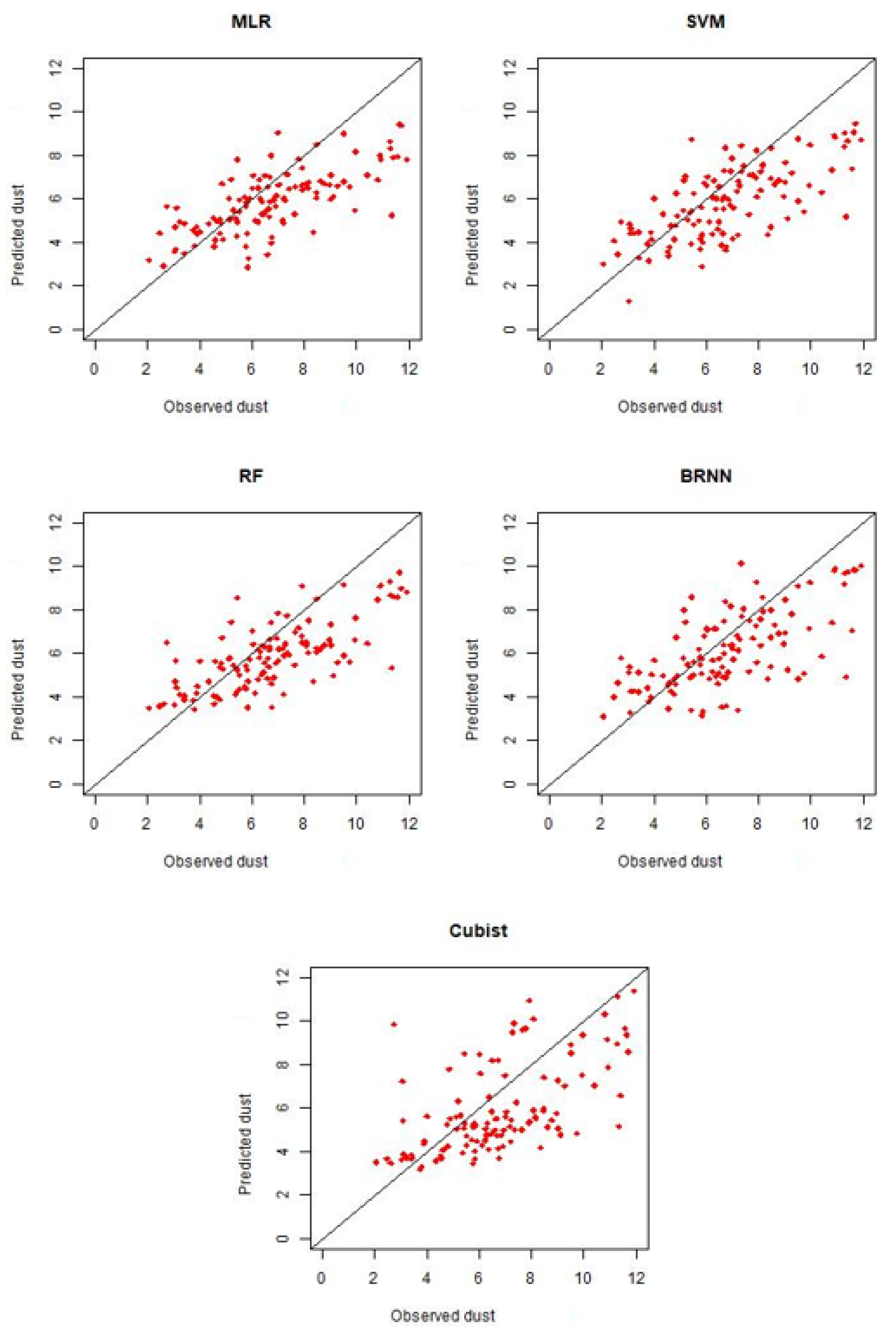
3. Results and Discussion

The ML models’ performance in predicting fine dust and coarse dust is shown in

Table 1. Performance of ML models in predicting fine dust and coarse dust (test data: 2011–2020).

ML Model	Fine Dust (PM2.5)		Coarse Dust (PM2.5–10)
	Corr (r)	RMSE (µg/m3)	Corr (r)	RMSE (µg/m3)
MLR	0.73	0.46	0.71	2.12
SVM	0.75	0.47	0.67	2.27
RF	0.81	0.40	0.71	2.08
BRNN	0.75	0.48	0.70	2.12
Cubist	0.65	0.53	0.70	2.18

. The correlation (r) of the ML-model predicted and -observed dust concentration from 2011 to 2020 ranged from 0.65 to 0.81, and the root mean square error (RMSE) ranged from 0.40 µg/m³ to 0.48 µg/m³ for fine dust. Similarly, for coarse dust, the correlation varied from 0.67 to 0.71, and the RMSE varied from 2.08 µg/m³ to 2.27 µg/m³. The correlations for fine dust were greater than the correlations for coarse dust, implying that ML models better predict fine dust than they do coarse dust.

The scatter plots of observed and predicted dust are shown in Figure 2 and Figure 3 for fine dust and coarse dust, respectively. For fine dust, all ML models underestimated high concentrations of dust. The Cubist model, compared to other models, largely underestimated both high and low dust concentrations. As with the fine dust (Figure 2), ML models underestimated high concentrations of coarse dust (Figure 3).

Machine learning algorithms show great potential (with correlations > 0.65) for predicting dustiness in the Southwestern US. ML models work better for predicting fine dust than for predicting coarse dust. Studies show that the earth system model (ESM) estimated fine dust emissions at less than 10% of the total dust emissions, and earth system models perform poorly in simulating coarse dust [2]. The poor performance of ML models in predicting coarse dust is most likely due to the short transport distance and short retention of coarse dust in the air. The IMPROVE observation stations are located on federal lands and national parks far from the dust sources [20]. The IMPROVE stations are more likely to miss the coarse dust. Therefore, regional meteorology cannot explain the variability of coarse dust. ML models also underestimate high-concentration dust events for both fine and coarse dust events. The high concentration of dust often occurs as a result of thunderstorm outflow winds/wind gusts from deep convection [43] that cannot be fully captured by the monthly average wind speed.

The relative importance of the predictor variable was calculated based on the percentage increase in RMSE without that particular variable as a predictor [23] and is shown in Figure 4. Temperature and precipitation are more important in predicting regional dustiness over the Southwestern US region for both fine dust and coarse dust. Climatic teleconnection (ENSO, PDO, and NAO) are more important predictors of coarse dust than fine dust.

Previous studies have shown that bareness is the most important factor for dust variability over the region (e.g., Figure 6 in [13] and Figure 3 in [18]). The amount of bareness or vegetation of a region depends on both precipitation and temperature. In this study, we saw the relative importance of temperature and precipitation in dust emissions. Reduced precipitation promoted lower soil moisture, leading to more intense dust emissions. The opposite was true for temperature. On a monthly timescale, as in this study, dust emissions strongly respond to temperature due to soil moisture depletion in topsoil. The impacts of precipitation on dust emissions are stronger on a longer timescale (i.e., annual) due to changes in vegetation cover [44].

4. Conclusions

This study investigated several machine-learning (ML) models’ abilities to predict aeolian dust over the Southwestern US. The observed dust was taken from the Interagency Monitoring of Protected Visual Environments (IMPROVE) network while the regional meteorology data (precipitation, temperature, wind speed) were retrieved from North American Regional Reanalysis (NARR). The models’ performances for fine dust and coarse dust were compared. Then, the relative importance of the predictors was assessed. The main conclusions from this study can be summarized as follows:

• The non-linear models performed better than linear regression to predict both fine and coarse dust. All ML models underestimated high concentrations of dust.
• ML models better predicted fine dust than coarse dust over the study region.
• The air temperature was the most important meteorological variable, followed by precipitation, for predicting monthly dust over the region.

The Southwestern US region is likely to see severe drought due to both reduced precipitation and increased temperatures [45] reducing surface moisture and vegetation, which enhance erodibility and dust emissions. Temperature and precipitation, being the most important predictors, imply the presence of future, warming-enhanced drought [46,47] over the region, associated with increased dust emissions and the related severe health and environmental concerns. ML models show the potential for predicting dustiness over the region, helping effective mitigation efforts.

References

1. Prospero, J.M.; Collard, F.X.; Molinié, J.; Jeannot, A. Characterizing the annual cycle of African dust transport to the Caribbean Basin and South America and its impact on the environment and air quality. Glob. Biogeochem. Cycles 2014, 28, 757–773. [Google Scholar] [CrossRef]
2. Kok, J.F.; Ward, D.S.; Mahowald, N.M.; Evan, A.T. Global and regional importance of the direct dust-climate feedback. Nat. Commun. 2018, 9, 241. [Google Scholar] [CrossRef] [PubMed]
3. Evans, S.; Malyshev, S.; Ginoux, P.; Shevliakova, E. The impacts of the dust radiative effect on vegetation growth in the Sahel. Glob. Biogeochem. Cycles 2019, 33, 1582–1593. [Google Scholar] [CrossRef]
4. Achakulwisut, P.; Mickley, L.J.; Anenberg, S.C. Drought-sensitivity of fine dust in the US Southwest: Implications for air quality and public health under future climate change. Environ. Res. Lett. 2018, 13, 054025. [Google Scholar] [CrossRef]
5. Bhattachan, A.; Okin, G.S.; Zhang, J.; Vimal, S.; Lettenmaier, D.P. Characterizing the role of wind and dust in traffic accidents in California. Geo. Health 2019, 3, 328–336. [Google Scholar] [CrossRef] [PubMed] [Green Version]
6. Al-Hemoud, A.; Al-Dousari, A.; Misak, R.; Al-Sudairawi, M.; Naseeb, A.; Al-Dashti, H.; Al-Dousari, N. Economic impact and risk assessment of sand and dust storms (SDS) on the oil and gas industry in Kuwait. Sustainability 2019, 11, 200. [Google Scholar] [CrossRef] [Green Version]
7. Javadian, M.; Behrangi, A.; Sorooshian, A. Impact of drought on dust storms: Case study over Southwest Iran. Environ. Res. Lett. 2019, 14, 124029. [Google Scholar] [CrossRef]
8. Arcusa, S.H.; McKay, N.P.; Carrillo, C.M.; Ault, T.R. Dust—Drought Nexus in the Southwestern United States: A Proxy—Model Comparison Approach. Paleoceanogr. Paleoclimatol. 2020, 35, e2020PA004046. [Google Scholar] [CrossRef]
9. Munson, S.M.; Belnap, J.; Okin, G.S. Responses of wind erosion to climate-induced vegetation changes on the Colorado Plateau. Proc. Natl. Acad. Sci. USA 2011, 108, 3854–3859. [Google Scholar] [CrossRef] [Green Version]
10. Bestelmeyer, B.T.; Peters, D.P.; Archer, S.R.; Browning, D.M.; Okin, G.S.; Schooley, R.L.; Webb, N.P. The grassland–shrubland regime shift in the southwestern United States: Misconceptions and their implications for management. BioScience 2018, 68, 678–690. [Google Scholar] [CrossRef] [Green Version]
11. Hand, J.L.; Gill, T.E.; Schichtel, B.A. Spatial and seasonal variability in fine mineral dust and coarse aerosol mass at remote sites across the United States. J. Geophys. Res. Atmos. 2017, 122, 3080–3097. [Google Scholar] [CrossRef]
12. Achakulwisut, P.; Shen, L.; Mickley, L.J. What controls springtime fine dust variability in the western United States? Investigating the 2002–2015 increase in fine dust in the US Southwest. J. Geophys. Res. Atmos. 2017, 122, 12–449. [Google Scholar] [CrossRef]
13. Pu, B.; Ginoux, P. How reliable are CMIP5 models in simulating dust optical depth? Atmos. Chem. Phys. 2018, 18, 12491–12510. [Google Scholar] [CrossRef] [Green Version]
14. Okin, G.S.; Reheis, M.C. An ENSO predictor of dust emission in the southwestern United States. Geophys. Res. Lett. 2002, 29, 46-1–46-3. [Google Scholar] [CrossRef]
15. Witten, I.H.; Frank, E. Data mining: Practical machine learning tools and techniques with Java implementations. Acm Sigmod Rec. 2002, 31, 76–77. [Google Scholar] [CrossRef]
16. Lee, J.; Shi, Y.R.; Cai, C.; Ciren, P.; Wang, J.; Gangopadhyay, A.; Zhang, Z. Machine learning-based algorithms for global dust aerosol detection from satellite images: Inter-comparisons and evaluation. Remote Sens. 2021, 13, 456. [Google Scholar] [CrossRef]
17. Ebrahimi-Khusfi, Z.; Nafarzadegan, A.R.; Dargahian, F. Predicting the number of dusty days around the desert wetlands in southeastern Iran using feature selection and machine learning techniques. Ecol. Indic. 2021, 125, 107499. [Google Scholar] [CrossRef]
18. Pu, B.; Ginoux, P. Projection of American dustiness in the late 21st century due to climate change. Sci. Rep. 2017, 7, 1–10. [Google Scholar] [CrossRef] [Green Version]
19. Ginoux, P.; Prospero, J.M.; Gill, T.E.; Hsu, N.C.; Zhao, M. Global—scale attribution of anthropogenic and natural dust sources and their emission rates based on MODIS Deep Blue aerosol products. Rev. Geophys. 2012, 50, 1–36. [Google Scholar] [CrossRef]
20. DeBell, L.J.; Gebhart, K.A.; Hand, J.L.; Malm, W.C.; Pitchford, M.L.; Schichtel, B.A.; White, W.H. Spatial and Seasonal Patterns and Temporal Variability of Haze and Its Constituents in the United States: Report IV. CIRA, Cooperative Institute for Research in the Atmosphere, Colorado State University. 2006. Available online: https://hero.epa.gov/hero/index.cfm/reference/details/reference_id/3121718 (accessed on 10 April 2022).
21. Mesinger, F.; DiMego, G.; Kalnay, E.; Mitchell, K.; Shafran, P.C.; Ebisuzaki, W.; Jović, D.; Woollen, J.; Rogers, E.; Berbery, E.H.; et al. North American regional reanalysis [Dataset]. Bull. Am. Meteorol. Soc. 2006, 87, 343–360. [Google Scholar] [CrossRef] [Green Version]
22. Xu, Y.; Ho, H.C.; Wong, M.S.; Deng, C.; Shi, Y.; Chan, T.C.; Knudby, A. Evaluation of machine learning techniques with multiple remote sensing datasets in estimating monthly concentrations of ground-level PM2. 5. Environ. Pollut. 2018, 242, 1417–1426. [Google Scholar] [CrossRef] [PubMed]
23. Gholami, H.; Mohamadifar, A.; Sorooshian, A.; Jansen, J.D. Machine-learning algorithms for predicting land susceptibility to dust emissions: The case of the Jazmurian Basin, Iran. Atmos. Pollut. Res. 2020, 11, 1303–1315. [Google Scholar] [CrossRef]
24. R Core Team. R: A Language and Environment for Statistical Computing; R Foundation for Statistical Computing: Vienna, Austria, 2013. Available online: http://www.R-project.org/ (accessed on 19 April 2022).
25. Helsel, D.R.; Hirsch, R.M. Statistical Methods in Water Resources; Elsevier: Amsterdam, The Netherlands, 1992; Volume 49. [Google Scholar]
26. Vapnik, V. The Nature of Statistical Learning Theory; Springer: Berlin/Heidelberg, Germany, 1999. [Google Scholar]
27. Bray, M.; Han, D. Identification of support vector machines for runoff modelling. J. Hydroinform. 2004, 6, 265–280. [Google Scholar] [CrossRef] [Green Version]
28. Noble, W.S. What is a support vector machine? Nat. Biotechnol. 2006, 24, 1565–1567. [Google Scholar] [CrossRef]
29. Tabari, H.; Kisi, O.; Ezani, A.; Talaee, P.H. SVM, ANFIS, regression and climate based models for reference evapotranspiration modeling using limited climatic data in a semi-arid highland environment. J. Hydrol. 2012, 444, 78–89. [Google Scholar] [CrossRef]
30. Karandish, F.; Šimůnek, J. A comparison of numerical and machine-learning modeling of soil water content with limited input data. J. Hydrol. 2016, 543, 892–909. [Google Scholar] [CrossRef] [Green Version]
31. Hsu, C.W.; Chang, C.C.; Lin, C.J. A Practical Guide to Support Vector Classification; Department of Computer Science National Taiwan University: Taiwan, China, 2003. [Google Scholar]
32. Breiman, L. Random forests. Mach. Learn. 2001, 45, 5–32. [Google Scholar] [CrossRef] [Green Version]
33. Rodriguez-Galiano, V.; Sanchez-Castillo, M.; Chica-Olmo, M.; Chica-Rivas, M.J.O.G.R. Machine learning predictive models for mineral prospectivity: An evaluation of neural networks, random forest, regression trees and support vector machines. Ore Geol. Rev. 2015, 71, 804–818. [Google Scholar] [CrossRef]
34. Garg, D.; Mishra, A. Bayesian regularized neural network decision tree ensemble model for genomic data classification. Appl. Artif. Intell. 2018, 32, 463–476. [Google Scholar] [CrossRef]
35. Kayri, M. Predictive abilities of bayesian regularization and Levenberg–Marquardt algorithms in artificial neural networks: A comparative empirical study on social data. Math. Comput. Appl. 2016, 21, 20. [Google Scholar] [CrossRef]
36. Okut, H. Bayesian regularized neural networks for small n big p data. Artif. Neural Netw.-Models Appl. 2016, 16, 21–23. [Google Scholar]
37. Quinlan, J.R. Learning with Continuous Classes. In Proceedings of the Australian Joint Conference on Artificial Intelligence, Hobart, Australia, 16–18 November 1992; Volume 6, pp. 343–348. [Google Scholar]
38. Quinlan, J.R. Combining instance-based and model-based learning. In Proceedings of the Tenth International Conference on International Conference on Machine Learning, Amherst, MA, USA, 27–29 July 1993; Morgan Kaufmann Publishers Inc.: San Francisco, CA, USA, 1993; pp. 236–243. [Google Scholar]
39. Quinlan, J.R. Improved use of continuous attributes in C4. 5. J. Artif. Intell. Res. 1996, 4, 77–90. [Google Scholar] [CrossRef] [Green Version]
40. Houborg, R.; McCabe, M.F. A hybrid training approach for leaf area index estimation via Cubist and random forests machine-learning. ISPRS J. Photogramm. Remote Sens. 2018, 135, 173–188. [Google Scholar] [CrossRef]
41. Zhou, J.; Li, E.; Wei, H.; Li, C.; Qiao, Q.; Armaghani, D.J. Random forests and cubist algorithms for predicting shear strengths of rockfill materials. Appl. Sci. 2019, 9, 1621. [Google Scholar] [CrossRef] [Green Version]
42. John, K.; Kebonye, N.M.; Agyeman, P.C.; Ahado, S.K. Comparison of Cubist models for soil organic carbon prediction via portable XRF measured data. Environ. Monit. Assess. 2021, 193, 197. [Google Scholar] [CrossRef]
43. Brazel, A.J.; Nickling, W.G. The relationship of weather types to dust storm generation in Arizona (1965–1980). J. Climatol. 1986, 6, 255–275. [Google Scholar] [CrossRef]
44. Namdari, S.; Karimi, N.; Sorooshian, A.; Mohammadi, G.; Sehatkashani, S. Impacts of climate and synoptic fluctuations on dust storm activity over the Middle East. Atmos. Environ. 2018, 173, 265–276. [Google Scholar] [CrossRef]
45. Jeong, D.I.; Sushama, L.; Naveed Khaliq, M. The role of temperature in drought projections over North America. Clim. Chang. 2014, 127, 289–303. [Google Scholar] [CrossRef]
46. Cook, B.I.; Mankin, J.S.; Marvel, K.; Williams, A.P.; Smerdon, J.E.; Anchukaitis, K.J. Twenty-First Century Drought Projections in the CMIP6 Forcing Scenarios. Earth’s Future 2020, 8, e2019EF001461. [Google Scholar] [CrossRef] [Green Version]
47. Spinoni, J.; Barbosa, P.; Bucchignani, E.; Cassano, J.; Cavazos, T.; Christensen, J.H.; Christensen, O.B.; Coppola, E.; Evans, J.; Geyer, B.; et al. Future global meteorological drought hot spots: A study based on CORDEX data. J. Clim. 2020, 33, 3635–3661. [Google Scholar] [CrossRef]
Figure 1. Study region. The red dots indicate the IMPROVE stations.
Climate 10 00078 g001
Figure 2. Observed and predicted monthly fine dust (PM2.5 in µg/m3) from five ML models; Multiple Linear Regression (MLR), Support Vector Machines (SVM), Random Forests (RF), Bayesian Regularized Neural Networks (BRNN), and Cubist (Cu) during 2011 to 2020.
Climate 10 00078 g002
Figure 3. Observed and predicted monthly coarse dust (PM10 in µg/m3) from five ML models; Multiple Linear Regression (MLR), Support Vector Machines (SVM), Random Forests (RF), Bayesian Regularized Neural Networks (BRNN), and Cubist (Cu) during 2011 to 2020.
Climate 10 00078 g003
Figure 4. (a,b) The relative importance of predictor variables (RF model). Y-axis shows the percentage change in RMSE for predicting dust without using the corresponding variable as a predictor; (c) Variable inflation factor to check the multicollinearity in the prediction models. Precipitation (P), air temperature (T), wind speed (W).
Climate 10 00078 g004