Semiparametric Estimation of a Corporate Bond Rating Model

Abstract

This paper investigates the incentive of credit rating agencies (CRAs) to bias ratings using a semiparametric, ordered-response model. The proposed model explicitly takes conflicts of interest into account and allows the ratings to depend flexibly on risk attributes through a semiparametric index structure. Asymptotic normality for the estimator is derived after using several bias correction techniques. Using Moody’s rating data from 2001 to 2016, I found that firms related to Moody’s shareholders were more likely to receive better ratings. Such favorable treatments were more pronounced in investment grade bonds compared with high yield bonds, with the 2007–2009 financial crisis being an exception. Parametric models, such as the ordered-probit, failed to identify this heterogeneity of the rating bias across different bond categories.

1. Introduction

While the Credit Rating Agencies’ (CRA) profits exploded with the growth of structured finance, the collapse of highly rated securities in the 2007–2009 financial crisis led to suspicions that the ratings were perhaps “too optimistic” during the boom years. One prevailing explanation for rating inflation is the perceived conflicts of interest. A long-standing conflict stems from the “issuer-paid” model, whereby CRAs are paid by the issuers seeking ratings and, hence, are incentivized to issue inflated ratings.1

In the past two decades, rating agencies have been increasingly owned by large financial institutions, which induces a conflict of interest that is less obvious: CRAs may inflate ratings to benefit issuers that are related to their shareholders. While much of the extant literature has focused on issuer-paid models, this paper examines the empirical relationship between rating inflation and this often-neglected source of conflicts of interest—what I call shared-ownership—within a novel econometric framework.

Credit ratings are determined by a plethora of issuer- and issue-level characteristics. The proposed model has a multiple-index structure, which allows ratings to depend on different classes of characteristics in a non-separable fashion. Three indices are employed to represent firm characteristics, bond characteristics, and the Moody-firm-ownership-index (MFOI), which is a shared-ownership index that I introduce later in this paper. As the model is estimated semiparametrically, it is not necessary to know how CRAs utilize these characteristics to assign ratings a priori to ensure consistent estimation.

While there are numerous studies on single-index models in the econometric literature,2 only a handful of studies are available on the estimation of multiple-index regression models. Identification results of multiple-index models were first established by Ichimura and Lee (1991) and Horowitz (1998), where the authors used semiparametric least squares (SLS) to estimate the index parameters. Donkers and Schafgans (2008) proposed a derivate-based estimation method to avoid the need to pre-specify the number of indices. A recent study, Ahn et al. (2017), proposed to estimate the index coefficients (up to scale) based on an eigenvalue approach.

Studies in the statistical literature, such as Xia et al. (2002) and Xia (2008), also employ different variants of multiple-index models to flexibly reduce the data dimension. All the aforementioned studies, with the exception of Ichimura and Lee (1991), required estimating nonparametric conditional mean functions and/or derivatives in the original space of regressors. Consequently, such methods may not behave well when the sample size is small relative to the number of regressors. This paper, in contrast, extends the maximum likelihood approach of Klein and Sherman (2002) to estimate the index parameters directly in a low dimension space spanned by the three indices. To the best of my knowledge, this is also the first study in estimating a multipe-index model where the dependent variable is ordinal.

Ordered response models are more complicated than ordinary regression setting in that there is no conditional mean function to analyze: the outcome variable, y, is merely a “label” for the ordered, nonquantitaive outcomes. In order to interpret the model, one typically refers to the probabilities themselves. This paper employs a multivariate kernel density estimator for the semiparametric rating probability function. Bias-reducing kernels are often used in the literature to ensure the estimators have an appropriately low order of bias, which is required to establish their asymptotic results conveniently. However, when the object of interest is a probability, these bias reducing kernels can deliver an estimated probability outside of [0, 1] and render the estimation results difficult to interpret. To circumvent this challenge, I obtain alternative bias reduction via a “recursive differencing” strategy proposed by Shen and Klein (2019) and then establish $\sqrt{N}$ normality for the proposed estimator. 3

Using the Mergent’s Fixed Income Securities Database (FISD) for the years 2001 to 2016, I estimate Moody’s rating model year-by-year and characterize the average partial effects (APE) of MFOI, the aforementioned shared-ownership index. In a seminal paper, Kedia et al. (2017) found that the average rating for a Moody-related firm was 0.213 notch better than a comparable non-Moody-related firm for the period of 2001–2010.

As the employed model permits the partial effect of MFOI to flexibly depend on other characteristics in an interactive fashion, the contribution of this application to the pertaining empirical literature is to explore the heterogeneity of rating bias. The APE of MFOI is more pronounced in investment grade bonds than in high yield bonds; however, this pattern reversed during the 2007–2009 financial crisis, implying that high yield bonds were more likely to receive favorable ratings due to a closer liaison with Moody’s. A placebo test based on “false owners” revealed that the salient partial effects of MFOI were indicative of Moody’s bias toward firms related to its own shareholders.

The rest of this paper is organized as follows: In Section 2, I introduce the proposed measure of shared-ownership and the firm/bond characteristics that are employed in the model. Section 3 describes the model and the estimation strategy. Section 4 reports the results from simulation designs and the empirical data. Section 5 concludes this study. In Appendix A, I state the asymptotic properties for the proposed estimator and the assumptions required to establish them. The formal proofs and intermediate lemmas are contained in the Online Supplemental Material.

2. Data and Variable Construction

I formulate a model to investigate Moody’s ratings on corporate bonds at issuance (e.g., initial ratings) from 2001, when Moody’s went public, to 2016. From Mergent’s Fixed Income Securities Database (FISD), I obtain initial ratings on corporate bonds issued by public firms covered by either the Center for Research in Security Prices (CRSP) or Compustat. There is a distinction between the issuer rating and issue rating for corporate bonds. The former addresses the issuer’s overall credit creditworthiness and usually applies to senior unsecured debt, whereas the latter refers to specific debt obligations and considers the ranking in the capital structure such as secured or subordinated.

This paper builds a model for issue ratings; therefore, both firm and bond characteristics are considered as explanatory variables.4 Descriptions and summary statistics of these characteristics are provided in

Table 1. Summary Statistics: A number of firm and bond characteristics were selected to predict credit ratings based on Baghai et al. (2014) and Kedia et al. (2017): (1) the value of the firm’s total assets (log(asset)), (2) long- and short-term debt divided by total assets (Book_lev). (3) Convertible debt divided by total assets (ConvDe_assets), (4) rental paymetns divided by total assets (Rent_Assets), (5) cash and marketable securities divided by total assets (Cash_assets), (6) long- and short-term debt divided by EBITDA (Debt_EBITDA), (7) EBITDA to interest payments (EBITA_int), (8) profitability, measured as EBITDA divided by sales (Profit), (9) tangibility, measured as net property, plant, and equipment divided by total assets (PPE_assets), (10) capital expenditures divided by total assets (CAPX_assets), (11) the volatility of profitability (Vol_profit), (12) the log of the issuing amount (log(issuing amount)), (13) a dummy variable indicating whether the bond is senior (seniority), and (14) a dummy variable indicating whether the bond is secured (security).

	Investment Grade		High-Yield
	Mean	Std.Dev.	Mean	Std.Dev.
Firm Characteristics
log(asset)	10.88	1.92	8.26	1.45
book_lev	0.33	0.18	0.44	0.20
convDe_asset	0.01	0.03	0.03	0.07
rent_asset	0.01	0.01	0.02	0.03
cash_asset	0.11	0.12	0.08	0.09
debt_ebitda	4.95	11.16	4.45	20.76
ebitda_int	14.45	31.30	4.82	5.91
profit	0.31	0.28	0.03	8.38
PPE_asset	0.23	0.26	0.37	0.28
CAPEX_asset	0.03	0.04	0.07	0.10
profit_vol	0.06	1.84	−0.92	41.74
Bond Characteristics
log(issuing amount)	12.69	1.69	12.66	0.73
seniority	0.93	0.26	0.69	0.46
security	0.01	0.06	0.09	0.00

. Other than the standard firm-level characteristics, three bond characteristics are included: whether the bond is a senior security, the security level (collateralized by an asset or not), and the issue amount. All three characteristics are relevant to the loss on bond holders should a default event occur. After combining data from multiple sources, the final sample was composed of 10,557 bonds issued by 1370 firms.

Measuring Conflicts of Interest

One lesson that investors and policy makers learned in the 2007–2009 financial crisis is that credit ratings are contaminated with conflicts of interest. CRAs with large market shares, such as Moody’s and Standard & Poor’s, are increasingly owned by large institutional investors, making their role as an unbiased financial market “gatekeeper” ever more suspicious.5 As noted by Kedia et al. (2017), large shareholders of credit rating agencies have economic incentives to influence the rating process. Specifically, they find Moody’s ratings on bonds issued by important investee firms of its two stable large shareholders6 are more favorable relative to ratings from S&P and Fitch.

To construct a measure for the “connectedness” between a bond issuer and Moody’s through common shareholders, I first obtained the list of Moody’s shareholders from Thomson Reuters (13F) in each quarter from 2001Q1–2016Q4. From Moody’s perspective, the economic interest of some shareholders were clearly more important than others. I approximate each shareholder j’s “influence” on Moody’s by the percentage of Moody’s stock that it holds, ${\lambda }_j$. Next, I obtained the portfolio weight of bond issuer i in shareholder j’s investment portfolio, termed $p_{ij}$. The shareholder’s manager type code (MGRNO) and the firm’s Committee on Uniform Securities Identification Procedures (CUSIP) number were used to match the shareholding data with the 1370 bond issuers.

Based on the information collected above, I construct the following variable, termed the Moody-Firm-Ownership-Index (MFOI), to summarily characterize a bond issuer i’s liaison with Moody’s shareholders,

$$\begin{array}{c}\hfill MFO{I}_i=\sum _{j=1}^M{p}_{ij}{\lambda }_j,{\mathrm{Moody}}^{\prime }\mathrm{s}\mathrm{has}j=1,2,\cdots ,M\mathrm{shareholders}\end{array}$$

(1)

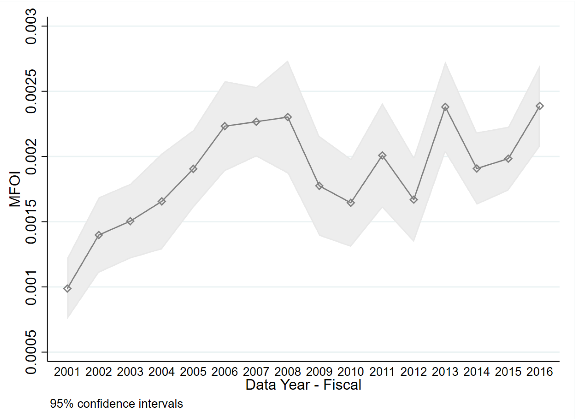
Figure 1 provides an illustration on how this formula works. Assume that Moody’s has only two shareholders: Berkshire Hathaway, which owns 15% of Moody’s stocks, and Goldman Sachs, which owns 3% of Moody’s stocks. There are three bond issuers indexed by $i,j,k$, and two of which are invested by the two aforementioned shareholders of Moody’s. Specifically, the value of issuer i’s equity accounts for 20% of Berkshire Hathaway’s portfolio and each of issuer i’s and j’s accounts for 10% of Goldman Sach’s portfolio. For these three issuers, $MFO{I}_i=15\%\times 20\%+3\%\times 10\%=0.033,MFO{I}_j=3\%\times 10\%=0.003,$ and $MFO{I}_k=0$. As can be seen from Figure 2, bond issuers had increasingly strong connections with Moody’s prior to the financial crisis, as measured by the average of MFOI.

Then what empirical relation is expected between the MFOI and credit ratings? By construction, a bond issuer i has a larger MFOI in two instances. First, when some of Moody’s shareholders increases their stakes in firm i due to favorable private information, $p_{ij}$ increases for those shareholders and leads to a larger MFOI. One would anticipate the ratings to go up to reflect such favorable information. Secondly, the MFOI also tends to be large when the common shareholder has a strong influence over Moody’s (e.g., ${\lambda }_j$ is large). Moody’s might have a greater incentive to assign favorable ratings. In both cases, a larger MFOI intuitively leads to a higher credit ratings. Below I present an econometric model to quantify the impact of MFOI on ratings.

3. Empirical Model

3.1. Model and Motivation for the Estimator

Credit ratings are discrete, ordered indicators of the credit worthiness of corporate bonds. Under Moody’s rating scale, the observed bond rating $Y_i$ takes a value from 1 to 7,7 and is related to a bond’s latent default risk $y_i^{*}$ as follows

$$\begin{array}{ccc}\hfill Y_i& =& \left\{\begin{array}{cc}1\hfill & \mathrm{if}{T}_0<y_i^{*}<T_1\hfill \\ 2\hfill & \mathrm{if}{T}_1\le y_i^{*}<T_2\hfill \\ ⋮\hfill \\ 7\hfill & \mathrm{if}{T}_6\le y_i^{*}<T_7\hfill \end{array}\right.\hfill \end{array}$$

(2)

with the $T_j$ being parameters such that $-\infty =T_0<T_1<T_2<\cdots <T_6<T_7=\infty$. Thus, the range of default risk $y_i^{*}$ is partitioned into seven mutually exclusive and exhaustive intervals, and the numerical rating $Y_i$ indicates the interval into which a particular bond’s credit quality falls. The higher the default risk is, the lower the credit rating is. Consider the following model for $y_i^{*}$,

$$\begin{array}{c}\hfill y_i^{*}=g({\mathbf{X}}_i,S_i)\end{array}$$

(3)

where ${\mathbf{X}}_i=[{\mathbf{F}}_i,{\mathbf{B}}_i,MFO{I}_i]$.8 For each bond i, assume ${\mathbf{F}}_i=(F_{1i},F_{2i},\cdots )\in {\mathcal{R}}^{\mathcal{F}}$ is a vector of firm characteristics, ${\mathbf{B}}_i=(B_{1i},B_{2i},\cdots )\in {\mathcal{R}}^{\mathcal{B}}$ is a vector of the bond characteristics, and $MFO{I}_i$ is the aforementioned measure of conflicts of interest. The model allows for both continuous as well as discrete characteristics. $S_i$ is a scalar error term summarizing private information, which the rating agency takes into account but is not observed to the econometrician. Instead of making distributional assumption about S, as with an ordered-probit model (OPM), I make an index assumption that will be provided below.

With $Y_{ik}=\mathbf{1}\{Y_i=k\}$, a key object of estimation interest is $P_{ik}\equiv Pr(Y_{ik}=1|{\mathbf{X}}_{\mathbf{i}})$, which is the probability that a bond will be rated in category k conditional on the vector of explanatory variables. In order to estimate the above probability with a moderately sized sample, I define two indices,

$$\begin{array}{ccc}\hfill \mathit{Firm}\mathit{Index}:W_{Fi}& \equiv & F_{1i}{\beta }_{10}^F+F_{2i}{\beta }_{20}^F+\cdots \hfill \end{array}$$

(4)

$$\begin{array}{ccc}\hfill \mathit{Bond}\mathit{Index}:W_{Bi}& \equiv & B_{1i}{\beta }_{10}^B+B_{2i}{\beta }_{20}^B+\cdots \hfill \end{array}$$

(5)

and make the following assumption,

$$\begin{array}{ccc}\hfill Pr(Y_{ik}=1|{\mathbf{X}}_i)& =& Pr(Y_{ik}=1|W_{Fi},W_{Bi},MFO{I}_i),\mathrm{for}k=1,2,\cdots ,7\hfill \\ \hfill & \equiv & P_k(W_{Fi},W_{Bi},MFO{I}_i)\hfill \end{array}$$

(6)

The employed approach is semiparametric because firm and bond characteristics enter the rating function as two parametric indices ($W_{Fi}$ and $W_{Bi}$, respectively) whereas the main variable of interest, $MFO{I}_i$, enters the rating function nonparametrically by itself.

In the empirical literature of bond rating, another prevailing approach to estimate the rating probability is the ordered-probit model (OPM), which assumes

$$\begin{array}{c}\hfill y_i^{*}=X_i{\beta }_0+S_i,S_i\sim \mathcal{N}(0,1)\end{array}$$

(7)

Given the normality of S, the parametric counterpart of (6) is a known function of $X_i{\beta }_0$ that does not vary across categories.9 Compared to OPM, the link function $P_k(·,·,·)$ in the proposed semiparametric model (SIM) is left unknown and estimated nonparametrically. Therefore, researchers do not need to take a stand on the fashion that ratings depend on firm characteristics, bond characteristics, and conflicts of interest. Moreover, $P_k(·,·,·)$ is category-specific and permits the rating agency to employ different rating criteria for each rating category.

3.2. Estimation Strategy

In the SIM described by Equations (4)–(6), the slope coefficients in the firm and bond indices, ${\beta }^F$ and ${\beta }^B$, can only be identified up to location and scale.10 Consequently, I normalize the coefficient of a firm characteristics $F_1$ and a bond characteristics $B_1$ to one and define the normalized indices as:

$$\begin{array}{ccc}\hfill \mathit{Normalized}\mathit{Firm}\mathit{Index}:V_{Fi}& \equiv & W_{Fi}/{\beta }_{10}^F=F_{1i}+F_i^{\prime }{\theta }_0^F\hfill \\ \hfill \mathit{Normalized}\mathit{Bond}\mathit{Index}:V_{Bi}& \equiv & W_{Bi}/{\beta }_{10}^B=B_{1i}+B_i^{\prime }{\theta }_0^B\hfill \end{array}$$

(8)

where ${\theta }_0^F=({\beta }_{20}^F/{\beta }_{10}^F,{\beta }_{30}^F/{\beta }_{10}^F,\cdots )$ and ${\theta }_0^B=({\beta }_{20}^B/{\beta }_{10}^B,{\beta }_{30}^B/{\beta }_{10}^B,\cdots )$. Note that the identifiable parameter ${\theta }_0={({\theta }_0^F,{\theta }_0^B)}^{\prime }$ captures the relative impact of other firm and bond characteristics to $F_1$ and $B_1$, respectively. Below I develop an $\sqrt{N}-$normal estimator for ${\theta }_0$.

Specifically, I employ an estimator based on an extension of the approach in Klein and Sherman (2002) that maximizes the following estimated log-likelihood function:

$$\begin{array}{ccc}\hfill \widehat{Q}\left(\theta \right)& =& \frac{1}{N}\sum _{i=1}^N{\tau }_i\left\{\sum _{k=1}^7{Y}_{ik}Ln\left(\widehat{P_k}(V_{Fi},V_{Bi},MFO{I}_i)\right)\right\}\hfill \end{array}$$

(9)

where $Y_{ik}=\mathbf{1}\{Y_i=k\}$, $\widehat{P_k}(V_{Fi},V_{Bi},MFO{I}_i)$ is a semiparametric estimator of the rating probability defined in (6), and ${\tau }_i$ is a trimming function, which is introduced to stabilize the probabilistic estimator. Based on simulation evidence, we select the trimming threshold to be the 99th percentile.

The rating probability $P_k(V_{Fi},V_{Bi},MFO{I}_i)$ describes the probability that bond i is rated as category k conditional on the three indices. Intuitively, this probability can be estimated by a weighted average of $Y_{jk}$ across a group of bonds j that have similar characteristics to bond i. That is, if most similar bonds are rated as category k, the probability of bond i receiving a rating of k should be high. In practice, econometricians use kernels, which is a function ${\mathbf{K}}_h(·)$ that is symmetric and integrated to one, to take the average around a small neighborhood around bond i. Formally, this probability is estimated as

$$\begin{array}{c}\hfill \widehat{P_k}(V_{Fi},V_{Bi},MFO{I}_i)=\frac{1}{N-1}\sum _{j\ne i}^{}{Y}_{jk}{W}_{ji},W_{ji}\equiv \frac{{\mathbf{K}}_h(V_i-V_j)}{\frac{1}{N-1}{\sum }_{j\ne i}^{}{\mathbf{K}}_h(V_i-V_j)}\end{array}$$

(10)

where $Y_{jk}$ is a binary variable indicating whether the similar bond j is rated as category k or not. The kernel function is

$$\begin{array}{c}\hfill {\mathbf{K}}_h(V_i-V_j)=\frac{1}{h_1{h}_2{h}_3}K\left(\frac{V_{Fj}-V_{Fi}}{h_1}\right)K\left(\frac{V_{Bj}-V_{Bi}}{h_2}\right)K\left(\frac{MFO{I}_j-MFO{I}_i}{h_3}\right)\end{array}$$

(11)

In this paper I use a second-order Gaussian kernel: $K\left(u\right)=\frac{1}{\sqrt{2\pi }}exp(-u^2/2)$. $\mathbf{h}\equiv {(h_1,h_2,h_3)}^{\prime }$ is a bandwidth parameter that goes to zero as sample size approaches infinity. Intuitively $\mathbf{h}$ controls the number of similar bonds that are included in the kernel-weighted average in (10). A smaller bandwidth $\mathbf{h}$ will lead to a smaller bias (only the j’s that are very similar to i are included) but a larger variance (fewer observations are included).

An important problem in practice is to select the bandwidth parameter h. I follow Silverman (1982) and set the bandwidth $h_j=0.97{\sigma }_j{N}^{-r}$, where ${\sigma }_j$ is the standard deviation of the j’th index. To ensure asymptotic normality of the proposed estimator, r must be selected in a manner such that (i) the estimated Hessian of the log-likehihood function defined in (9) converges uniformly to the expected Hessian at the true parameter values and (ii) the gradient is centered at zero (e.g., no asymptotic bias) and also converges to the true gradient.

As shown in Appendix B, the uniform convergence of the Hessian matrix will generate a upper bound ($r<1/7$), whereas the bias reduction mechanism will generate a lower bound ($r>1/12$). Based on the simulation evidence presented below, I chose $r=1/7.01$, which is also closest to the MSE-optimal bandwidth $r_o=1/7$ in the case of a three-index model with a Gaussian kernel.

Unlike parametric estimators, the kernel-type estimator defined in (10) has a bias; the variance of the estimator also goes to zero at a slower (than parametric) rate. To establish asymptotic results, it is necessary to control the bias in the underlying density estimators therein. Compared to the single-index ordered model considered by Klein and Sherman (2002), the estimator developed here has a even slower convergence rate because the underlying density depends on a three-dimensional index vector (e.g., the curse of dimensionality).

I obtain bias reduction first by employing a “recursive differencing” strategy as proposed by Shen and Klein (2019). As a second source of bias reduction, I exploit a “residual” property of expected semiparametric probability functions. These bias controls are discussed in Appendix A in detail, with the required definitions and technical assumptions stated. The consistency and asymptotic normality of the proposed estimator are formally stated in Appendix B, with the proofs provided in the Online Supplemental Material.

4. Results

4.1. Simulation Evidence

Before applying the methodology to the bond rating data, Monte Carlo experiments were employed to investigate the finite sample performance of the proposed estimator. As noted above, the main advantage of the proposed multi-index semiparametric model is the ability to flexibly capture the interactive effects among covariates. As such, I consider the following data-generating process where the latent variable model has the form

$$\begin{array}{c}\hfill y^{*}={\beta }_0({\delta }_0+X_1+{\theta }_0{X}_2)e^{X_3^2}+u\end{array}$$

(12)

$y^{*}$ is the latent response variable of theoretical interest; $X_1,X_2,X_3$ are explanatory variables; ${\delta }_0,{\beta }_0,$ and ${\theta }_0$ are unknown parameters; and U is an error term independent of $X=(X_1,X_2,X_3).$11 The observed data consists of $(Y,X)$ where

$$\begin{array}{c}\hfill Y=0\{-\infty <y^{*}\le c_0\}+1\{c_0<y^{*}\le c_1\}+2\{c_1<y^{*}\}\end{array}$$

(13)

In each simulation, ${\delta }_0={\beta }_0={\theta }_0=2$. The threshold points $c_0$ and $c_1$ are the 33th and 66th percentiles of the $y^{*}$ distribution. Of estimation interest is the slope parameter ${\theta }_0$.

The object of the simulations is two fold. First, I compared the proposed multiple-index semiparametric estimator (SIM-M) with two other estimators in terms of precision. The two other estimators were the (1) ordered probit model (OPM) and (2) semiparametric single index model (SIM-1) considered by Klein and Sherman (2002). Second, I evaluated the performance of SIM-M under different bandwidth h and trimming parameters (defined in Definition A5 in Appendix A).

Specifically, I compared the bias, variance, and RMSE in six simulation designs, with the results presented in

Table 2. Simulation Evidence.

			Small Bandwidth $\mathit{r}=1/11.99$			Large Bandwidth $\mathit{r}=1/7.01$
Trimming		TRUE	Mean	SD	RMSE	Mean	SD	RMSE
0.9	SIM-1	2	2.569	0.452	0.776	2.608	0.460	0.830
	SIM-M	2	2.026	0.551	0.552	1.987	0.481	0.481
	OP	2	2.634	0.593	0.995	2.669	0.621	1.070
0.95	SIM-1	2	2.551	0.434	0.738	2.602	0.445	0.808
	SIM-M	2	2.003	0.535	0.535	1.985	0.453	0.453
	OP	2	2.620	0.599	0.983	2.622	0.565	0.953
0.99	SIM-1	2	2.539	0.423	0.714	2.591	0.450	0.800
	SIM-M	2	1.964	0.476	0.477	1.963	0.431	0.433
	OP	2	2.607	0.615	0.983	2.607	0.547	0.916

DGP: $Y=0\{-\infty <y^{*}\le c_0\}+1\{c_0<y^{*}\le c_1\}+2\{c_1<y^{*}\}$ and $y^{*}={\beta }_0(X_1+{\theta }_0{X}_2-{\alpha }_0)e^{X_3^2}+U$. The parameter being estimated was $\theta$, which was set to be 2 in all designs. The two bandwidths were chosen to be the two endpoints of the permissible values $1/12<r<1/7$. Such a range of r, as shown in Theorem B2 assures asymptotic normality. SIM-1 is the semiparametric single-index model considered by Klein and Sherman (2002).

. These six simulations were generated by the permutation of three different trimming thresholds (90th percentile, 95th percentile, and 99th percentile) and two bandwidth parameters: a “small” bandwidth with $r=1/11.99$ and a “large” bandwidth with $r=1/7.01$. The sample size was 2000 with a replication of 1000.

Across different designs, I found that the proposed SIM-M model generated the smallest RMSE. Apparently, both the single-index model (SIM-1) and ordered probit model (OPM) suffered from misspecification bias. Therefore, it is not surprising to find that these two models underperformed in terms of the RMSE. As for the choice of bandwidth and trimming parameters, I found that a large bandwidth $r=1/7.01$ and a high trimming threshold, 99th percentile, performed the best. As discussed in the previous section, $1/12<r<1/7$ ensures that the proposed SIM-M estimator has a asymptotic normal distribution. Within the range of permissible values, $r=1/7.01$ would minimize the MSE of the estimated conditional probability.

4.2. Empirical Illustration: Estimating Moody’s Rating Bias from 2001–2016

In this application, I estimate the heterogeneous impact of MFOI, the aforementioned shared-ownership index, on credit ratings in the described semiparametric model. Previous estimates reported in the literature were typically constrained to a single number by the functional form of the underlying regression model. For example, Kedia et al. (2017) found that the ratings assigned by Moody’s were, on average, 0.213 notches better than the ratings by S&P’s for firms related to Moody’s two major shareholders.

This number can be understood as the “average treatment effect” of a 0–1 variable capturing whether a bond issuer has a relationship with Moody’s shareholders. However, if the benefit of developing a rapport with Moody’s shareholders is actually heterogeneous, such an estimate is not informative on the effect that varies across relevant sub-populations and may not even be consistent for the overall population mean (Abrevaya et al. 2015). Using a flexible econometric approach, the application explores the heterogeneity of the shared-ownership effect across sub-populations defined by rating categories and/or possible values of issuer characteristics.

Specifically, I estimated the following model using Moody’s rating data from 2001–2016,

$$\begin{array}{ccc}\hfill Pr[Y_i=k|X_i]& =& P_k(V_{Fi},V_{Bi},MFO{I}_i)\hfill \\ \hfill V_{Fi}& =& log\left(asse{t}_i\right)+{\theta }^F{F}_i\hfill \\ \hfill V_{Bi}& =& log(issuing\_amoun{t}_i)+{\theta }^B{B}_i\hfill \\ \hfill F_i& \equiv & \{book\_le{v}_i,convDe\_asse{t}_i,rent\_asse{t}_i,cash\_asse{t}_i,\hfill \\ \hfill & & debt\_ebit{a}_i,profi{t}_i,PPE\_asse{t}_i,CAPEX\_asse{t}_i,profit\_vo{l}_i\}\hfill \\ \hfill B_i& \equiv & \{seniorit{y}_i,securit{y}_i\}\hfill \end{array}$$

(14)

The included regressors are described in Section 2. For comparative purposes, a benchmark ordered-probit model (OPM) was estimated using the same data. Since the parameters in the proposed semiparametric model (SIM) are subject to scale normalization, I normalized the OPM-coefficient of $asset$ and $issuing\_amount$ in the same way to ease the comparison.

Point estimates of the parameters from OPM and SIM are reported in Figure 3. The blue line in each subfigure depicts the semiparametric estimates, with the 95 percent confidence interval shown in grey-dotted lines.12 The yellow lines depict the comparable ordered-probit estimates. For characteristics, such as the Book-Leverage-Ratio (Book_lev) and profitability (profit), the SIM and OPM estimates had similar trends over time. However, the estimates are still statistically different from year to year. The coefficients of Seniority and Volatility of Profit were wildly different for most years in the sampling period. The huge estimation discrepancy between the point estimates suggests that OPM may subject to misspecification errors.

Since MFOI enters the semiparametric model nonparametrically by itself, we need to estimate its average partial effect (APE) to be able to quantify the impact of shared-ownership to ratings.13

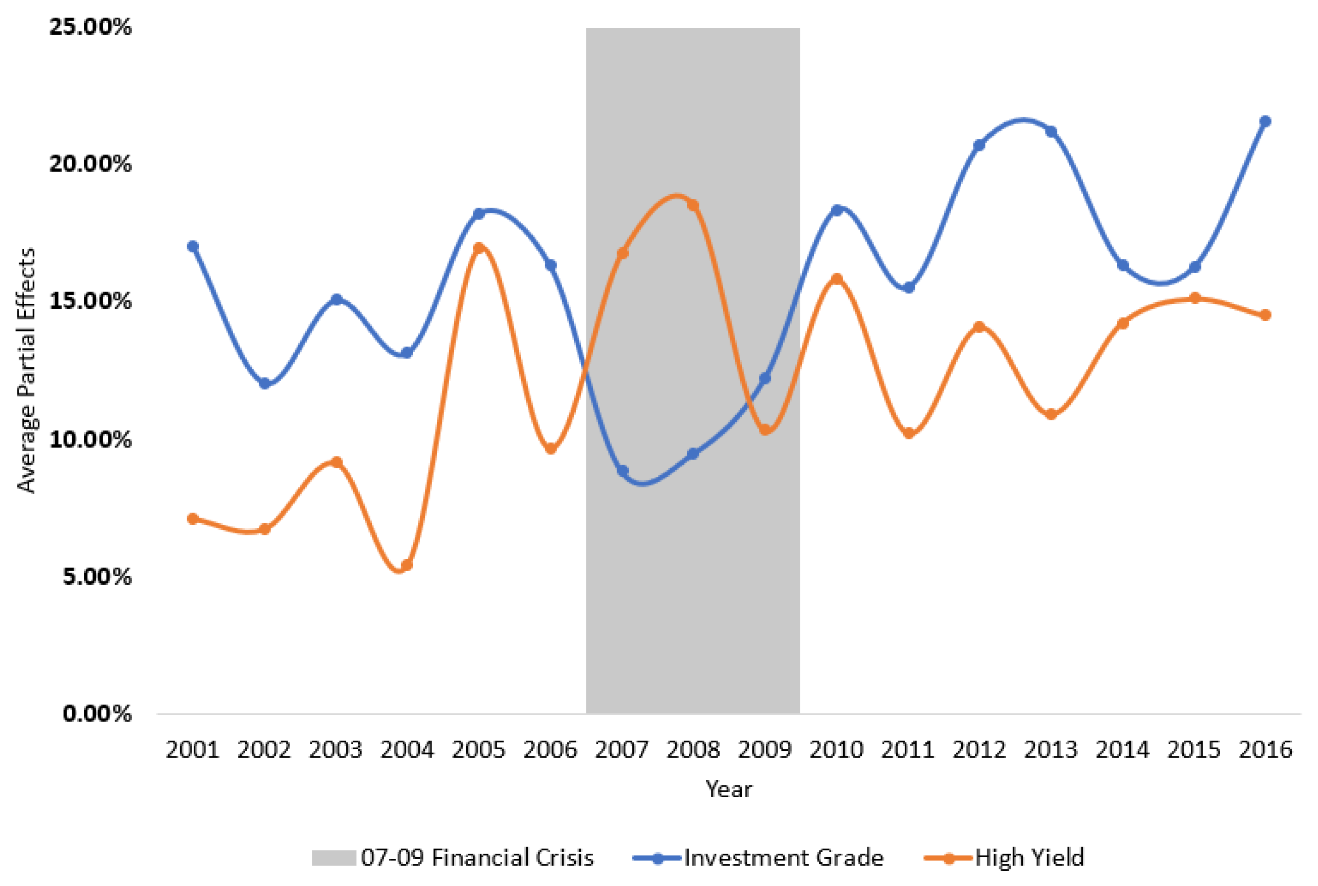
In Figure 4, I report the APE of a one standard deviation change in the MFOI for the investment grade and high yield bonds, respectively. In non-crisis periods, the APE for investment grade bonds was uniformly larger than for high yield bonds, implying that investment grade bonds benefited more from an issuer’s shared-ownership with Moody’s than high yield bonds.

This finding is relatively original in the literature. One possible explanation is related to the “reputation capital” view (Becker and Milbourn 2011; Bolton et al. 2012; White 2002). That is, low quality bonds are more likely to default implying a higher probability of triggering a reputation loss.14 To protect its reputation, Moody’s might be more conservative and apply a more stringent rating standard to low quality bonds.

It is intriguing that this pattern reversed during the 2007–2009 crisis. In 2008, as the MFOI ascends by one standard deviation, high-yield bonds were twice as likely to receive a better rating compared with investment grade bonds (18.5% vs. 9.4%). As can be seen from

Table 3. Distribution of Moody’s Ratings.

	Investment Grade (IG)				High Yield (HY)
Year	Aaa	Aa	A	Baa	Ba	B	C	Total	% of IG
2001	10	45	162	214	111	94	11	647	66.62%
2002	1	78	142	212	71	105	7	616	70.29%
2003	9	112	149	210	123	168	30	801	59.93%
2004	3	81	91	174	89	155	18	611	57.12%
2005	6	118	106	150	86	88	15	569	66.78%
2006	3	164	161	189	58	65	22	662	78.10%
2007	8	238	326	151	48	69	13	853	84.76%
2008	2	110	151	139	29	11	4	446	90.13%
2009	3	35	124	211	88	91	11	563	66.25%
2010	7	51	101	172	90	110	26	557	59.43%
2011	10	35	140	201	41	82	14	523	73.80%
2012	3	41	153	261	83	116	25	682	67.16%
2013	12	49	173	311	95	105	31	776	70.23%
2014	8	32	139	303	92	92	20	686	70.26%
2015	20	28	198	370	78	55	7	756	81.48%
2016	26	59	219	357	80	65	3	809	81.71%
Total	131	1276	2535	3625	1262	1471	257	10,557

, from 2004 to 2008, the proportion of investment grade bonds increased from 57% to 90%. It is in the same period that Moody’s favorable treatment toward high yield bonds nearly quadrupled (from Figure 4, the APE on high-yield bonds increased from 5.4% to 18.5%). As one might intuitively expect, the ratings on some high-yield bonds were perhaps inflated as a result of the growing connection between bond issuers and Moody’s through common shareholders.

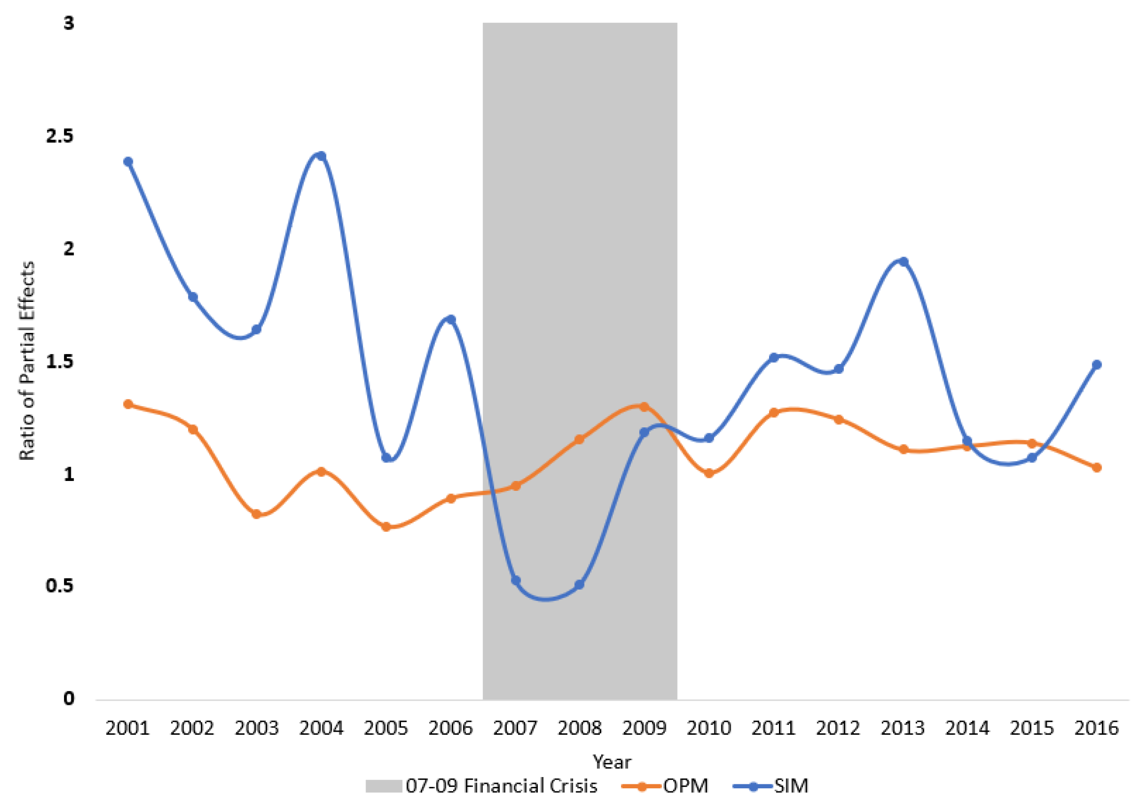
The differences in partial effects across rating categories are often “muted” in a parametric setting. In OPM, rating probabilities for all categories are governed by the same Gaussian cumulative distribution function; such a distribution function, moreover, is roughly linear in the center of its support, making it more challenging to identify the heterogeneous effect across rating categories. As can be seen from Figure 5, the ratio of APE between investment grade and high yield bonds from OPM, as depicted by the yellow-dashed line, remains near unity, implying that the two groups of bonds benefit almost equally from a strengthening shared-ownership relation.

4.3. A Placebo Test for Rating Bias

While a reasonably large set of characteristics were controlled for in the model, and there can be omitted variables that are correlated with the portfolio selection criteria of Moody’s shareholders. After all, institutional shareholders, irrespective of their relationship with Moody’s, tend to invest on firms with higher credit worthiness. As such, the partial effects of the MFOI may only reflect the impact of unobserved characteristics and not necessarily any “rating bias” from Moody’s. To make the analysis more meaningful, I performed a placebo test to check if the bias still existed for bonds related to a portfolio of “false owners” (institutional investors that do not own Moody’s).

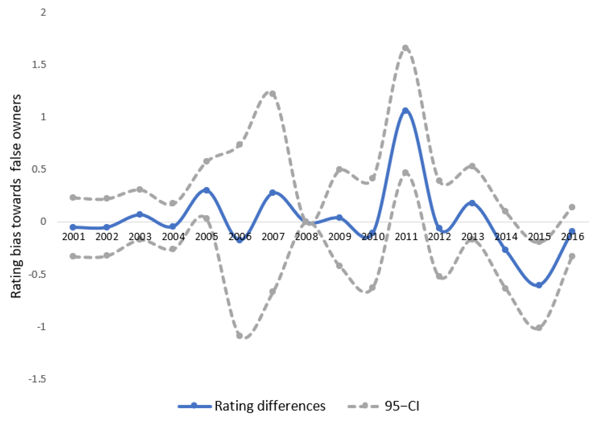
Moody’s ten leading institutional owners are reported in

Table 4. Moody’s major institutional owners from 2001–2016.

Shareholder	T	Mean	Max	Min
HARRIS ASSOCIATES L.P.	21	2.42%	5.02%	0.00%
CHILDREN’S INV MGMT (UK) LLP	20	2.29%	5.31%	0.01%
SANDS CAPITAL MANAGEMENT, INC.	28	3.01%	5.59%	0.40%
T. ROWE PRICE ASSOCIATES, INC.	64	1.47%	5.94%	0.18%
BARCLAYS BANK PLC	55	2.52%	6.32%	0.03%
GOLDMAN SACHS & COMPANY	63	1.94%	7.24%	0.01%
VALUEACT CAPITAL MGMT, L.P.	13	5.19%	7.77%	0.93%
VANGUARD GROUP, INC.	64	3.79%	7.98%	1.64%
MSDW & COMPANY	57	2.20%	8.14%	0.22%
DAVIS SELECTED ADVISERS, L.P.	51	5.56%	8.14%	0.10%
FIDELITY MANAGEMENT & RESEARCH	64	1.99%	9.08%	0.00%
CAPITAL RESEARCH GBL INVESTORS	13	4.80%	11.31%	0.07%
CAPITAL WORLD INVESTORS	35	6.07%	12.60%	0.66%
BERKSHIRE HATHAWAY INC.	64	14.87%	20.43%	11.33%

Note: T = Periods of holding Moody’s stocks (out of 64 quarters).

, most of which are investment/wealth management companies, such as Vanguard and Fidelity. A placebo group was constructed using comparable asset managers that do not own Moody’s stocks. Starting with the fifteen largest asset management companies by AUM, I chose two mangers that do not own Moody’s—Merrill Lynch and BNY Mellon. A dummy variable Placebo was created that takes the value of one for firms who are owned by either firm and zero otherwise. The rating bias, as measured by the rating difference between the two groups, should be zero as the two “false owners” are used. As can be seen from Figure 6, for every year in the sample, except 2011 and 2015, the rating bias remained small and was not statistically different from zero.

4.4. Bias in Issuer Ratings

This paper used bond ratings while the literature also studies issuer ratings. To check whether our empirical results held for issuer ratings, I re-estimated the model for bonds that were “senior-unsecured”—these bonds receive issuer ratings. Note that the bond index in the original model would be redundant in this case because all bonds within the firm receive the same issuer rating. As such, I estimated a double-index model with the firm characteristics and MFOI. The APEs of the MFOI for each year are reported in a similar fashion in Figure 7.

The economic magnitude of the APEs are not identical to those from the three-index model; however, this should not be too surprising because not all firms in the original sample issued senior unsecured bonds. In fact, the sample size decreases substantially from 10,557 to 7485 after focusing only on senior unsecured bonds. Nevertheless, the general patterns of APE are in accord with the three-index model reported in Figure 4. That is, our previous conclusions about the rating bias on bond ratings are likely to extend to issue ratings as well.

5. Conclusions

During the 2007–2009 financial crisis, credit rating agencies (CRAs) were criticized for assigning inflated ratings to mortgage-backed securities and other structured products. A similar phenomenon was documented on other asset classes, such as corporate bonds (Kedia et al. 2017; Strobl and Xia 2012) and CDOs (Griffin and Tang 2012). The relaxed rating standard was largely attributable to conflicts of interest arising out of the CRA’s business model. In this paper, I propose a semiparametric model to investigate to what extent Moody’s ratings are affected by the economic interests of its shareholders, which is pertinent for the regulation of credit rating agencies.

Compared with extant bond rating models, the proposed model has two key features: (i) I explicitly consider the impact of conflicts of interest on ratings through common shareholders, (ii) the model imposes few distributional and functional form restrictions on the underlying rating process. Specifically, explanatory variables enter the model in the form of multiple indices that can interact with each other freely. Asymptotic results of the index parameters estimator are established after several bias corrections. While the focus of this paper is on credit ratings, the estimation and inference framework with multiple-indices can be applied to other contexts.

By estimating the heterogeneous (partial) effects of MFOI, which is a self-constructed index for the degree of shared-ownership connection between Moody’s and bond issuers, I found that high-yield bonds were unlikely to be treated with favoritism. One plausible explanation for this phenomenon is that overrating a subprime bond would incur a greater expected reputation loss than overrating a safe bond.

References

1. Abrevaya, Jason, Yu-Chin Hsu, and Robert Lieli. 2015. Estimating conditional average treatment effects. Journal of Business & Economic Statistics 33: 485–505. [Google Scholar]
2. Ahn, Hyungtaik, Hidehiko Ichimura, James L. Powell, and Paul A. Ruud. 2017. Simple estimators for invertible index models. Journal of Business & Economic Statistics 36: 1–10. [Google Scholar]
3. Amemiya, Takeshi. 1981. Qualitative response models: A survey. Journal of Economic Literature 19: 1483–536. [Google Scholar]
4. Baghai, Ramin P., Henri Servaes, and Ane Tamayo. 2014. Have rating agencies become more conservative? Implications for capital structure and debt pricing. The Journal of Finance 69: 1961–2005. [Google Scholar] [CrossRef]
5. Becker, Bo, and Todd Milbourn. 2011. How did increased competition affect credit ratings? Journal of Financial Economics 101: 493–514. [Google Scholar] [CrossRef]
6. Blundell, Richard W., and James L. Powell. 2004. Endogeneity in semiparametric binary response models. The Review of Economic Studies 71: 655–79. [Google Scholar] [CrossRef]
7. Bolton, Patrick, Xavier Freixas, and Joel Shapiro. 2012. The credit ratings game. The Journal of Finance 67: 85–111. [Google Scholar] [CrossRef]
8. Chen, Xiaohong. 2007. Large sample sieve estimation of semi-nonparametric models. In Handbook of Econometrics. Amsterdam: Elsevier BV, vol. 6, pp. 5549–632. [Google Scholar]
9. Coppejans, Mark. 2007. On efficient estimation of the ordered response model. Journal of Econometrics 137: 577–614. [Google Scholar] [CrossRef]
10. Donkers, Bas, and Marcia Schafgans. 2008. Specification and estimation of semiparametric multiple-index models. Econometric Theory 24: 1584–606. [Google Scholar] [CrossRef]
11. Griffin, John M., and Dragon Yongjun Tang. 2012. Did subjectivity play a role in cdo credit ratings? The Journal of Finance 67: 1293–328. [Google Scholar] [CrossRef]
12. Härdle, Wolfgang, and Thomas M. Stoker. 1989. Investigating smooth multiple regression by the method of average derivatives. Journal of the American Statistical Association 84: 986–95. [Google Scholar] [CrossRef] [Green Version]
13. He, Jie, Jun Qian, and Philip E. Strahan. 2015. Does the market understand rating shopping? predicting mbs losses with initial yields. The Review of Financial Studies 29: 457–85. [Google Scholar] [CrossRef]
14. Horowitz, Joel L. 1998. Semiparametric Methods in Econometrics: Lecture Notes in Statistics. New York: Springer Science & Business Media, vol. 131. [Google Scholar]
15. Horowitz, Joel L., and Wolfgang Härdle. 1996. Direct semiparametric estimation of single-index models with discrete covariates. Journal of the American Statistical Association 91: 1632–40. [Google Scholar] [CrossRef]
16. Ichimura, Hidehiko. 1993. Semiparametric least squares (sls) and weighted sls estimation of single-index models. Journal of Econometrics 58: 71–120. [Google Scholar] [CrossRef] [Green Version]
17. Ichimura, Hidehiko, and Lung-Fei Lee. 1991. Semiparametric least squares estimation of multiple index models: Single equation estimation. In Nonparametric and Semiparametric Methods in Econometrics and Statistics. Paper presented at Fifth International Symposium in Economic Theory and Econometrics, Cambridge, UK, July 26; pp. 3–49. [Google Scholar]
18. Jiang, John Xuefeng, Mary Harris Stanford, and Yuan Xie. 2012. Does it matter who pays for bond ratings? Historical evidence. Journal of Financial Economics 105: 607–21. [Google Scholar] [CrossRef]
19. Kedia, Simi, Shivaram Rajgopal, and Xing Zhou. 2016. Large shareholders and credit ratings. Journal of Financial Economics 124: 632–53. [Google Scholar] [CrossRef]
20. Klein, Roger, and Chan Shen. 2010. Bias corrections in testing and estimating semiparametric, single index models. Econometric Theory 26: 1683–718. [Google Scholar] [CrossRef] [Green Version]
21. Klein, Roger W., and Robert P. Sherman. 2002. Shift restrictions and semiparametric estimation in ordered response models. Econometrica 70: 663–91. [Google Scholar] [CrossRef]
22. Klein, Roger W., and Richard H. Spady. 1993. An efficient semiparametric estimator for binary response models. Econometrica: Journal of the Econometric Society 61: 387–421. [Google Scholar] [CrossRef] [Green Version]
23. Lewbel, Arthur. 2000. Semiparametric qualitative response model estimation with unknown heteroscedasticity or instrumental variables. Journal of Econometrics 97: 145–77. [Google Scholar] [CrossRef]
24. Ma, Xinwei, and Jingshen Wang. 2019. Robust inference using inverse probability weighting. Journal of the American Statistical Association 115: 1–10. [Google Scholar] [CrossRef]
25. Manski, Charles F. 1985. Semiparametric analysis of discrete response: Asymptotic properties of the maximum score estimator. Journal of Econometrics 27: 313–33. [Google Scholar] [CrossRef]
26. Mathis, Jerome, James McAndrews, and Jean-Charles Rochet. 2009. Rating the raters: Are reputation concerns powerful enough to discipline rating agencies? Journal of Monetary Economics 56: 657–74. [Google Scholar] [CrossRef]
27. Powell, James L., James H. Stock, and Thomas M. Stoker. 1989. Semiparametric estimation of index coefficients. Econometrica: Journal of the Econometric Society 57: 1403–430. [Google Scholar] [CrossRef]
28. Sangiorgi, Francesco, Jonathan Sokobin, and Chester Spatt. 2009. Credit-Rating Shopping, Selection and the Equilibrium Structure of Ratings. Technical Report, Working Paper. Pittsburgh: Stockholm School of Economics, Carnegie Mellon University. [Google Scholar]
29. Shen, Chan, and Roger Klein. 2019. Recursive Differencing for Estimating Semiparametric Models. Available online: https://economics.rutgers.edu/downloads-hidden-menu/faculty-cv-s/1824-shen-and-klein-2019/file (accessed on 1 December 2019).
30. Silverman, Bernhard W. 1982. Algorithm as 176: Kernel density estimation using the fast fourier transform. Journal of the Royal Statistical Society Series C (Applied Statistics) 31: 93–99. [Google Scholar] [CrossRef]
31. Skreta, Vasiliki, and Laura Veldkamp. 2009. Ratings shopping and asset complexity: A theory of ratings inflation. Journal of Monetary Economics 56: 678–95. [Google Scholar] [CrossRef] [Green Version]
32. Stewart, Mark B. 2005. A comparison of semiparametric estimators for the ordered response model. Computational Statistics & Data Analysis 49: 555–73. [Google Scholar]
33. Strobl, Günter, and Han Xia. 2012. The Issuer-Pays Rating Model and Ratings Inflation: Evidence from Corporate Credit Ratings. Unpublished Working Paper. Available online: http://efa2011.efa-online.org/fisher.osu.edu/blogs/efa2011/files/APE_8_2.pdf (accessed on 1 December 2019).
34. White, Lawrence J. 2002. The credit rating industry: An industrial organization analysis. In Ratings, Rating Agencies and the Global Financial System. Berlin: Springer, pp. 41–63. [Google Scholar]
35. Xia, Yingcun. 2008. A multiple-index model and dimension reduction. Journal of the American Statistical Association 103: 1631–40. [Google Scholar] [CrossRef]
36. Xia, Yingcun, Howell Tong, W. K. Li, and Li-Xing Zhu. 2002. An adaptive estimation of dimension reduction space. Journal of the Royal Statistical Society Series B Statistical Methodology 64: 363–410. [Google Scholar] [CrossRef]
Figure 1. An illustration.
Econometrics 09 00023 g001
Figure 2. Time series variation in conflicts of interest from 2001–2016.
Econometrics 09 00023 g002
Figure 3. Comparison of the Coefficient Estimates from SIM and OPM.
Econometrics 09 00023 g003
Figure 4. Average partial effects of the MFOI.
Econometrics 09 00023 g004
Figure 5. Ratio of the APE between investment grade and high yield bonds.
Econometrics 09 00023 g005
Figure 6. Placebo test using Merrill Lynch and BNY Mellon as “False Owners”. Note: The rating difference in 2008 is not identified because all 446 bonds are issued by firms related with Merrill Lynch or BNY Mellon.
Econometrics 09 00023 g006
Figure 7. The average partial effects of MFOI (on issuer ratings).
Econometrics 09 00023 g007