Information Flow in Times of Crisis: The Case of the European Banking and Sovereign Sectors

Abstract

Crises in the banking and sovereign debt sectors give rise to heightened financial fragility. Of particular concern is the development of self-fulfilling feedback loops where crisis conditions in one sector are transmitted to the other sector and back again. We use time-varying tests of Granger causality to demonstrate how empirical evidence of connectivity between the banking and sovereign sectors can be detected, and provide an application to the Greek, Irish, Italian, Portuguese and Spanish (GIIPS) countries and Germany over the period 2007 to 2016. While the results provide evidence of domestic feedback loops, the most important finding is that financial fragility is an international problem and cannot be dealt with purely on a country-by-country basis.

1. Introduction

Crisis conditions in the financial sector can be propagated and reinforced by a vicious feedback loop between the banking sector and the sovereign debt sector. The feedback loop relies on two stylized facts: first, banks typically have large holdings of sovereign debt on their balance sheets and, second, when governments bailout an ailing financial sector they fund this by issuing sovereign debt. A feedback loop may result from poor macroeconomic management which reduces the value of sovereign bonds and hence the value of the bank balance sheets. Because this affects bank regulatory capital requirements (sovereign bonds are considered a high quality asset), it will force banks to seek more high-quality capital and/or reduce its lending making economic conditions weaker. This reduces the value of the sovereign debt again, further weakening bank balance sheets. If this mechanism spirals far enough, it will result in a balance sheet induced crises for the banks. The feedback loop may also be established in the opposite direction. If the banking sector comes under stress, for example, by overexposure to mortgage backed securities when housing prices fall, the government may choose to offer a support package to limit the damage. This package, in turn, is financed by the issuance of sovereign debt, which may weaken the value of the stock of sovereign debt. The reduced value of the debt then feeds back to the balance sheets of the banking sector and the loop is established. These feedback loops are described as diabolical loops (Brunnermeier et al. 2016) or doom loops (Fahri and Tirole 2018). Crises involving more than one sector are well known to be vastly more economically costly than those restrained to one market, so there are considerable gains to be made from understanding how they evolve.

The direction and origin of feedback loops is an empirical matter; and recent theory points to the difficulty in identifying the dominant mechanism (Fahri and Tirole 2018). In theory, feedback loops can originate in either the banking or the sovereign sectors. Acemoglu et al. (2015) argue that the source of stress is in the banking sector where debt markets play the role of a safe-haven asset. Acharya et al. (2014), on the other hand, argue that that poor macroeconomic policy choices lead to the need for recapitalizing government funds via sovereign debt issuance and that the origin of the loop is in the sovereign sector. In this case, the stress to banks is not caused by the actions of the bank, but, once new debt is issued, this places further stress on the banks.

Our application focuses on the European markets involved in the crisis conditions prevailing from 2007 onward, comprising credit default spreads (CDS) data from the Greek, Irish, Italian, Portuguese and Spanish (GIIPS) markets and the German market, during the period 2007 to 2016. This sample period includes both the global financial crisis and the European sovereign debt crisis and is well suited to an examination of the vulnerability of the banking and sovereign debt sectors over periods of stress. In particular, the focus is on the flow of information during crisis conditions. In particular, the direction and impact of transmissions from each of the banking and debt markets in these five countries on each other is examined, rather than restricting the analysis to debt and banking sectors in a single country or treating foreign sovereign debt as riskless (see Fahri and Tirole (2018) for a review of existing modelling frameworks). This development is necessary because financial institutions often hold substantial internationally diversified portfolios. The cross-country dimension allows for financial fragility to be propagated both within countries and across countries and for the existence of international feedback loops. In other words, feedback loops may involve large portfolios of internationally diversified sovereign assets held by banking institutions that operate across geographical borders.

The measures of financial vulnerability we compute are based on recent developments in change detection for Granger causality using the rolling window algorithm for possibly integrated vector autoregressive (VAR) systems (Shi et al. 2018a). The algorithm computes all possible direct pairwise Granger causality tests for every rolling window sub-sample. To deal with the problem of multiple tests of the same null hypothesis, a bootstrapping procedure is used to control the overall size of the testing strategy Shi et al. (2018a, 2018b).

In line with the existing literature on systemic risk and contagion in financial crises, only direct causal links are considered (Billio et al. 2012; Dungey et al. 2015), a convention which perhaps reflects the view that these direct links are of first-order importance. This convention has meant that any indirect causal links as defined in Lütkepohl (1993) or Dufour and Renault (1998), in which two variables are connected indirectly through other variables, are usually not explicitly accounted for. The empirical work reported here follows convention and focusses only on direct links. This choice is dictated by the explicit focus of the paper on sub-sampling and changing causal structures, a focus which de-emphasises the existence of a constant model structure in which indirect links are able to be identified reliably. It may be possible for the information on indirect links, as in the Granger causality test of Dufour et al. (2006), to be extracted from the exhaustive set of pairwise one-period-ahead Granger causality analysis conducted in this paper. This avenue of research is however left for future work.

The contribution made by this paper relates to econometric modelling in the sense that a recently-developed econometric method is used in a new and innovative way to address a contemporary question of immense importance, namely, the relationship between the sovereign debt and banking sectors in times of crisis. These new econometric tools are potentially relevant to many policy problems, and our contribution includes the adjustments necessary to move between econometric theory and a sophisticated practical application. Examples of the adjustments include a bootstrap method for assessing the significance of a global information transmission index and also the introduction of signed causal effects to aid interpretation.

While theoretical papers have sought to throw light upon this relationship between the banks and sovereign debt, there is little or no empirical understanding of the nuances of this interplay. It is true to say that sharp empirical results are difficult to come by in an area as complex as the one we address, but we believe that there are four interesting empirical conclusions that emerge from our work. First, not only is information flow between the sectors increases significantly in times of crisis. Moreover, the channels of Granger causality are subject to rapid change over the sample period opening. It is clear that any study attempting to examine longer term relationships between the sectors based on a maintained structure is going to encounter difficulties. Second, although the causal effects are subject to change, these changes admit interpretation in terms of the timeline of important events during the global financial crisis and the sovereign debt crisis in the Eurozone. This correspondence provides a strong empirical vindication of the method, which at this point is relatively untested in the literature. Third, we are able to identify at least four domestic feedback loops in which the crisis is manifest in terms of information flow from one sector to the other, immediately followed by a period of reverse information flow. In three of these four episodes, the prima facie evidence is that the origin of the vulnerability is in the banking sector. Fourth, although feedback loops are easiest to identify in a domestic setting, we provide clear evidence of international connectivity during these crisis periods. The policy implications of this finding are important; it is clear that domestic solutions alone cannot be effective. Of course, we cannot provide actual policy prescriptions based on these results, but the general message is nonetheless an important one.

The rest of the paper is organized as follows. Section 2 develops a simple illustrative model which is used to define all the information measures proposed to capture transmission of crises between markets. Section 3 outlines the algorithms for assessing time-varying Granger causality together with a bootstrap procedure designed to deal with inference in the presence of multiple tests of the same hypothesis. The data are described in Section 4. Section 5, Section 6 and Section 7 are the main econometric results. A global view of the causal network is provided in Section 5, Section 6 investigates linkages within each sector and Section 7 considers the evidence for feedback loops formed within single countries and the international linkages across sectors. Section 8 provides brief conclusions.

2. Modelling Financial Linkages

Let ${\mathbf{x}}_t$ and ${\mathbf{y}}_t$ represent credit risk in the sovereign debt and the banking sectors, respectively. VAR models are commonly used in the existing systemic risk literature to measure connectivity between variables (Billio et al. 2012). As an illustration of the concepts, we consider a VAR(1) with $s=3$ countries, so that ${\mathbf{x}}_t=[x_{1t},x_{2t},x_{3t}]$ and ${\mathbf{y}}_t=[y_{1t},y_{2t},y_{3t}]$. In this case, the model is

$$\begin{array}{cc}\hfill \left[\begin{array}{c}{x}_{1t}\\ x_{2t}\\ x_{3t}\\ y_{1t}\\ y_{2t}\\ y_{3t}\end{array}\right]& =\left[\begin{array}{c}{z}_{1t}\\ z_{2t}\\ z_{3t}\\ z_{4t}\\ z_{5t}\\ z_{6t}\end{array}\right]=\left[\begin{array}{cccccc}{\pi }_{11}& {\pi }_{12}& {\pi }_{13}& {\pi }_{14}& {\pi }_{15}& {\pi }_{16}\\ {\pi }_{21}& {\pi }_{22}& {\pi }_{23}& {\pi }_{24}& {\pi }_{25}& {\pi }_{26}\\ {\pi }_{31}& {\pi }_{32}& {\pi }_{33}& {\pi }_{34}& {\pi }_{35}& {\pi }_{36}\\ {\pi }_{41}& {\pi }_{42}& {\pi }_{43}& {\pi }_{44}& {\pi }_{45}& {\pi }_{46}\\ {\pi }_{51}& {\pi }_{52}& {\pi }_{53}& {\pi }_{54}& {\pi }_{55}& {\pi }_{56}\\ {\pi }_{61}& {\pi }_{62}& {\pi }_{63}& {\pi }_{64}& {\pi }_{65}& {\pi }_{66}\end{array}\right]\left[\begin{array}{c}{z}_{1t-1}\\ z_{2t-1}\\ z_{3t-1}\\ z_{4t-1}\\ z_{5t-1}\\ z_{6t-1}\end{array}\right]+\left[\begin{array}{c}{\epsilon }_{1t}\\ {\epsilon }_{2t}\\ {\epsilon }_{3t}\\ {\epsilon }_{4t}\\ {\epsilon }_{5t}\\ {\epsilon }_{6t}\end{array}\right],\hfill \end{array}$$

(1)

where ${\epsilon }_{it}$ (with $i=1,\cdots 6$) are the error terms.

This simple model accounts for all the potential linkages between sectors within a country as well as across countries. For example, ${\pi }_{12}$ represents the Granger causality effect from country 2 to country 1 in the sovereign debt sector, while ${\pi }_{25}$ represents the effect of the banking sector in country 2 on sovereign debt in country 2. The autoregressive processes given by the diagonal elements ${\pi }_{ii}$ are not of interest in our problem.

The method adopted here is to test for Granger causality (Granger 1969) systematically between all possible pairs of variables. Suppose the maximum order of integration of the illustrative VAR system is unity. To take care of the non-stationarity in the system, Dolado and Lütkepohl (1996) and Toda and Yamamoto (1995) suggest using a lag augmented VAR system such that

$${\mathbf{z}}_{\mathbf{t}}=\Pi {\mathbf{z}}_{t-1}+\Phi {\mathbf{z}}_{t-2}+{\epsilon }_t,$$

(2)

where ${\mathbf{z}}_t={[x_{1t},x_{2t},x_{3t},y_{1t},y_{2t},y_{3t}]}^{\prime }$, $\Pi$ is the first order autoregressive coefficient in Label (1), $\Phi {\mathbf{z}}_{t-2}$ is the augmented term with $\Phi$ being a zero matrix under the DGP of (1), and ${\epsilon }_t={[{\epsilon }_{1t},{\epsilon }_{2t},{\epsilon }_{3t},{\epsilon }_{4t},{\epsilon }_{5t},{\epsilon }_{6t}]}^{\prime }$.

The null hypothesis of the test for a causal influence from $z_j$ to $z_i$ is $H_0:{\pi }_{ij}=0$. The Wald test statistic ${\mathcal{W}}_{j\to i}$ is obtained by estimating the unrestricted VAR model (2). All the pairwise Granger causality tests require testing zero restrictions on all the off-diagonal elements of the matrix with elements ${\pi }_{ij}$ so that there will be $n(n-1)$ Wald test statistics, with $n=2s=6$ in this instance. Of course, in higher order VAR models, the test of Granger causality will involve zero restrictions on the higher-order lags as well, but even in VAR(p) models the number of actual pairs to be tested remains constant at $n(n-1)$. These statistics are now used in a number of different ways to summarize the linkages.

2.1. A Global Summary Measure

Let $I_{j\to i}$ be a dummy variable, taking value one if the p-value of the $W_{j\to i}$ is less than $10\%$. The percentage of significant Granger causality relationships among all possible links is denoted by ${\mathcal{P}}_{\mathbf{z}}$ and defined as

$$\begin{array}{cc}\hfill {\mathcal{P}}_{\mathbf{z}}& =\frac{1}{n(n-1)}\sum _{i=1}^n\sum _{j=1,i\ne j}^n{I}_{j\to i}.\hfill \end{array}$$

(3)

This index calculates the average information flow across all possible links and can be interpreted as a measure of market uncertainty. It will take the value 1 when the information flow is at maximum capacity, which may be interpreted as a situation of greatest uncertainty.1

Under the null hypothesis of no information flow within the system (i.e., no Granger causality between any pair of the variables), the causal indicators $I_{j\to i}$ are independent and hence by the Central Limit Theorem

$${\mathcal{P}}_{\mathbf{z}}\stackrel{d}{⟶}N\left({\displaystyle p,\frac{p(1-p)}{n(n-1)}}\right),$$

(4)

as $n\to \infty$, with p being the probability of making false positive conclusions of the Granger causality test.

2.2. Local Summary Measures

The local summary measures which we use in this paper are constructed by considering special cases of interest that limit the number of terms included in the summations defined in Equation (3). We examine the local linkages along two dimensions: linkages within sectors and linkages between sectors.

(a) Within sectors

Linkages within the sovereign sector are the causal relationships between the variables ${\mathbf{x}}_t=[x_{1t},x_{2t},x_{3t}]$ (or $z_{1t}$, $z_{2t}$ and $z_{3t}$ using the more general notation). We consider causal relationships from the sovereign sector in country i to the sovereign sectors in all other countries (referred to as S2S*) and from the banking sector in country i to all other banking sectors (referred to as B2B*). The indicators for the significance of at least one link from the sovereign sector in country i to a sovereign sector located elsewhere and from the banking sector in country i to a banking sector elsewhere are denoted by $I_{S2S*,i}$ and $I_{B2B*,i}$, respectively. Taking country 1 in the illustrative model as an example, they are defined as

$$\begin{array}{c}\hfill \begin{array}{cc}\hfill I_{S2S*,1}=1(I_{1\to 2}=1\mathrm{or}{I}_{1\to 3}=1)& \mathrm{from}\mathrm{Country}1\mathrm{S}2\mathrm{S}*,\hfill \\ \hfill I_{B2B*,1}=1(I_{4\to 5}=1\mathrm{or}{I}_{4\to 6}=1)& \mathrm{from}\mathrm{Country}1\mathrm{B}2\mathrm{B}*,\hfill \end{array}\end{array}$$

(5)

where $1(.)$ is an indicator function, taking value one if the argument is true and zero otherwise.

(b) Between sectors

The between sectors links can be further divided into two categories: within country and across countries. We refer to the causality from the sovereign sector to the banking sector within a country as S2B and vice-versa as B2S. Let $I_{S2B,i}$ and $I_{B2S,i}$ be the indicators of the two Granger causal relationships in country i, taking value one when significant and zero otherwise. There are six possible cases (two for each country). For example,

$$\begin{array}{cc}{I}_{S2B,1}\equiv I_{1\to 4}& \mathrm{S}2\mathrm{B}\mathrm{in}\mathrm{Country}1,\\ I_{B2S,1}\equiv I_{4\to 1}& \mathrm{B}2\mathrm{S}\mathrm{in}\mathrm{Country}1.\end{array}$$

(6)

We also consider causal relationships from the sovereign sector in country i to the banking sectors in all other countries (referred to as S2B*) and from the banking sector in country i to the sovereign sectors in all other countries (referred to as B2S*). The indicators for the significance of at least one link from the sovereign sector in country i to a banking sector located elsewhere and from the banking sector in country i to a sovereign sector located elsewhere are denoted by $I_{S2B*,i}$ and $I_{B2S*,i}$, respectively. The indicators for country 1 are defined as

$$\begin{array}{c}\hfill \begin{array}{cc}\hfill I_{S2B*,1}=1(I_{1\to 5}=1\mathrm{or}{I}_{1\to 6}=1)& \mathrm{from}\mathrm{Country}1\mathrm{S}2\mathrm{B}*,\hfill \\ \hfill I_{B2S*,1}=1(I_{4\to 2}=1\mathrm{or}{I}_{4\to 3}=1)& \mathrm{from}\mathrm{Country}1\mathrm{B}2\mathrm{S}*.\hfill \end{array}\end{array}$$

(7)

The difference between the indicators defined in Labels (6) and (5) reveals the importance of the between sector across country links.

2.3. Signed Effects

By construction, the Wald test of the null hypothesis of no Granger causality is a chi-squared deviate and is therefore positive. Using the information in this way suppresses the sign of the linkage. To provide further information on causal linkages, we compute a signed transmission index, denoted by ${\mathcal{R}}_{j\to i}$ for the causality from variable $z_j$ to $z_i$. This index provides an indication of the direction of influence (positive or negative) from $z_j$ to $z_i$. As in the case of the Granger causality tests, there will be $n(n-1)$ numbers of $R_{j\to i}$ indexes.

In the general VAR(p) case, the ${\mathcal{R}}_{j\to i}$ index is defined as the summation of the (heteroskedastic consistent) t-statistics of all the lagged coefficients of variable $z_j$ in the equation for $z_i$, i.e., the t-statistics of the constituent elements of the associated Granger causality test from $z_j$ to $z_i$. For the illustrative model (with only one lag), ${\mathcal{R}}_{j\to i}$ is the t-statistic of the coefficient ${\pi }_{ij}$ such that

$${\mathcal{R}}_{j\to i}=\frac{{\widehat{\pi }}_{ij}}{\mathrm{se}\left({\widehat{\pi }}_{ij}\right)},$$

(8)

where $\mathrm{se}(.)$ is the heteroskedastic consistent standard error of the estimator. Therefore, the signed index follows a t-distribution under the null. The limiting distribution of the ${\mathcal{R}}_{j\to i}$ index for the general case will depend on the correlation structure among the lagged coefficients.

We further calculate the averaged signed effect for within sector transmission and and the averaged signed effect for between sectors across country transmission. Taking country 1 as an example, the averaged signed effect for within sector transmission is defined as

$$\begin{array}{c}\hfill \begin{array}{cc}\hfill {\overline{\mathcal{R}}}_{S2S\ast ,1}=\frac{1}{2}({\mathcal{R}}_{1\to 2}+{\mathcal{R}}_{1\to 3})& \mathrm{from}\mathrm{Country}1\mathrm{S}2\mathrm{S}*,\hfill \\ \hfill {\overline{\mathcal{R}}}_{B2B\ast ,1}=\frac{1}{2}({\mathcal{R}}_{4\to 5}+{\mathcal{R}}_{4\to 6})& \mathrm{from}\mathrm{Country}1\mathrm{B}2\mathrm{B}*,\hfill \end{array}\end{array}$$

(9)

and the averaged signed effect for between sector across country transmission is

$$\begin{array}{c}\hfill \begin{array}{cc}\hfill {\overline{\mathcal{R}}}_{S2B\ast ,1}=\frac{1}{2}({\mathcal{R}}_{1\to 5}+{\mathcal{R}}_{1\to 6})& \mathrm{from}\mathrm{Country}1\mathrm{S}2\mathrm{B}*,\hfill \\ \hfill {\overline{\mathcal{R}}}_{B2S\ast ,1}=\frac{1}{2}({\mathcal{R}}_{4\to 2}+{\mathcal{R}}_{4\to 3})& \mathrm{from}\mathrm{Country}1\mathrm{B}2\mathrm{S}*.\hfill \end{array}\end{array}$$

(10)

The limiting distributions of all the average signed indexes outlined here would be an interesting line of inquiry. As this problem would involve substantive additional investigation, it is left for future work.

3. Time Variation and the Multiplicity Issue

Having illustrated the main ideas of the methodology in the simplest possible model, the model is now generalized to allow for more than three countries, more than one lag in the VAR, and also for time variation in the linkages due to changing global financial conditions. Although the ideas are exactly the same as for the simple model, the notation must be modified slightly to reflect the additional complexity of the model.

3.1. Time-Varying Tests of Granger Causality

Once again, let ${\mathbf{x}}_t$ and ${\mathbf{y}}_t$ represent credit risk in the sovereign debt and the banking sectors, respectively. These two variables are now observed in multiple countries so that ${\mathbf{x}}_t=[x_{1t},x_{2t},\cdots ,x_{st}]$ and ${\mathbf{y}}_t=[y_{1t},y_{2t},\cdots ,y_{st}]$, where s is the total number of countries. The lag augmented VAR model, which has a maximum order of integration d,2 is

$${\mathbf{z}}_t=\Pi {\mathbf{z}}_{t,A}^{-}+\Phi {\mathbf{z}}_{t,B}^{-}+{\epsilon }_t$$

(11)

in which ${\mathbf{z}}_t=[{\mathbf{y}}_t,{\mathbf{x}}_t]$, ${\mathbf{z}}_{t,A}^{-}={[1,{\mathbf{z}}_{t-1},{\mathbf{z}}_{t-2},\cdots ,{\mathbf{z}}_{t-k}]}^{\prime }$, ${\mathbf{z}}_{t,B}^{-}={[{\mathbf{z}}_{t-k-1},,\cdots ,{\mathbf{z}}_{t-k-d}]}^{\prime }$, and $\Phi$ equals zero. The dimension of ${\mathbf{z}}_t$ is $n=2s$. The error term ${\epsilon }_t$ is assumed to be an iid sequence of $n-$dimensional random vectors with mean zero and variance ${\Sigma }_{\epsilon }>0$ such that $E|{\epsilon }_{it}{|}^{2+\delta }<\infty$ for some $\delta >0$. This assumption can be further relaxed to allow for conditional heteroskedasticity of unknown forms as in Shi et al. (2018b). In this general model, the test of causality from $z_j$ to $z_i$ will involve taking account of the first k lags of $z_j$.

For the rolling window procedure Swanson (1998); Shi et al. (2018a, 2018b), the ending point of the VAR regression is fixed on the observation of interest t. The starting point of the regression retains a fixed distance from t given by $t_w$, with the latter being the fixed regression window size. Let ${\widehat{\mathbf{ß}}}_t\equiv \mathrm{vec}\left({\widehat{\Pi }}_t\right)$ where ${\widehat{\Pi }}_t$ is the ordinary least squares estimate of $\Pi$ using a sample running from $t-t_w$ to t. Furthermore, define ${\widehat{\Omega }}_t=t_w^{-1}{\sum }_{t=t_1}^t{\widehat{″}}_t{\widehat{″}}_t^{\prime }$ with ${\widehat{″}}_t={\mathbf{z}}_t-{\widehat{\Pi }}_t{\mathbf{z}}_{t,A}^{-}-{\widehat{\Phi }}_t{\mathbf{z}}_{t,B}^{-}$ and ${\mathbf{z}}_t^{-}={[{\mathbf{z}}_{t,A}^{{-}^{\prime }},{\mathbf{z}}_{t,B}^{{-}^{\prime }}]}^{\prime }$. The heteroskedasticity consistent Wald statistic for no causality running from variable $z_j$ to $z_i$ is denoted by ${\mathcal{W}}_{j\to i}\left(t\right)$ and defined as (Shi et al. 2018a)

$${\mathcal{W}}_{j\to i}\left(t\right)=t_w{\left({\mathbf{R}}_{ji}{\widehat{\mathbf{ß}}}_t\right)}^{\prime }{\left[{\mathbf{R}}_{ji}\left({\widehat{\mathbf{V}}}_t^{-1}{\widehat{\mathbf{W}}}_t{\widehat{\mathbf{V}}}_t^{-1}\right){\mathbf{R}}_{ji}^{\prime }\right]}^{-1}\left({\mathbf{R}}_{ji}{\widehat{\mathbf{ß}}}_t\right),$$

(12)

where ${\mathbf{R}}_{ji}$ is a $k\times n(nk+1)$ restriction matrix for the Granger causality running from $z_j$ to $z_i$, ${\widehat{\mathbf{V}}}_t={\mathbf{I}}_n\otimes {\widehat{\mathbf{Q}}}_t$ with ${\widehat{\mathbf{Q}}}_t=\frac{1}{t_w}{\sum }_{t=t_1}^t{\mathbf{z}}_t^{-}{\mathbf{z}}_t^{-\prime }$, and ${\widehat{\mathbf{W}}}_t=\frac{1}{t_w}{\sum }_{t=t_1}^t{\widehat{\xi }}_t{\widehat{\xi }}_t^{\prime }$ with ${\widehat{\xi }}_t={\widehat{″}}_t\otimes {\mathbf{z}}_t^{-}$.

The test statistic has a limiting distribution (Shi et al. 2018a) of

$${\mathcal{W}}_{j\to i}\left(r\right)\Rightarrow {\left[\frac{W_d\left(r\right)-W_d\left(r-r_w\right)}{r_w^{1/2}}\right]}^{\prime }\left[\frac{W_d\left(r\right)-W_d\left(r-r_w\right)}{r_w^{1/2}}\right],$$

(13)

where r and $r_w$ are the fractional counterparts of t and $t_w$, $W_d$ is vector Brownian motion with co-variance matrix ${\mathbf{I}}_d$, and d is the number of restrictions (the rank of $\mathbf{R}$) under the null.

3.2. Multiplicity

In empirical applications, the sub-sample Wald test is conducted for each observation from $t_w$ to T. The total number of tests conducted is $T-t_w+1$. It is well known in the literature that the probability of making a false positive conclusion (i.e., size) rises with the number of hypotheses tested, referred to as the multiplicity issue. Shi et al. (2018a) propose a bootstrap approach to address this issue. Extensive simulations conducted in Shi et al. (2018a) show the attractive empirical performance of the rolling window Granger causality test, in terms of size and power.

The bootstrap algorithm is described here in the context of a bi-variate VAR(1), but the procedure is easily extended to higher dimensional systems. Let $t_b$ be the number of observations in the window over which size is to be controlled. The bootstrap procedure allows the probability of having at least one false positive detection over the sample period $t_b$ to be $5\%$.

Step 1: 

Estimate a bivariate VAR(1) model which imposes the null hypothesis of no Granger causality from $y_2$ to $y_1$ using the full sample. The resultant equation is

$$\left[\begin{array}{c}{x}_t\\ y_t\end{array}\right]=\left[\begin{array}{cc}{\widehat{\varphi }}_{11}& 0\\ {\widehat{\varphi }}_{12}& {\widehat{\varphi }}_{22}\end{array}\right]\left[\begin{array}{c}{x}_{t-1}\\ y_{t-1}\end{array}\right]+\left[\begin{array}{c}{e}_{1t}\\ e_{2t}\end{array}\right]$$

(14)

in which $e_{1t}$ and $e_{2t}$ are the estimated residuals.

Step 2: 

Generate a bootstrap sample with sample size $t_w+t_b-1$

$$\left[\begin{array}{c}{x}_t^b\\ y_t^b\end{array}\right]=\left[\begin{array}{cc}{\widehat{\varphi }}_{11}& 0\\ {\widehat{\varphi }}_{12}& {\widehat{\varphi }}_{22}\end{array}\right]\left[\begin{array}{c}{x}_{t-1}^b\\ y_{t-1}^b\end{array}\right]+\left[\begin{array}{c}{e}_{1t}^b\\ e_{2t}^b\end{array}\right]$$

(15)

where initial values $x_1^b=x_1$ and $y_1^b=y_1$ and the residuals $e_{1t}^b$ and $e_{2t}^b$ are randomly drawn with replacement from the estimated residuals in Step 1.

Step 3: 

Compute the test statistic sequences from the bootstrapped series ${\left\{{\mathcal{W}}_{j\to i}\left(t\right)\right\}}_{t=t_w}^{t_w+t_b-1}$ and the associated maximum values of the test statistic sequences

$${\mathcal{M}}_{j\to i}^b=\underset{t\in [t_w,t_w+{\tau }_b-1]}{max}\left({\mathcal{W}}_{j\to i}\left(t\right)\right).$$

Step 4: 

Repeat Steps 2–3 for $B=499$ times.

Step 5: 

The critical value of the procedure is given by the $95\%$ percentiles of the ${\left\{{\mathcal{M}}_{j\to i}^b\right\}}_{b=1}^B$ sequence.

3.3. Distribution of the Global Transmission Index

Within this rolling window testing framework, the computation of the global summary measure within each window is as outlined previously. The percentage of significant causal links among all possible links at time t, ${\mathcal{P}}_{\mathbf{z}}\left(t\right)$, is computed as

$$\begin{array}{cc}\hfill {\mathcal{P}}_{\mathbf{z}}\left(t\right)& =\frac{1}{n(n-1)}\sum _{i=1}^n\sum _{j=1,i\ne j}^n{I}_{j\to i}\left(t\right),\hfill \end{array}$$

(16)

where $I_{j\to i}\left(t\right)$ is a dummy variable, taking value one if the p-value of the causality test from j to i at time t goes below the cut-off value of $10\%$. The explicit dependence of the index on time t emphasizes that the measure is recomputed for every rolling window. The local summary measures and the signed indexes are also identical to those reported earlier, except that each measure is now computed for each of the windows in the rolling window estimation procedure.

The validity of the Central Limit Theorem governing the asymptotic distribution of ${\mathcal{P}}_{\mathbf{z}}\left(t\right)$ given in Label (4) is unlikely to be a good approximation of the finite sample distribution given that n is small. Furthermore, since the bootstrapping procedure controls the family wise error rate to be 10% over a one-year period, the probability, p, of drawing a false positive conclusion at each time period is less than 10% but unknown. As a consequence, the limiting distribution of the global index cannot be relied upon for statistical inference. As an alternative, a bootstrapped critical value for the index is proposed. Under the null hypothesis, there is no information flow within the system and hence each variable is related only to its own history. The restricted VAR(1) model is estimated with the full sample and bootstrapped samples (with sample size $t_w$) are generated using the estimated coefficients and residuals. The Granger causality test for all possible pairs are conducted on the bootstrapped samples and the global transmission index is calculated. Notice that the sample size of the bootstrapped series equals the minimum window size and hence the Granger causality tests (12) are implemented only for the observation $t=t_w$. This process is repeated 1000 times and the 90% percentile of the global index is taken as the critical value. To reduce computational load, we use the asymptotic critical value for the Granger causality test in the bootstrapping procedure for the global index but with a slight twist. Specifically, we obtain $t_b$ random realizations from the chi-square distribution and calculate the maximum value for the $t_b$ realizations. This process is then repeated 1000 times. We take the 90% percentile of the maximum values as the critical value of the rolling window Granger causality test.

4. Data

The empirical work in this paper uses data for 5-year credit default swap (CDS) spreads as liquid proxies for credit risk; see also Pan and Singleton (2008), Duca and Peltonen (2013), Kalbaskaa and Gatkowskib (2012), Billio et al. (2017). The CDS is a financial swap agreement that the buyer in the CDS contract (usually the creditor of the reference loan) pays a periodic fee to the seller until the contract matures or a credit event occurs. In the event of a loan default or other credit event, the CDS seller compensates the buyer with the difference between the market value and face value of the issue. The `restructuring clause’ of a CDS contract specifies the credit events that trigger settlement.

The data are for Portugal, Ireland, Greece, Italy and Spain (the GIIPS countries), which are the five EU member states that were unable to refinance their government debt or to bail-out over-indebted banks on their own during the debt crisis. The German CDS contract is used as a benchmark. The daily CDS spreads, for the period 27 April 2006 to 8 July 2016, are sourced from the Markit database, as an average across all quotes provided by market makers after a series of data cleaning tests. We focus on the spreads of all the CDS contracts (denominated in US dollars) with a modified-modified restructuring clause for bank CDS and the full restructuring clause for the sovereign CDS.3

We construct a bank CDS spread for each country as the equally weighted portfolio of major banks whose headquarters are in that country.4 The banks are selected according to their total assets and subject to availability of data from Markit. The banks used in this application are listed in

Table 1. List of the banks included in the data sample in each of the GIIPS countries and also Germany as the benchmark.

Country	Bank Name	Country	Bank Name
Greece	EUROBANK ERGASIAS SA	Ireland	ALLIED IRISH BKS PLC
	NAT BK OF GREECE SA		THE GOVERNOR AND CO BOI
			PERMANENT SB PUB LTD CO
Portugal	CAIXA GERAL DE DEPOSITOS SA	Italy	UNI CREDIT
	BANCO ESPIRITO SANTO SA		INTESA SANPAOLO SPA
	BANCO COM PORT		BANCA PASCHI
	BCO BPI SA		BANCO POP SOCO
Germany	DEUTSCHE BANK AG	Spain	BANCO SANTANDER, SA
	COMMERZBANK AG		BBV ARGENTARIA SA
	DZ BK AG		BANKIA SA
	UNICREDIT BANK AG		BANOCO DE SABADELL
	LB BADENWUERTTEMBERG		BANCO POPULAR ESPANOL
	BAYERISCHE LANDESBK
	NORD-LB-GIRO

.

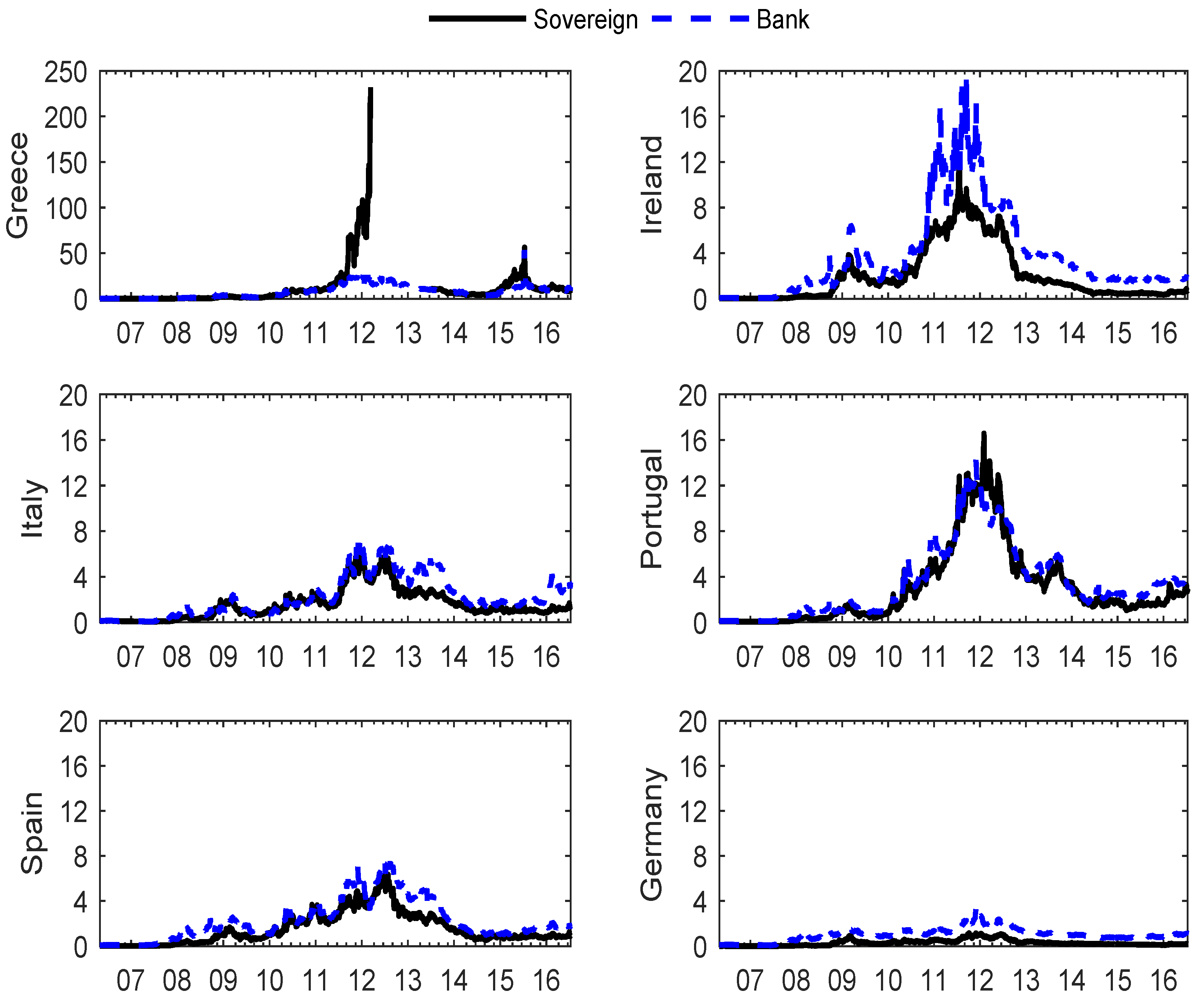
The sovereign and bank CDS spreads are presented in Figure 1. The scale of the problems in Greece is evident in the size of the CDS spread at the peak of the European debt crisis, which is more than ten times that of other countries. The German CDS spread is the lowest during the sample period. Both the sovereign and bank premiums are almost negligible at the beginning of the sample period but rise gradually after late 2007 for all countries.

Following the bailout announcement of the Irish government on 30 September 2008, the CDS premiums of the GIIPS countries deviated from the German CDS, peaking in January 2009. Dungey and Renault (2018) explore contagion between the sovereign CDS spreads for these countries and support the necessity of capturing the behavior of the German CDS and other markets with separate factors at this time.

The CDS spreads of the GIIPS countries began to increase after the Greek government announced a 300 billion Euro debt on 10 December 2009, and the spreads of all countries achieved their historical peak between 2011 and 2012. The default on Greek debt in March 2012 resulted in an abrupt increase of the Greek CDS spread to over 200 basis points, and a subsequent market closure. It was reopened in April 2013 with a premium of around ten basis points, followed by another small bump in the first half of 2015 triggered by the economic recession in the last quarter of 2014.

Portugal and Ireland have the next two largest CDS spreads in the sample. The CDS spreads of Spain and Italy follow each other closely, with some mild deviations in trajectory. The debt crisis increased in late 2011 in Italy and in the second half of 2012 in Spain. The sovereign CDS premiums of the GIIPS countries (except Greece) reached a plateau in mid-2014 and were relatively stable after that.

The bank indices of CDS spreads are generally higher than those for sovereign debt. The bank indices increased steadily from the onset of the global disruptions evident first in the UK in 2007. The upward trend remained in 2008 but with higher volatility. The bank indices dropped after governments announced rescue packages for the financial sector, particularly those after the failure of Lehman Bros in September 2008. A consequence of these support packages was a rapid increase in the sovereign debt risk index. The bank CDS spreads reached their peak during the European debt crisis in late 2009, and subsequently fell, again consistent with the government rescue packages. The bank CDS spreads in Portugal, Spain, and Italy rose again in late 2015 during the 2015–2016 stock market crash. For Greece, both the sovereign and bank indices spiked in May 2015, when the IMF took a hard line on aid as the Greek budget surplus turned to a deficit. Germany, which provided much of the leadership around the European crisis, also experienced a rise in risk indices, but, reflecting its role as an anchor for the Eurozone region, these increases were of a much lower magnitude.

To investigate information flow within and between the sovereign and banking sectors and across countries, we implement the VAR framework, outlined in Section 2, in a multi-country setting use CDS data and construct measures of vulnerability based on tests of Granger causality. The variables ${\mathbf{x}}_t$ and ${\mathbf{y}}_t$ are the 5-year CDS spreads for the sovereign and banking sectors. The modelling framework requires a choice of window size, which we choose to be 260 days or approximately one trading year. The choice here is simply based on the assertion that a year provides a reasonable balance between maintaining sufficient degrees of freedom while also allowing sufficient flexibility to detect changes. The VAR lag order is selected using the Hannan–Quinn information criteria based on a maximum of 20. The selected lag order is 3. Dungey et al. (2017) find that the CDS spreads used in this paper have one unit root and for this reason we choose the maximum order of integration to be one (i.e., $d=1$) and hence the lag augmented VAR is estimated using 4 lags in total. We apply the same lag order for each sub-sample regression.5 For this empirical application, we use a residual bootstrap with 499 replications to obtain the finite sample distributions of the test statistics. Due to the closure of the Greek sovereign market and the need to restart the rolling window process, test results for the period running from 12 March 2012 to 5 June 2014 are not available.

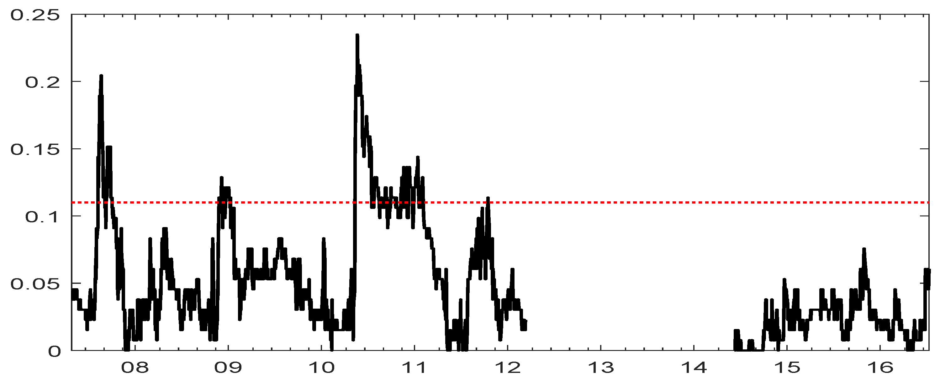
5. A Global View of Linkages

The global transmission index, ${\mathcal{P}}_{\mathbf{z}}\left(t\right)$ given in Equation (16) is plotted in Figure 2 for all possible windows, t. The horizontal dashed line is the 10% critical value for the significance of the global index (i.e., $0.11$) obtained from the procedure outlined in Section 3.3. The null hypothesis of no information flow within the system is rejected when the index exceeds the critical value. The results indicate that the banking and sovereign sectors in these countries were strongly connected during the sub-prime and the European debt crisis periods.

Specifically, the unfolding sub-prime crisis of 2007, involving portfolio problems in Bear Sterns, Freddie Mac, Fanny Mae, BNP Paribus and culminating in Northern Rock requesting emergency funding from the Bank of England in September of that year, is associated with the early period of increased information flow in the European financial system. Interestingly, the Lehman Brothers collapse does not seem to register in terms of this index; a substantial increase in the index occurs in September 2008, but it is not statistically significant. By contrast, the jump in the index in January 2009, when US stock markets plunged in value on expectations of harsh future economic conditions, is significant. Overall, it seems reasonable to conclude that the global index is largely a leading indicator of the crisis in the banking sector.

There is a marked increase in the value of the index in late 2009 corresponding to the substantial revision of the Greece public deficit and the downgrading of Greek debt to BBB by Fitch, although this upward movement is not statistically significant in terms of the bootstrapped critical value. There is no doubt, however, about the significance of the index when Greece and Portugal asked for help from the European Union in April of 2009. The significance of the European debt crisis only begins to drop in terms of measured vulnerability after May 2010 when the European Financial Stability Facility was enacted. The index rises again at the end of 2010 and early 2011, and is particularly evident at the time when Ireland sought help from the European Union in November 2010. The events leading up to the second rescue package for Greece in February 2012, the closure of the Greek sovereign market, and Spain’s request for assistance from the European Union (June 2012) do not register as statistically significant values of the global information index. Thus, once more, it is reasonable to posit that the index is a leading indicator, a conjecture that is consistent with the idea of Granger causality as predictability.

The periods of significance indicated by the global transmission index receive qualified support from empirical evidence obtained using the bubble-detection procedure of Phillips and Shi (2017); Phillips et al. (2015a, 2015b).6 As in Phillips and Shi (2017), the bubble-detection algorithm was applied to the CDS spreads between the GIIPS countries and Germany. The results identify three broad periods of heightened risk in both sovereign and bank sectors (late 2007 to early 2009, early 2010 to early 2012, and 2014 to mid-2015).

The sheer volume of information provided by the time-varying nature of the Granger causality tests provides challenges for both interpretation and presentation. To reveal the importance of each causal link, we calculate the average percentage of significant test statistics over the rolling windows for all possible pairwise causal links. This enables us to focus our attention on the causal links that are frequently switched on over the sample period. For the causal relationship running from j to i, the percentage of significant causal links over the testing period is denoted by ${\mathcal{Q}}_{j\to i}$ and defined as

$${\mathcal{Q}}_{j\to i}=\frac{1}{T}\sum _{t=1}^T{I}_{j\to i}\left(t\right),$$

(17)

where T is total number of Granger causality tests conducted over the sample period and $I_{j\to i}\left(t\right)$ is as defined in Section 2.

When augmented by one lag to account for the unit root, the full model is a VAR(4) with dimension $n=2s=12$, so that there are 132 possible pairwise rolling window Granger causality tests to consider.

Table 2. The full sample $Q_{j\to i}$ statistics computed from Equation (17) for each series. The results are obtained from the VAR(4). Entries that are above the global average of $0.05$ are highlighted in bold.

	Sovereigns							Banks
Recipient\Source	Greece	Ireland	Italy	Portugal	Spain	Germany		Greece	Ireland	Italy	Portugal	Spain	Germany
Greece(S)	-	0.15	0.06	0.04	0.07	0.03		0.17	0.02	0.04	0.05	0.05	0.01
Ireland(S)	0.04	-	0.02	0.02	0.01	0.14		0.05	0.05	0.02	0.09	0.01	0.03
Italy(S)	0.09	0.03	-	0.02	0.04	0.11		0.05	0.01	0.07	0.15	0.01	0.03
Portugal(S)	0.04	0.06	0.01	-	0.08	0.05		0.02	0.01	0.04	0.06	0.01	0.06
Spain(S)	0.09	0.12	0.06	0.07	-	0.08		0.02	0.01	0.12	0.07	0.01	0.04
Germany(S)	0.03	0.17	0.13	0.11	0.14	-		0.04	0.04	0.02	0.08	0.01	0.04
Greece(B)	0.04	0.01	0.09	0.06	0.09	0.09		-	0.01	0.06	0.05	0.02	0.01
Ireland(B)	0.01	0.16	0.04	0.06	0.03	0.05		0.01	-	0.01	0.03	0.01	0.01
Italy(B)	0.02	0.02	0.01	0.01	0.01	0.01		0.04	0.02	-	0.07	0.01	0.02
Portugal(B)	0.01	0.03	0.10	0.14	0.12	0.10		0.02	0.01	0.11	-	0.01	0.01
Spain(B)	0.10	0.03	0.05	0.05	0.11	0.03		0.03	0.01	0.02	0.04	-	0.02
Germany(B)	0.04	0.02	0.14	0.08	0.14	0.16		0.03	0.03	0.08	0.02	0.02	-

provides the ${\mathcal{Q}}_{j\to i}$ statistics for all of the pairwise tests, i.e., $i,j=1,2,\cdots ,n$ and $i\ne j$. The results are divided into four blocks. The two $(6\times 6)$ blocks of entries on the main diagonal represent within sector causality; across sector results are on the two off diagonal $(6\times 6)$ blocks. The average proportion of significant links for the system as a whole is $5.1\%$. The elements of Table 2 which are above this system-wide average are noted in bold.

The results in Table 2 support a number of broad conclusions.7

(i)

Within sector transmission in the sovereign sector appears to be an important channel for the flow of information as 18 bold entries are recorded in the top left block of Table 2. Information flow from sovereigns to banks is next with 16 bold entries (bottom left block).

(ii)

Within sector transmission in the banking sector appears to be weakest with five bold entries in the bottom right block.

(iii)

There are 10 bold entries for the transmission from banks to sovereigns. This suggests that the significance of the global index during the early part of the sample period corresponding to the crisis in the banking sector is transmitted mainly to the sovereign sector. Moreover, 5 out of 10 bold entries relate to the transmission from Portuguese banks, highlighting the important role of the concern generated by the ongoing support packages provided by the Portuguese government to their badly mismanaged banks8 raising fears of the consequences of bank bailouts in other countries. Interestingly, Sayek and Taskin (2014) also find that Portuguese markets occupy a central position among GIIPS markets in their exercise matching the closeness of economic conditions during the crisis (see their Figure 1).

(iv)

The last column of Table 2 has only one bold figure, a result which indicates that the German banks do not provide much information on the crisis unfolding in the banking sector of its European partners. However, this conclusion is not true of the sovereign sector, where Germany appears to be reasonably strongly linked to both the sovereign and banking sectors of its European partners.

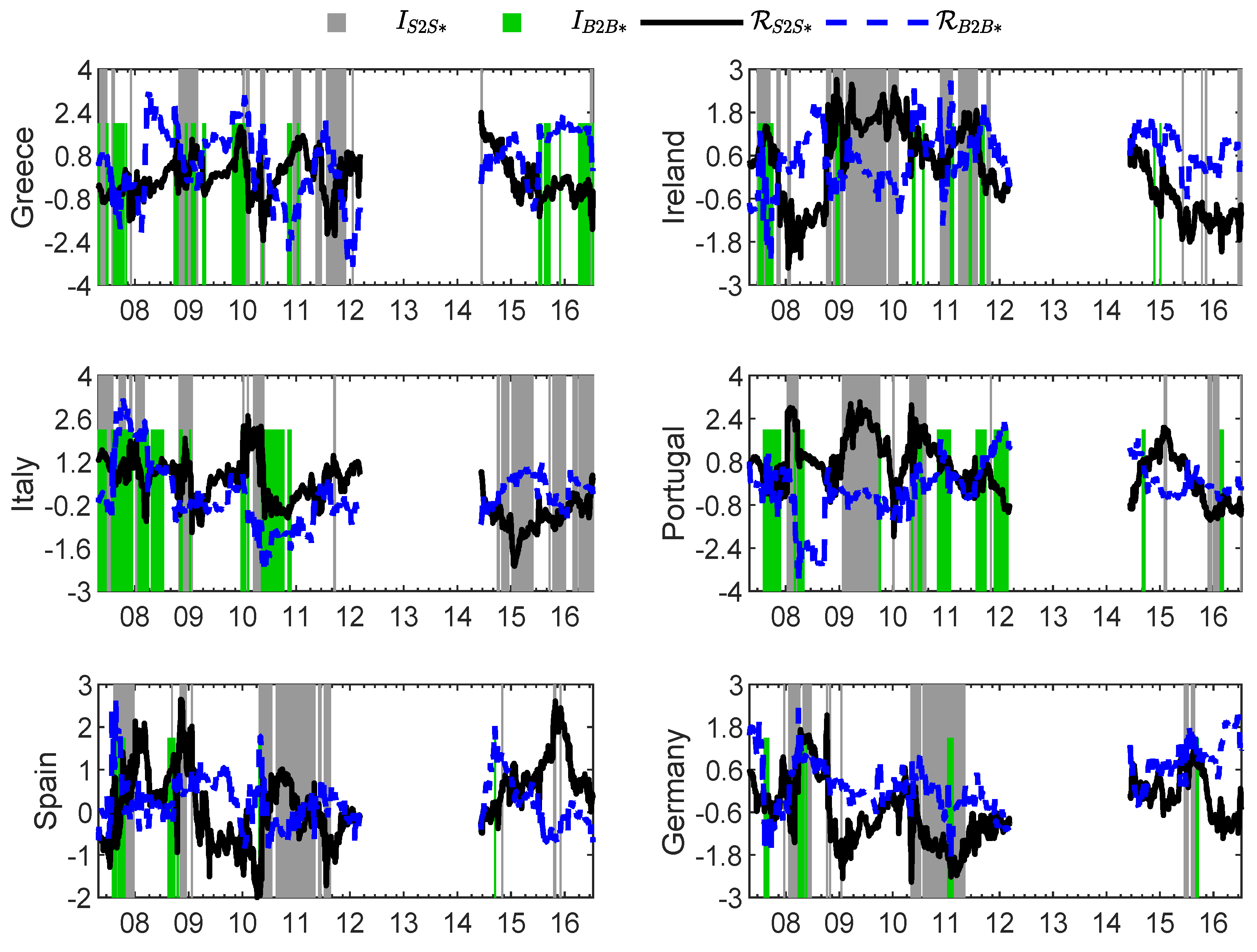
6. Within Sector Linkages

In Figure 3, significant episodes of Granger causality from banks in country i to all other banks (green shaded area) and from sovereigns in country i to all other sovereigns (gray shaded area), are superimposed over the average signed effect ${\overline{\mathcal{R}}}_{S2S\ast }\left(t\right)$ and ${\overline{\mathcal{R}}}_{B2B\ast }\left(t\right)$ for the GIIPS countries and Germany.

All of the countries show increased vulnerability in the banking sector at the beginning of the sample period in 2007, which then drops off significantly during 2008. The striking exception to this rule is Italy where, throughout 2008, the Italian banking system seems to maintain its ability to predict movements in CDS spreads in the banking sectors of the other GIIPS countries.

The channels of Granger causality then move to the sovereign sector in all of the GIIPS countries in 2009 when the sovereign sector experiences a sudden sharp increase in vulnerability just after the raft of bank bailouts in late 2008 following the collapse of Lehman Brothers. Not surprisingly, the evidence of information flow from the sovereign sector in Ireland and Portugal remains throughout 2009. These two countries both provided substantial government support their banking sectors. In mid-2010, there is another sharp increase in the flow of information in the sovereign sector, coinciding with increasing fear of excessive sovereign debt and the downgrading of the debt of Greece and Portugal by international credit agencies downgraded in April 2010. Ireland appears to behave slightly different with the increased evidence of connectivity occurring later than the other GIIPS countries. The appearance of the grey shaded area in Ireland coincides with the date when Moody’s downgraded Ireland’s credit rating by five places to BAA1 in December 2010.

The connectivity of the German sovereign sector has already been alluded to in the discussion of Table 2. In Figure 3, it is apparent that the signed effect of Granger causality from the German sovereign sector corresponding to the grey shaded area during 2010–2011 is negative. This result is consistent with sovereign CDS spreads in Germany being negatively correlated with the spreads in the other countries, suggesting that the Germany sovereign sector was stable and acting as a safe haven asset during this period, consistent with Dungey and Renault (2018) and Broto and Perez-Quiros (2015). This interpretation highlights the usefulness of the ability to sign the causal influences.

Another feature worth highlighting is that, just prior to the closure of the Greek sovereign market, there are significant causal effects flowing from Greece to the other sovereign sectors, but once again the sign of the influence is negative. A possible interpretation is that the widening default spreads in Greece to 10 times the levels being experienced elsewhere is responsible for the sign of the causal effects.

Finally, the influence of episodes of within sector Granger causality after the re-opening of the Greek sovereign market is fairly muted. This is true for both banking and sovereign sectors. In particular, there is no information flow in the Greek sovereign sector around the time of the vote by Greece not to adopt the austerity measures proposed by the European Union. After the re-opening of the Greek market, it is only the Italian sovereign sector which appears to provide information on the CDS spreads in the other GIIPS countries.

7. Linkages Between Sectors

The information flow between the two different sectors may be separated into two cases, namely, within country (the diagonal elements of the two off-diagonal blocks in Table 2) and across countries (the remaining elements in the off-diagonal blocks in Table 2).

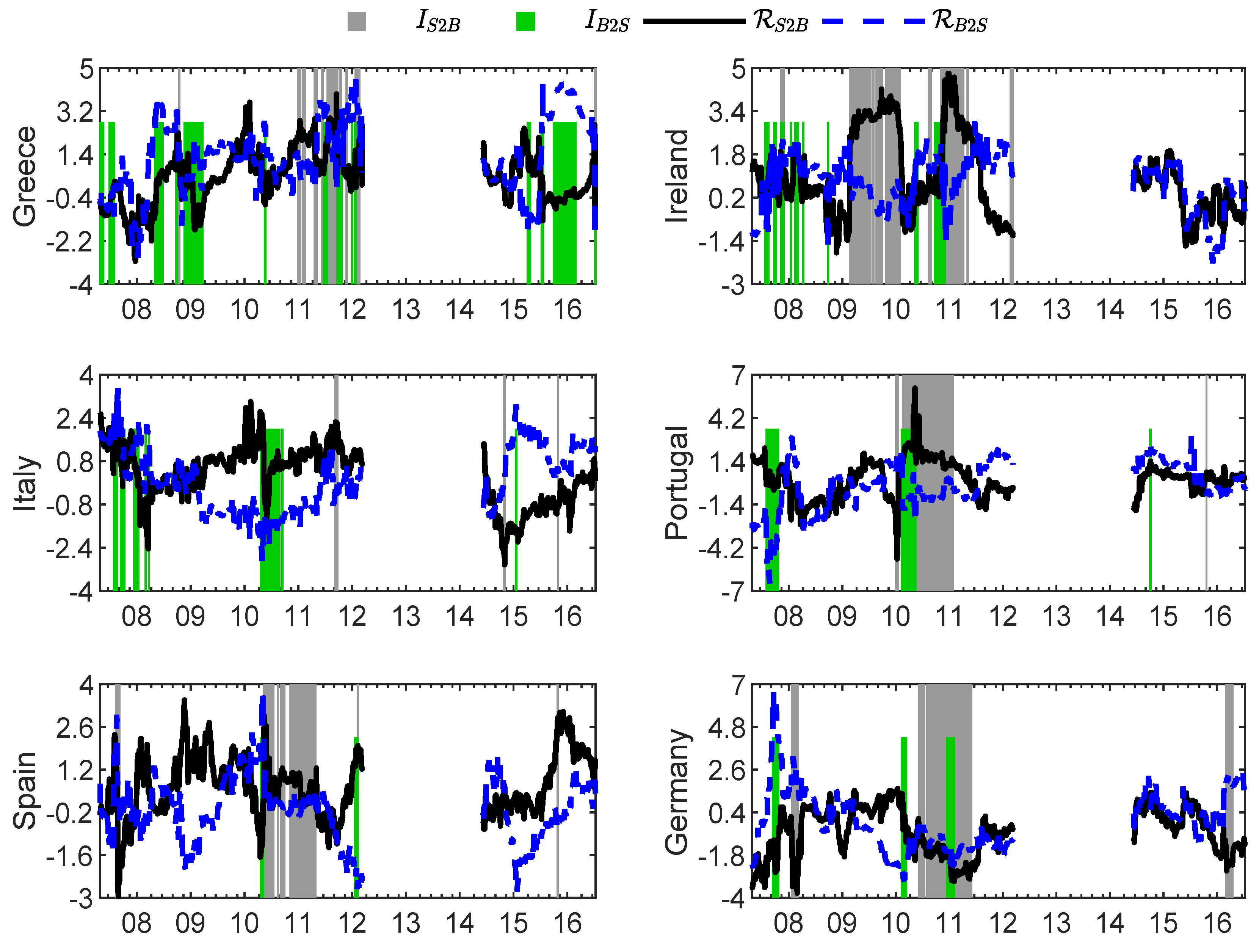
7.1. Within Countries

In this section, within country cross-sector risk transfers, as defined by the relationships in Equation (6), are examined. In Figure 4, significant episodes of Granger causality from sovereigns to banks in country i (green shaded area) and from banks to sovereign in country i (gray shaded area), are superimposed over the signed effects, ${\mathcal{R}}_{S2B}\left(t\right)$ and ${\mathcal{R}}_{B2S}\left(t\right)$, respectively, for the GIIPS countries and Germany.

Evidence of a feedback loop is provided by adjacent or overlapping gray and green shaded areas. Where this pattern occurs, a period of significant Granger causality from one sector to another is immediately followed by a period in which the direction of causality is reversed. This is precisely what is meant by a feedback, diabolical or doom loop as described in the Introduction. In this regard, Greece in the years 2011 and 2012 paints a devastating picture of a recurring diabolical loop that, based on the evidence in Figure 4, appears to originate in the sovereign sector. The Granger causal effects run first from sovereigns to banks and the loop continues until the evidence is shut down in March 2012. This instance provides support for the claim of Acharya et al. (2014) that the stress in the banking sector stems in part from the sovereign sector.

The most striking example of a domestic feedback loop is provided by Ireland in late 2010 and early 2011. In November 2010, Ireland agreed a package of financial aid from the European Union and IMF. There is a definite increase in the signed effect ${\mathcal{R}}_{B2S}\left(t\right)$ for Ireland, corresponding to the green shaded area where the Granger causal channel from banks to sovereigns opens. This is followed immediately by a large increase in the ${\mathcal{R}}_{S2B}\left(t\right)$ corresponding to the grey shaded area.

The preconditions for the Irish crisis relate to Ireland’s phenomenal growth during the prior decade, which featured rapid credit growth and over-extension by the banking sector in the housing market. In response to the banking crisis, the Irish government implemented a strong austerity program with the result that the source of the financial fragility moved to the sovereign sector. If any inference can be drawn about the origin of the financial crises, then the evidence here suggests that it is in the banking sector, thus providing support for the theory of Acemoglu et al. (2015) who hypothesize that the origins of financial fragility is in the banking sector.

Portugal and Spain also experience a domestic feedback loop in 2010–2011. In Portugal causality from banks to sovereigns appears first, as it also does (briefly) in Spain. Immediately after these episodes, there is an extended period of causality in the reverse in both these countries. The episode of vulnerability in the sovereign sector spreading to the banks in Spain corresponds to the period when Spain was mired in deep recession, with crippling unemployment among younger members of the population, aged between 15 and 25 years old.

The Italian banking sector appears to be an important source of information, a result which is consistent with the bold entries in Table 2. There is, however, no evidence of domestic feedback loops in Italy. Interestingly, Germany in 2010–2011 has a period of overlapping shading. Note, however, that the signed indices are negative indicative perhaps of a virtuous loop rather than the reverse.

Overall, the results support the existence of feedback loops in Greece, Ireland Portugal and Spain and all are consistently observed around the timeline of late 2010/early 2011. Only in the case of Greece are there multiple loops, and this evidence ends abruptly with the closing of the sovereign market. In three of the four cases, the first causal channel to open up is that from banks to sovereigns.

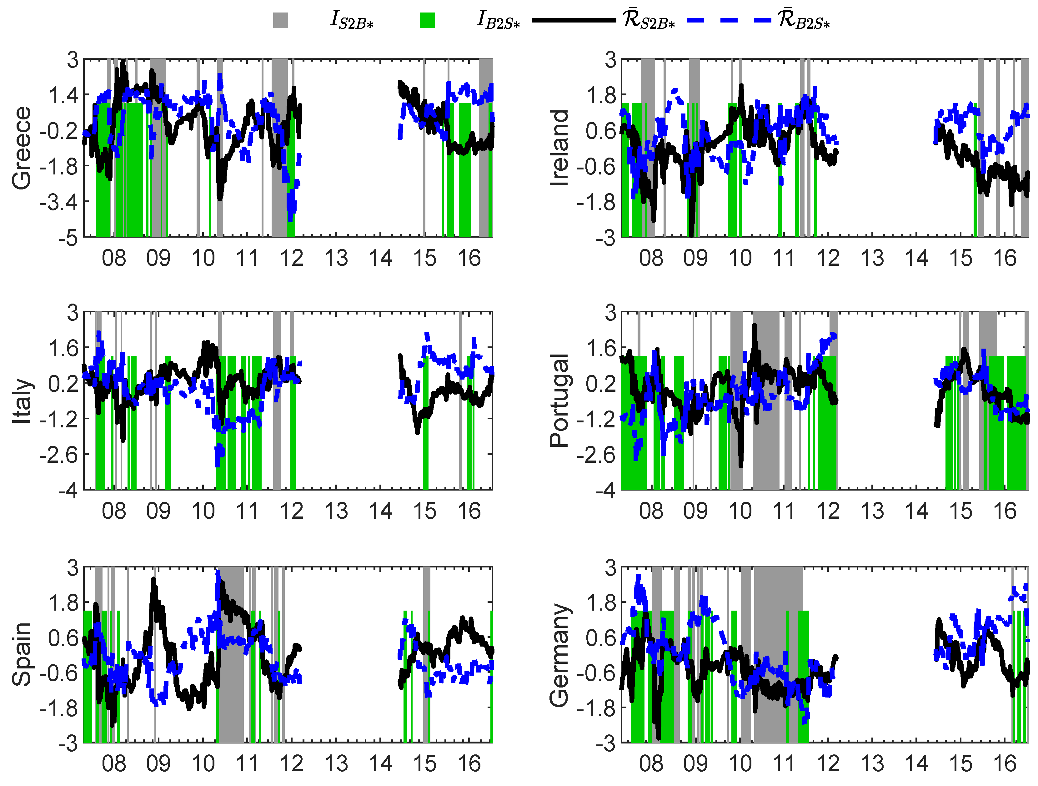
7.2. Across Countries

The relative importance of across country spillovers between sectors is illustrated in Figure 5. Significant episodes of Granger causality from sovereigns in country i to banks in all other countries (grey shaded area) and from banks in country i to sovereigns in all other countries (green shaded area), are superimposed over the average signed effect ${\overline{\mathcal{R}}}_{S2B\ast }\left(t\right)$ and ${\overline{\mathcal{R}}}_{B2S\ast }\left(t\right)$ for the GIIPS countries and Germany.

In general, the causal channel from banks to sovereigns in other countries dominates in the early part of the sample. In Italy and Portugal, this effect remains prominent right up to March 2012. In contrast, the causal effects from sovereigns to banks appears to be more concentrated in the time period from 2010 to 2012, starting in Portugal and Spain and then appearing in the Greek sovereign market in the lead up to the closure of the market. Once again, there is an extensive grey shaded area, indicating a causal channel from the German sovereign sector to the banking sectors of the GIIPS countries. As was the case, earlier, the sign of this effect is negative, indicative perhaps that falling CDS spreads in German sovereigns were predictive of rising CDS spreads in the banking sectors elsewhere.

Given the construction of the Granger causality tests in this section, no evidence of feedback loops can be deduced from these results. However, the general pattern found earlier is clearly reinforced, namely that the banking sector is responsible for information flow early in the sample during the sub-prime crises and the sovereign sector is the main source of information during the European debt crisis.

Turning to the period post 2014, information flow seems to be sporadic. The exception is connectivity between the Portuguese banks and the sovereign sectors of the other countries. As discussed in Section 5, this is likely to reflect concerns about the potential for government support for weak banks in other markets, akin to the wake-up call mechanism in the contagion literature.9

Given the extensive periods of causality indicated by the shaded areas in Figure 5, international connectivity between these two sectors is high. This prima facie evidence of an international dimension to the propagation of financial crises implies that cross-jurisdiction policy-making is likely to be extremely important in limiting the escalation of financial crises via feedback loops. Brunnermeier et al. (2016) argue that financial vulnerability and hence loops cannot be avoided by restricting banks’ sovereign exposures to remain within a country. They argue that to deal effectively with the propagation of crisis conditions, domestic regulators should diversify systemic risk across countries and sectors. This policy prescription seems to have some merit given the results reported here.

8. Conclusions

The paper demonstrates how econometric results generated by time-varying Granger causality tests, based on rolling windows and suitably adjusted for the issue of multiplicity, can shed light on the detection of potential feedback loops between sovereign debt and banking sectors during financial crises. The flexibility of the approach allows the relative importance of both domestic and cross country linkages between these sectors to be discovered and emphasizes that these linkages not only exist, but may reverse direction during crisis periods.

The results reported here indicate that global information transfer was highest during the sub-prime crises of 2007 and again in the European debt crisis of 2009–2010. A very consistent result is that the causal channel from banks to sovereigns (both domestic and international) is the first to open early on in the sample, followed later by the reverse channel from sovereigns to banks during the debt crisis. Evidence is found of domestic feedback loops in Greece, Ireland Portugal and Spain in late 2010/early 2011. Only in the case of Greece are there repeated loops; these are ultimately brought to an end by the closing of the Greek sovereign market in 2012. Three of the four instances of the domestic feedback loops appear to have their origin in the banking sector.

Our results also suggest very strongly that financial fragility is an international phenomenon. This may reflect the increasing internationalization and diversification of banking portfolios, and/or the general need for banks to hold high quality long-term debt to meet capital requirements. Both aspects point to the difficulty of a domestic regulator being able to deal with the propagation of crises across both borders and asset market instruments. These findings are important for policy makers. The solution to mitigating or preventing financial fragility and the potential development of feedback loops requires a framework which encompasses both possible directions and sources of transmission, as recently proposed in Fahri and Tirole (2018), although crucially, this must be extended to include the risk associated with both banking and sovereign debt cross-country jurisdictional considerations.