Asymptotic Theory for Cointegration Analysis When the Cointegration Rank Is Deficient

Abstract

We consider cointegration tests in the situation where the cointegration rank is deficient. This situation is of interest in finite sample analysis and in relation to recent work on identification robust cointegration inference. We derive asymptotic theory for tests for cointegration rank and for hypotheses on the cointegrating vectors. The limiting distributions are tabulated. An application to US treasury yields series is given.

1. Introduction

Determination of the cointegration rank is an important part of analyzing the cointegrated vector autoregressive model in the framework of Johansen (1988, 1991, 1995), Johansen and Juselius (1990), and Juselius (2006). We consider the rank deficient case where the cointegration rank of the data generating process is smaller than the rank used in the statistical analysis. In that case, the data generating process has more unit roots than the number of unit roots imposed in the statistical analysis and the usual asymptotic theory fails. We provide asymptotic theory for cointegration rank tests and tests on cointegration vectors along with simulated tables of the asymptotic distributions.

Cointegration analysis is conducted in three steps. First, the specification of the model is checked. Second, the rank is determined using a sequential procedure using Dickey-Fuller type distributions. Third, the cointegrating vectors are estimated and restrictions can be tested using standard inference. Asymptotic theory shows that estimated rank is consistent in the sense that the probability that the estimated rank is not equal to the true rank equals the size of tests, whereas the probability that the estimated rank is too small vanishes, see Johansen (1992, 1995) and Paruolo (2001). Hence, the rank deficiency problem does not arise in the asymptotic analysis.

In practice, rank deficiency matters in two ways. The asymptotic theory often suffers from considerable finite sample distortion. Further, if an investigator wants to focus on the inference on the cointegrating relations then problems can arise if the rank is taken as known when in fact it is deficient. These problems mirror those of instrumental variable estimation with weak instruments, see Mavroeidis et al. (2014).

When conducting inference on the cointegrating vector under near rank deficiency the parameters are weakly identified. At the extreme when testing on the cointegrating vector in the case of a deficient rank the model is mis-specified. This problem arises in cointegration as well as in instrumental variable estimation. In both cases maximum likelihood is conducted using reduced rank regression. The weak identification problem has attracted considerable attention in the instrumental variable literature, see for instance Mavroeidis et al. (2014). Khalaf and Urga (2014) discussed the weak identification problem for cointegration, that is when testing for a known cointegrating vector in the nearly rank deficient situation. These authors investigate various methods to adjust the asymptotic distribution in the weak identification case. This includes a bounds-based critical value suggested by Dufour (1997). This method requires knowledge of the asymptotic theory for the rank deficient case, which we provide here.

The practical problem of ignoring rank deficiency is illustrated using yield curve data. The expectation hypothesis is often interpreted as follows. Interest rates at different maturities are integrated series, but cointegrate so that spreads are stationary. Spreads are often found to be non-stationary. Thus, it is quite possible that a pair of interest rates do not cointegrate. An investigator may proceed by assuming cointegration when there is none, so that the rank is deficient, and conduct inference on the coefficients on the alleged cointegrating vector using standard inference. Our theory shows that the inference is then severely distorted. When the rank is deficient or nearly deficient it is incorrect to use standard inference on the cointegrating vectors. Nonetheless, applying standard inference in the particular example leads to marginal rejection of the hypothesis. Applying the bounds test of Khalaf and Urga (2014) shifts the distribution to the right and there is not much power to reject a hypothesis. If the rank is deficient, which is possible in the example, the alleged cointegrating vector cannot be cointegrating.

Rank deficiency also matters when the rank is determined empirically. Different asymptotic distributions arise in the standard case and when the rank is deficient. The asymptotic distribution tends to give a very good approximation to the finite sample distribution when the rank is far from being deficient, see for instance Nielsen (1997, 2004) When the parameters are in the vicinity of rank deficiency the finite sample distribution tends to be a combination of the two asymptotic distributions. When the parameters are not too close to the rank deficient case a Bartlett correction using a fixed parameter second-order asymptotic expansion works very well, see Johansen (2000, 2002) Bootstrap solutions have been discussed in simulation studies by Fachin (2000); Gredenhoff and Jacobson (2001); Swensen (2004); Cavaliere et al. (2012). When the parameters are closer to rank deficient a local-to-unity asymptotic expansion gives an improvement, see Nielsen (2004) for the cointegration case and Nielsen (1999, 2001) for the corresponding instrumental variable case. A starting point for the finite sample analysis is knowledge of the fixed-parameter first-order asymptotic theory across the parameter space, including rank deficient cases.

We discuss the asymptotic theory for models without and with deterministic terms in Section 2 and Section 3, respectively. The implications for finite sample analysis and the weakly identified case are discussed in Section 4 along with an application to US treasury zero coupon yields. Section 5 concludes. Proofs are given in an Appendix A.

2. The Model without Deterministic Terms

We consider the Gaussian cointegrated vector autoregressive model in the case with no deterministic terms. The asymptotic theory for tests for reduced cointegration rank and for a known cointegrating vector is derived when the rank is deficient. Finally, we analyze the case of near rank deficiency.

2.1. Model and Hypotheses

Consider a p-dimensional time series $X_t$ for $t=1-k,\cdots ,0,1,\cdots T$. The unrestricted vector autoregressive model can be written as

$$\Delta X_t=\Pi X_{t-1}+\sum _{i=1}^{k-1}{\mathsf{\Gamma }}_i\Delta X_{t-i}+{\epsilon }_t\mathrm{for}t=1,\cdots ,T,$$

(1)

where the innovations ${\epsilon }_t$ are independent normal ${\mathsf{N}}_p(0,\Omega )$-distributed. The parameters $\Pi$, ${\mathsf{\Gamma }}_i$, $\Omega$ are freely varying p-dimensional square matrices so that $\Omega$ is symmetric, positive definite.

The hypothesis of reduced cointegration rank is formulated as

$${\mathsf{H}}_z(r):\mathrm{rank}\Pi \le r,$$

(2)

for some $0\le r\le p$. The interpretation of the hypotheses follows from the Granger-Johansen representation presented in Section 2.2 below. The subscript z indicates that the model has a zero deterministic component. The rank hypotheses are nested so that

$${\mathsf{H}}_z(0)\subset \cdots \subset {\mathsf{H}}_z(r)\subset \cdots \subset {\mathsf{H}}_z(p).$$

(3)

The rank deficiency problem arises when testing the hypothesis ${\mathsf{H}}_z(r)$ when in fact the sub-hypothesis ${\mathsf{H}}_z(r-1)$ is satisfied. The rank is determined to be r if the hypothesis ${\mathsf{H}}_z(r)$ cannot be rejected while the sub-hypothesis ${\mathsf{H}}_z(r-1)$ is rejected. As a short-hand we write ${\mathsf{H}}_z^{\circ }(r)={\mathsf{H}}_z(r)\backslash {\mathsf{H}}_z(r-1)$ for this situation. The rank can be determined along the procedure outlined in Johansen (1992, 1995) [Section 12.1] and Paruolo (2001). In practice, these decisions are often marginal, hence the need to study the asymptotic theory of test statistics in the rank deficient case.

The rank hypothesis can equivalently be written as

$${\mathsf{H}}_z(r):\Pi =\alpha {\beta }^{\prime },$$

(4)

where $\alpha$ and $\beta$ are $p\times r$ matrices. The advantage of this formulation is that $\alpha$ and $\beta$ vary in vector spaces. The formulation does, however, allow rank deficiency where the rank of $\Pi$ is smaller than r. We follow Johansen (1991, Equation (2.2)) and refer to $\beta$ as the cointegrating vectors. We find the terminology useful, although it is ambiguous. Indeed, for a particular data generating process where $\Pi$ has rank less than r then the identity $\Pi =\alpha {\beta }^{\prime }$ can be satisfied while columns of $\beta$ may not be row-eigenvectors of $\Pi$ in which case ${\beta }^{\prime }{X}_t$ cannot be stationary. Even when $\Pi$ has rank r then ${\beta }^{\prime }{X}_t$ is only (approximately) stationary under the I(1) condition introduced below. However, from a statistical viewpoint, the estimator of $\Pi$ under the restriction of rank r will in a finite sample have rank r with probability one. In practice our only knowledge of the rank arises from inference. Johansen’s terminology appears to be focused on the statistical viewpoint which we will follow even when studying the rank deficient cases.

The hypothesis of known cointegration vectors is

$${\mathsf{H}}_{z,\beta }(r):\Pi =\alpha b^{\prime },$$

(5)

for some unknown matrix $\alpha$ and a known matrix b, both of dimension $p\times r$, so that b has full column rank. The standard analysis is concerned with the situation where $\alpha$ has full column rank, but in the rank deficient case, it has reduced column rank, so that the hypothesis ${\mathsf{H}}_z(r-1)$ is satisfied. When referring to b as the cointegrating vectors, we, once again, follow the terminology of Johansen (1991, Equation (3.1)) even though $b^{\prime }{X}_t$ cannot be stationary under rank deficiency.

2.2. Granger-Johansen Representation

The Granger-Johansen representation provides an interpretation of the cointegration model that is useful in the asymptotic analysis. We work with the result stated by Johansen (1995, Theorem 4.2). The theorem requires the following assumption.

I(1) Condition.

Suppose $\mathrm{rank}\Pi =s$ where $s\le p$. Consider the characteristic roots satisfying $0=det\{A(z)\}$ where $A(z)=(1-z)I_p-\Pi z-{\sum }_{i=1}^{k-1}{\mathsf{\Gamma }}_i{z}^i(1-z)$. Suppose there are $p-s$ unit roots, and that the remaining roots are stationary roots, so satisfying $\left|z\right|>1$.

The Granger-Johansen theorem assumes that a process satisfying the model (1) so that $\mathrm{rank}\Pi =r$ and we can write $\Pi =\alpha {\beta }^{\prime }$ while the I(1) condition holds with $s=r$. The process then has the representation

$$X_t=C\sum _{i=1}^t{\epsilon }_i+S_t+\tau ,$$

(6)

where the impact matrix C for the random walk has rank $p-r$ and satisfies ${\beta }^{\prime }C=0$ and $C\alpha =0$, the process $S_t$ can be given a zero mean stationary initial distribution and $\tau$ depends on the initial observations in such a way that ${\beta }^{\prime }\tau =0$. In other words, the process $X_t$ behaves like a random walk with cointegrating relations ${\beta }^{\prime }{X}_t$ that can be given a stationary initial distribution.

2.3. Test Statistics

The likelihood ratio test statistic for the reduced rank hypothesis ${\mathsf{H}}_z(r)$ against the unrestricted model ${\mathsf{H}}_z(p)$ is found by reduced rank regression, see Johansen (1995, Section 6). It can be described as a two-step procedure. First, the differences $\Delta X_t$ and the lagged levels $X_{t-1}$ are regressed on the lagged differences $\Delta X_{t-i}$, $i=1,\cdots ,k-1$ giving residuals $R_{0,t}$, $R_{1,t}$. Secondly, the squared sample correlations, $1\ge {\widehat{\lambda }}_1\ge \cdots \ge {\widehat{\lambda }}_p\ge 0$ say, of $R_{0,t}$ and $R_{1,t}$ are found, by computing product moments $S_{ij}=T^{-1}{\sum }_{t=1}^T{R}_{i,t}{R}_{j,t}^{\prime }$ and solving the eigenvalue problem $0=det(\lambda S_{11}-S_{10}{S}_{00}^{-1}{S}_{01})$. The log likelihood ratio test statistic for the rank hypothesis is then

$$LR\{{\mathsf{H}}_z(r)\mid {\mathsf{H}}_z(p)\}=-T\sum _{j=r+1}^{p}log(1-{\widehat{\lambda }}_j).$$

(7)

Under the hypothesis of known cointegration vectors, the likelihood is maximised by least squares regression. The log likelihood ratio test statistic against the unrestricted model ${\mathsf{H}}_z(p)$ is therefore given by

$$LR\{{\mathsf{H}}_{z,\beta }(r)\mid {\mathsf{H}}_z(p)\}=-Tlog\frac{det\{S_{00}-S_{01}{S}_{11}^{-1}{S}_{10}\}}{det\{S_{00}-S_{01}b{(b^{\prime }{S}_{11}b)}^{-1}{b}^{\prime }{S}_{10}\}}.$$

(8)

The log likelihood ratio statistic for the hypothesis of known cointegrating vector against the rank hypothesis is found by combining the statistics in (7) and (8), that is

$$LR\{{\mathsf{H}}_{z,\beta }(r)\mid {\mathsf{H}}_z(r)\}=LR\{{\mathsf{H}}_{z,\beta }(r)\mid {\mathsf{H}}_z(p)\}-LR\{{\mathsf{H}}_z(r)\mid {\mathsf{H}}_z(p)\}.$$

(9)

The relationship will be useful in the asymptotic theory. For instance, Theorems 1 and 2 give the asymptotic distributions of $LR\{{\mathsf{H}}_z(r)\mid {\mathsf{H}}_z(p)\}$ and $LR\{{\mathsf{H}}_{z,\beta }(r)\mid {\mathsf{H}}_z(p)\}$, respectively. From this we can derive an expression for the distribution of $LR\{{\mathsf{H}}_{z,\beta }(r)\mid {\mathsf{H}}_z(r)\}$. When it comes to tabulation we will need to simulate all three distributions. This would be the case even if the former two statistics were independent.

2.4. Asymptotic Theory for the Rank Test

In the asymptotic analysis it is possible to relax the assumption to the innovations. While the likelihood is derived under the assumption of independent, identically Gaussian distributed innovations less is needed for the asymptotic theory. Johansen (1995) assumes the innovations are independent, identically distributed with mean zero and finite variance and uses linear process results from Phillips and Solo (1992). This could be relaxed further to, for instance, a martingale difference assumption. However, for expositional simplicity we follow Johansen’s argument and assumptions.

Theorem 1.

Consider the rank hypothesis ${\mathsf{H}}_z(r):\mathrm{rank}\Pi \le r$. Suppose ${\mathsf{H}}_z^{\circ }(s)={\mathsf{H}}_z(s)\backslash {\mathsf{H}}_z(s-1)$ holds for some $s\le r$ and that the I(1) condition holds for that s. Let $F_u=B_u$ be a $p-s$-dimensional standard Brownian motion on $[0,1]$. Let $1\ge {\rho }_1\ge \cdots \ge {\rho }_{p-s}\ge 0$ be the eigenvalues of the eigenvalue problem

$$0=det\left\{\rho {\int }_0^1{F}_u{F}_u^{\prime }du-{\int }_0^1{F}_u{(d{B}_u)}^{\prime }{\int }_0^1(d{B}_u)F_u^{\prime }\right\}$$

(10)

Then, for $T\to \infty$,

$$LR\{{\mathsf{H}}_z(r)\mid {\mathsf{H}}_z(p)\}=-T\sum _{j=r+1}^{p}log(1-{\widehat{\lambda }}_j)\stackrel{\mathsf{D}}{\to }\sum _{j=r-s+1}^{p-s}{\rho }_j.$$

(11)

In the standard non-deficient situation where $r=s$ the result reduces to the result of Johansen (1995, Theorem 6.1). The rank deficient case was also discussed by Johansen (1995, p. 158) and Nielsen (2004, Theorem 6.1).

Table 1 reports the asymptotic distribution of the rank test reported in Theorem 1. The simulation were done using Ox (Doornik 2007). The simulation design follows that of Johansen (1995, Section 15). That is, the stochastic integrals in (10) were descretized with $T=1000$ and zero initial observations with one million repetitions. The table reports simulated quantiles and moments for $r-s=0,1,2$ and $p-r=1,2,3,4$. However, the case of $p-r=1$ and $r-s=0$ are analytic values from Nielsen (1997) and where the quantiles were provided by Karim Abadir using his results in Abadir (1995). Bernstein (2014) reports values for higher dimensions. The 85% quantile has not been computed analytically in this case.

Table 1. Quantiles, mean, and variance of $LR\{{\mathsf{H}}_z(r)|{\mathsf{H}}_z(p)\}$, where the data generating process has rank $s=\mathrm{rank}\Pi \le r$.

$\mathit{r}-\mathit{s}$	$\mathit{p}-\mathit{r}$	50%	80%	85%	90%	95%	97.5%	99%	Mean	Var
0	1	0.60	1.88	—	2.98	4.13	5.32	6.94	1.14	2.22
	2	5.48	8.48	9.31	10.44	12.30	14.07	16.34	6.09	10.61
	3	14.39	18.94	20.13	21.70	24.22	26.54	29.37	15.02	25.13
	4	27.29	33.35	34.88	36.91	40.04	42.93	46.45	27.93	45.66
1	1	0.36	1.13	1.38	1.74	2.35	2.98	3.81	0.67	0.70
	2	4.27	6.25	6.78	7.50	8.65	9.76	11.14	4.61	4.66
	3	11.92	15.20	16.04	17.14	18.88	20.50	22.48	12.31	13.22
	4	23.47	28.09	29.25	30.76	33.10	35.21	37.83	23.89	26.96
2	1	0.30	0.97	1.18	1.48	1.98	2.47	3.11	0.56	0.48
	2	3.93	5.57	6.01	6.59	7.51	8.38	9.46	4.18	3.24
	3	11.04	13.82	14.53	15.46	16.91	18.24	19.87	11.34	9.63
	4	21.84	25.83	26.82	28.11	30.09	31.91	34.13	22.18	20.21

The first panel of Table 1 reports the distribution for the standard case where $s=r$. This corresponds to Table 15.1 of Johansen (1995). The second and third panel of Table 1 report the distribution for the rank deficient case where $s=r-1$ so $r-s=1$ and where $s=r-2$ so $r-s=2$. The first entry in panel 2 for $s=r-1$ and $p-r=1$, so $r-s=1$, corresponds to Table 6 of Nielsen (2004). It is seen that as the rank becomes more deficient the distribution shifts to the left. It should be noted that if the rank is non deficient, but the I(1) condition is not satisfied then the distribution would tend to shift to the right, see Nielsen (2004) for a discussion. The simulations reported in Table 8 of that paper indicates that the distribution is between these extremes if the rank is deficient and the I(1) condition fails.

The rank test statistic in (7) has been analyzed analytically for the canonical correlation problem in cross-sectional models in Nielsen (1999, 2001) This test also corresponds to the test for relevance in the instrument variable problem. In that case, analytic expressions are available when $p=2$, $r=1$ and $s=0,1$. When $s=1$ we have a ${\chi }^2$-distribution with mean 1 and variance 2. When $s=0$ the mean is 0.429 and the variance is $0.575-{(0.429)}^2=0.391$, see Nielsen (1999). Thus, the impact of rank deficiency is similar to what is seen in Table 1 for cointegration rank testing.

2.5. Asymptotic Theory for the Test on the Cointegrating Vectors

In the analysis of the test for known cointegrating vectors, we focus on the situation where the data generating process has rank $s=0$. In this situation the asymptotic distribution is relatively simple to describe, because it does not depend on the value of the hypothesized cointegrating vectors b. This is adequate for a discussion of aspects of situations considered in Khalaf and Urga (2014). If the rank is non-zero but deficient so $0<s<r$, then the data generating process will have cointegrating vectors ${\beta }_0$ of dimension $p\times s$ and the asymptotic theory will depend on ${\beta }_0$ and b. In practice, it is rare to test for simple hypotheses when there is more than one hypothesized cointegrating vector, so we do not pursue this complication.

The analysis of the test for known cointegrating vectors is somewhat different from the analysis in Johansen (1995). His analysis is aimed at the situation where different restrictions are imposed on the cointegrating vectors. The argument then involves an intriguing consistency proof for the estimated cointegrating vectors. However, when testing the hypothesis of known cointegrating vectors the likelihood is maximized by the least squares method and the consistency argument is not needed. The asymptotic theory can then be described by the following result.

Theorem 2.

Consider the hypothesis ${\mathsf{H}}_{z,\beta }(r):\Pi =\alpha b^{\prime }$, where $\alpha ,b$ have dimension $p\times r$ and where α is unknown and b is known with full column rank. Suppose ${\mathsf{H}}_z(0)$ is satisfied, so that $\alpha =0$ and $s=0$, and that the I(1) condition is satisfied with $s=0$. Let $B_u$ be a p-dimensional standard Brownian motion on $[0,1]$ with components $B_{1,u}$ and $B_{2,u}$ of dimension r and $p-r$, respectively. Then, for $T\to \infty$,

$$\begin{array}{c}LR\{{\mathsf{H}}_{z,\beta }(r)\mid {\mathsf{H}}_z(p)\}\stackrel{\mathsf{D}}{\to }\mathrm{tr}\{{\int }_0^{1}d{B}_u{B}_u^{\prime }{({\int }_0^1{B}_u{B}_u^{\prime }du)}^{-1}{\int }_0^1{B}_u{(d{B}_u)}^{\prime }\hfill \\ -{\int }_0^{1}d{B}_u{B}_{1,u}^{\prime }{({\int }_0^1{B}_{1,u}{B}_{1,u}^{\prime }du)}^{-1}{\int }_0^1{B}_{1,u}{(d{B}_u)}^{\prime }\}.\hfill \end{array}$$

(12)

The convergence of the test statistic $LR\{{\mathsf{H}}_{z,\beta }(r)\mid {\mathsf{H}}_z(p)\}$ holds jointly with the convergence for the rank test statistic $LR\{{\mathsf{H}}_z(r)\mid {\mathsf{H}}_z(p)\}$, for $s=0$, in Theorem 1. Thus, when $s=0$ the formula (9) implies that the limit distribution of the test statistic for known β within the model with rank of at most r can be found as the difference of the two limiting variables.

Table 2 reports the asymptotic distribution of the test for known cointegrating vector in the model where the rank is at most r. When $s=r$ the asymptotic distribution is ${\chi }^2$ with $r(p-r)$ degrees of freedom, see Johansen (1995, Theorem 7.2.1). When $s=0$ the asymptotic distribution reported in Theorem 2 applies. The simulation design is as before. It is seen that in the rank deficient case the distribution is shifted to the right. This matches the finite sample simulations reported by Johansen (2000, Table 2).

Table 2. Quantiles, mean, and variance of $LR\{{\mathsf{H}}_{z,\beta }(r)|{\mathsf{H}}_z(r)\}$, where the data generating process has rank $s=\mathrm{rank}\Pi \le r$.

p	r	s	50%	80%	85%	90%	95%	97.5%	99%	Mean	Var
2	1	1	0.45	1.64	2.07	2.71	3.84	5.02	6.63	1	2
		0	2.62	5.44	6.22	7.30	9.05	10.75	12.96	3.31	8.71
3	2	2	1.39	3.22	3.79	4.61	5.99	7.38	9.21	2	4
		0	5.80	9.42	10.40	11.71	13.82	15.77	18.27	6.42	15.53
3	1	1	1.39	3.22	3.79	4.61	5.99	7.38	9.21	2	4
		0	6.79	10.58	11.57	12.89	15.02	17.00	19.49	7.33	17.52

Table 3 reports the simulated asymptotic distribution of the test for known cointegrating vector in the model where the rank is unrestricted. The distribution is shifted to the right in the rank deficient case. Note, that the table reports the distribution of the convolution of the statistics simulated in Table 1 and Table 2, see (9). Thus, up to a simulation error the expectations reported in Table 1 and Table 2 add up to the expectation reported in Table 3. In the full rank case $r=s$ the statistics in Table 1 and Table 2 are independent, as proved below, so also the variances are additive.

Table 3. Quantiles, mean, and variance of $LR\{{\mathsf{H}}_{z,\beta }(r)|{\mathsf{H}}_z(p)\}$, where the data generating process has rank $s=\mathrm{rank}\Pi \le r$.

p	r	s	50%	80%	85%	90%	95%	97.5%	99%	Mean	Var
2	1	1	1.54	3.43	4.01	4.83	6.22	7.62	9.47	2.15	4.23
		0	3.35	6.11	6.89	7.95	9.70	11.38	13.57	3.98	8.82
3	2	2	2.52	4.85	5.53	6.48	8.07	9.60	11.62	3.15	6.26
		0	6.36	9.96	10.92	12.22	14.32	16.29	18.79	6.98	15.35
3	1	1	7.50	11.03	11.98	13.27	15.34	17.30	19.81	8.13	14.73
		0	11.33	15.73	16.88	18.41	20.83	23.09	25.91	11.96	23.31

Theorem 3.

Consider the hypothesis ${\mathsf{H}}_{z,\beta }^{\circ }(r)$. Suppose ${\mathsf{H}}_z^{\circ }(r)={\mathsf{H}}_z^{\circ }(r)/{\mathsf{H}}_z^{\circ }(r-1)$ is satisfied and that the $I(1)$ condition holds with $s=r$. Then the rank test statistic $LR\{{\mathsf{H}}_z^{\circ }(r)|{\mathsf{H}}_z^{\circ }(p)\}$ and the statistic $LR\{{\mathsf{H}}_{z,\beta }^{\circ }(r)|{\mathsf{H}}_z^{\circ }(r)\}$ for testing a simple hypothesis on the cointegrating vector are asymptotically independent.

The asymptotic distribution of the rank statistic $LR\{{\mathsf{H}}_z^{\circ }(r)|{\mathsf{H}}_z^{\circ }(p)\}$ is given in Theorem 1, while the statistic for the cointegrating vector $LR\{{\mathsf{H}}_{z,\beta }^{\circ }(r)|{\mathsf{H}}_z^{\circ }(r)\}$ is asymptotically ${\chi }^2\{r(p-r)\}$.

2.6. The Case of Nearly Deficient Rank

With the above results we have two extremes. First, the full rank case where standard results apply, that is Johansen’s Dickey-Fuller type distribution for rank testing and ${\chi }^2$ inferences for testing constraints on the cointegrating vectors. Second, the rank deficient case where new Dickey-Fuller type distributions apply both for rank testing and for testing constraints on the cointegrating vectors. In between these extremes we have the nearly rank deficient case corresponding to weak identification in the instrumental variable literature. These nearly deficient cases can be analyzed using local-to-unity parametrization. However, a full theory is notationally complicated as there will be many nuisance parameters. We therefore consider a simple special case inspired by the power analysis of Johansen (1995, Section 14) and distribution analysis of Nielsen (2004).

The main finding is that the appropriate local rate is $T^{-1}$ as in power analysis for unit tests and cointegration rank tests as opposed to $T^{-1/2}$ for stationary models as in Andrews and Cheng (2012). Consider a bivariate, first order, local-to-unity vector autoregressive model where

$$\Delta X_t=\frac{1}{T}\left(\begin{array}{cc}{b}_1& b_2\\ 0& 0\end{array}\right)X_{t-1}+{\epsilon }_t\mathrm{for}t=1,\cdots ,T,$$

(13)

where the innovations ${\epsilon }_t$ are independent normal ${\mathsf{N}}_2(0,I_2)$-distributed where $b_1\ne 0$.

We now have the following variant of the result for the rank test in Theorem 1.

Theorem 4

(Nielsen 2004, Theorem 6.2). Consider the data generating process (13). Let $B_u$ be a bivariate standard Brownian motion on $[0,1]$ and let $J_u$ be the bivariate Ornstein-Uhlenbeck process given by

$$J_u=\left(\begin{array}{cc}{b}_1& b_2\\ 0& 0\end{array}\right){\int }_0^u{J}_{s}ds+B_u.$$

Let $1\le {\rho }_1\le {\rho }_2\le 0$ be the eigenvalues of the eigenvalue problem

$$0=det\left\{\rho {\int }_0^1{J}_u{J}_u^{\prime }du-{\int }_0^1{J}_u{(d{B}_u)}^{\prime }{\int }_0^1(d{B}_u)J_u^{\prime }\right\}$$

Then, for $T\to \infty$,

$$LR\{{\mathsf{H}}_z(1)\mid {\mathsf{H}}_z(2)\}\stackrel{\mathsf{D}}{\to }{\rho }_2.$$

The limit distribution is tabulated in Nielsen (2004, Table 8).

We now consider the test for known cointegrating vector, $b={(b_1,b_2)}^{\prime }$. The result in Theorem 2 is modified as follows.

Theorem 5.

Consider the data generating process (13). Let $B_u,J_u$ be defined as in Theorem 4 and let $J_{1,u}=b^{\prime }{J}_u$. Then

$$\begin{array}{c}LR\{{\mathsf{H}}_{z,\beta }(1)\mid {\mathsf{H}}_z(2)\}\stackrel{\mathsf{D}}{\to }\mathrm{tr}\{{\int }_0^{1}d{B}_u{J}_u^{\prime }{({\int }_0^1{J}_u{J}_u^{\prime }du)}^{-1}{\int }_0^1{J}_u{(d{B}_u)}^{\prime }\hfill \\ {\int }_0^{1}d{B}_u{J}_{1,u}^{\prime }{({\int }_0^1{J}_{1,u}{J}_{1,u}^{\prime }du)}^{-1}{\int }_0^1{J}_{1,u}{(d{B}_u)}^{\prime }\}.\hfill \end{array}$$

3. The Model with a Constant

We now consider the model augmented with a constant. In the cointegrated model the constant is restricted to the cointegrating space. Thus, the cointegrating vectors consist of vectors relating the dynamic variable extended by a further coordinate for the constant. There are now two rank conditions; one related to the dynamic part of these extended cointegrating vectors and one relating to the deterministic part of the cointegrating vectors. The condition to the cointegration rank in the standard theory can therefore fail in two ways.

3.1. Model and Hypotheses

The unrestricted vector autoregressive model is

$$\Delta X_t=\Pi X_{t-1}+\mu +\sum _{i=1}^{k-1}{\mathsf{\Gamma }}_i\Delta X_{t-i}+{\epsilon }_t\mathrm{for}t=1,\cdots ,T,$$

(14)

where the innovations ${\epsilon }_t$ are independent normal ${\mathsf{N}}_p(0,\Omega )$-distributed. The parameters are the p-dimensional square matrices $\Pi$, ${\mathsf{\Gamma }}_i$, $\Omega$ and the p-vector $\mu$. They vary freely so that $\Omega$ is symmetric, positive definite.

For the model with a constant there are two types of cointegration rank hypotheses:

$$\begin{array}{cccc}\hfill {\mathsf{H}}_{c\ell }(r):& \hfill & \hfill \mathrm{rank}\Pi & \le r,\hfill \end{array}$$

(15)

$$\begin{array}{cccc}\hfill {\mathsf{H}}_c(r):& \hfill & \hfill \mathrm{rank}(\Pi ,\mu )& \le r.\hfill \end{array}$$

(16)

Their interpretations follow from the Granger-Johansen representation which is reviewed in Section 3.2 below. In short, if there are no rank deficiencies the first hypothesis ${\mathsf{H}}_{c\ell }$ gives cointegrating relations with a constant level and common trends with a linear trend. The second hypothesis ${\mathsf{H}}_c$ has a constant level both for the cointegrating relations and the common trends. The hypotheses are nested so that

$${\mathsf{H}}_c(0)\subset {\mathsf{H}}_{c\ell }(0)\subset \cdots \subset {\mathsf{H}}_{c\ell }(r-1)\subset {\mathsf{H}}_c(r)\subset {\mathsf{H}}_{c\ell }(r)\subset \cdots \subset {\mathsf{H}}_c(p)={\mathsf{H}}_{c\ell }(p).$$

(17)

This nesting structure is considerably more complicated than the structure (3) for the model without deterministic terms. A practical investigation may start in three different ways. First, the model (14) is taken as the starting point. Both types of hypotheses come into play and the rank is determined as outlined in Johansen (1995, Section 12). Secondly, if visual inspection of the data indicates that linear trends are not present the hypotheses ${\mathsf{H}}_{c\ell }$ may be ignored. Thirdly, if visual inspection of the data indicates that a linear trend could be present, the model (14) should be augmented with a linear trend term and we move outside the present framework. Nielsen and Rahbek (2000) discuss the latter two possibilities. Here, we are concerned with the first two possibilities.

The rank hypotheses can equivalently be formulated as

$$\begin{array}{cccc}\hfill {\mathsf{H}}_{c\ell }(r):& \hfill & \hfill \Pi & =\alpha {\beta }^{\prime },\hfill \end{array}$$

(18)

$$\begin{array}{cccc}\hfill {\mathsf{H}}_c(r):& \hfill & \hfill (\Pi ,\mu )& =\alpha ({\beta }^{\prime },{\beta }_c^{\prime }).\hfill \end{array}$$

(19)

The hypotheses of known cointegrating vectors are therefore

$$\begin{array}{cccc}\hfill {\mathsf{H}}_{c\ell ,\beta }(r):& \hfill & \hfill \Pi & =\alpha b^{\prime },\hfill \end{array}$$

(20)

$$\begin{array}{cccc}\hfill {\mathsf{H}}_{c,\beta }(r):& \hfill & \hfill (\Pi ,\mu )& =\alpha (b^{\prime },b_c^{\prime }).\hfill \end{array}$$

(21)

for a known $(p\times r)$-matrix b with full column rank and, in the second case, also a known $(1\times r)$-matrix $b_c$ so that $b^{*}={(b^{\prime },b_c^{\prime })}^{\prime }$ has full column rank.

3.2. Granger-Johansen Representation

We give a Granger-Johansen representation for each of the two reduced rank hypotheses. Both results follow from Theorem 4.2 and Exercise 4.5 of Johansen (1995). First, consider the hypothesis ${\mathsf{H}}_{c\ell }(r)$. Suppose that the sub-hypothesis ${\mathsf{H}}_c(r)$ does not hold and that the I(1) condition holds with $s=r$. Thus, the $(p\times r)$-matrices $\alpha ,\beta$ have full column rank but ${\alpha }_{\perp }^{\prime }\mu \ne 0$, so that the matrix ${\Pi }^{*}=(\Pi ,\mu )$ has rank $r+1$. Then, the Granger-Johansen representation is

$$X_t=C\sum _{i=1}^t{\epsilon }_i+S_t+{\tau }_c+{\tau }_{\ell }t,$$

(22)

where the impact matrix C has rank $p-r$ and satisfies ${\beta }^{\prime }C=0$ and $C\alpha =0$ while ${\tau }_{\ell }=C\mu \ne 0$. As a consequence, the process has a linear trend, but the cointegrating relations ${\beta }^{\prime }{X}_t$ do not have a linear trend, since ${\beta }^{\prime }C=0$.

Secondly, consider the hypothesis ${\mathsf{H}}_c(r)$. Suppose that the sub-hypothesis ${\mathsf{H}}_{c\ell }(r-1)$ does not hold and that the I(1) condition holds with $s=r$. Thus, the $(p\times r)$-matrices $\alpha ,\beta$ have full column rank, and the $\{(p+1)\times r\}$-matrix ${\beta }^{*}={(\beta ,{\beta }_c^{\prime })}^{\prime }$ has full column rank. Then, the Granger-Johansen representation (22) holds with ${\tau }_{\ell }=0$, while ${\tau }_c$ has the property that ${\beta }^{\prime }{\tau }_c=-{\beta }_c^{\prime }$. In other words, the process $X_t$ behaves like a random walk where ${\beta }^{\prime }{X}_t$ has an invariant distribution with a non-zero mean, while ${\beta }^{\prime }{X}_t+{\beta }_c^{\prime }$ has a zero mean invariant distribution.

3.3. Test Statistics

The test statistics are variations of those for the model without deterministic terms. The differences relate to the formation of the residuals $R_{0,t}$ and $R_{1,t}$.

First, consider the reduced rank hypothesis ${\mathsf{H}}_{c\ell }(r)$ and the corresponding hypothesis ${\mathsf{H}}_{c\ell ,\beta }(r)$ of known cointegrating vectors. The residuals $R_{0,t}$ and $R_{1,t}$ are formed by regressing the differences $\Delta X_t$ and the lagged levels $X_{t-1}$ on an intercept and the lagged differences $\Delta X_{t-i}$, $i=1,\cdots ,k-1$. In the second step, compute the canonical correlations $1\ge {\widehat{\lambda }}_1\ge \cdots \ge {\widehat{\lambda }}_p\ge 0$ of $R_{0,t}$ and $R_{1,t}$. The rank test statistic $LR\{{\mathsf{H}}_{c\ell }(r)|{\mathsf{H}}_{c\ell }(p)\}$ then has the form (7). The test statistic for known cointegrating vectors $LR\{{\mathsf{H}}_{c\ell ,\beta }(r)|{\mathsf{H}}_{c\ell }(p)\}$ has the form (8), using the same residuals $R_{0,t}$ and $R_{1,t}$, and the hypothesized cointegrating vectors b.

Secondly, consider the reduced rank hypothesis ${\mathsf{H}}_c(r)$ and the corresponding hypothesis ${\mathsf{H}}_{c,\beta }(r)$ of known cointegrating vectors. The residuals $R_{0,t}$ and $R_{1,t}$ are formed by regressing the differences $\Delta X_t$ and the vector formed by stacking the lagged levels and an intercept $X_{t-1}^{*}={(X_{t-1}^{\prime },1)}^{\prime }$ on the lagged differences $\Delta X_{t-i}$, $i=1,\cdots ,k-1$. In the second step, compute the canonical correlation of these $R_{0,t}$ and $R_{1,t}$. The rank test statistic $LR\{{\mathsf{H}}_c(r)|{\mathsf{H}}_c(p)\}$ then has the form (7). The test statistic for known cointegrating vectors $LR\{{\mathsf{H}}_{c,\beta }(r)|{\mathsf{H}}_c(p)\}$ has the form (8), using the same residuals $R_{0,t}$ and $R_{1,t}$, and the hypothesized cointegrating vectors $b^{*}={(b^{\prime },b_c^{\prime })}^{\prime }$.

3.4. Asymptotic Theory for the Rank Tests

There are now four situations to consider. Indeed, the nesting structure in (17) shows that each of the two rank hypotheses ${\mathsf{H}}_{c\ell }(r)$ and ${\mathsf{H}}_c(r)$ can be rank deficient in two ways when either of ${\mathsf{H}}_{c\ell }^{\circ }(s)={\mathsf{H}}_{c\ell }(s)/{\mathsf{H}}_c(s)$ or ${\mathsf{H}}_c^{\circ }(s)={\mathsf{H}}_c(s)/{\mathsf{H}}_{c\ell }(s-1)$ holds. In three cases the limiting distribution is of the same form as in Theorem 1, albeit with a different limiting random function $F_u$. In the fourth case the limiting distribution has nuisance parameters. The nuisance parameter case arises when testing ${\mathsf{H}}_c(r)$ with a data generating process satisfying ${\mathsf{H}}_{c\ell }^{\circ }(s)={\mathsf{H}}_{c\ell }(s)/{\mathsf{H}}_c(s)$. This is the case that can often be ruled out through visual inspection of the data as mentioned in Section 3.1.

We start with the test for the hypothesis ${\mathsf{H}}_{c\ell }(r)$ in the rank deficient case where ${\mathsf{H}}_{c\ell }^{\circ }(s)={\mathsf{H}}_{c\ell }(s)/{\mathsf{H}}_c(s)$ holds for $s<r$. Johansen (1995) discusses the possibility ${\mathsf{H}}_c^{\circ }(r)$. The asymptotic theory is as follows.

Theorem 6.

Consider the rank hypothesis ${\mathsf{H}}_{c\ell }(r):\mathrm{rank}\Pi \le r$. Suppose ${\mathsf{H}}_{c\ell }^{\circ }(s)={\mathsf{H}}_{c\ell }(s)\backslash {\mathsf{H}}_c(s)$ holds for some $s\le r$, so that $\mathrm{rank}\Pi =s$ and $\mathrm{rank}(\Pi ,\mu )=s+1$ and that the I(1) condition is satisfied for that s. Let $B_u$ be a $(p-s)$-dimensional standard Brownian motion on $[0,1]$. Define a $(p-s)$-dimensional vector $F_u$ with coordinates

$$F_{i,u}=\left\{\begin{array}{cc}{B}_{i,u}-{\overline{B}}_i\hfill & fori=1,\cdots ,p-s-1\hfill \\ u-1/2\hfill & fori=p-s\hfill \end{array}\right.$$

Then $LR\{{\mathsf{H}}_{c\ell }(r)\mid {\mathsf{H}}_{c\ell }(p)\}$ converges as in (11) using the present F.

Table 4 reports the simulated asymptotic distribution of the rank test reported in Theorem 6. The first panel gives the standard case where $s=r$ and corresponds to Johansen (1995, Table 15.3). For $p-r=1$ the asymptotic distribution is actually ${\chi }^2$ and the numbers are the standard numerically calculated ones rather than simulated ones. The second and the third panel report the distribution for the rank deficient case ${\mathsf{H}}_{c\ell }^{\circ }(s)$ where ${\mathsf{H}}_{c\ell }(s)$ holds, but ${\mathsf{H}}_c(s)$ fails. The distribution is shifted to the left when $r-s>0$ as in Table 1.

Table 4. Quantiles, mean, and variance of $LR\{{\mathsf{H}}_{c\ell }(r)|{\mathsf{H}}_{c\ell }(p)\}$, where the data generating process satisfies ${\mathsf{H}}_{c\ell }^{\circ }(s)={\mathsf{H}}_{c\ell }(s)\backslash {\mathsf{H}}_c(s)$ with $s\le r$.

$\mathit{r}-\mathit{s}$	$\mathit{p}-\mathit{r}$	50%	80%	85%	90%	95%	97.5%	99%	Mean	Var
0	1	0.45	1.64	2.07	2.71	3.84	5.02	6.63	1	2
	2	7.61	11.09	12.04	13.30	15.35	17.27	19.74	8.24	14.29
	3	18.66	23.72	25.03	26.76	29.47	31.95	34.99	19.29	31.38
	4	33.52	40.07	41.71	43.86	47.22	50.21	53.94	34.15	53.86
1	1	0.38	1.33	1.66	2.13	2.93	3.72	4.74	0.79	1.08
	2	6.01	8.34	8.96	9.78	11.10	12.34	13.87	6.37	6.53
	3	15.49	19.14	20.08	21.30	23.21	24.99	27.14	15.88	16.73
	4	28.82	33.82	35.07	36.70	39.20	41.50	44.27	29.24	31.96
2	1	0.34	1.19	1.47	1.87	2.55	3.19	4.00	0.69	0.79
	2	5.43	7.34	7.84	8.51	9.57	10.56	11.81	5.70	4.46
	3	14.17	17.26	18.04	19.05	20.64	22.09	23.86	14.48	12.00
	4	26.62	30.92	31.98	33.38	35.52	37.46	39.79	26.95	23.82

The second case is the test for the same hypothesis ${\mathsf{H}}_{c\ell }(r)$ in the rank deficient case where ${\mathsf{H}}_c^{\circ }(s)={\mathsf{H}}_c(s)/{\mathsf{H}}_{c\ell }(s-1)$ holds for $s\le r$.

Theorem 7.

Consider the rank hypothesis ${\mathsf{H}}_{c\ell }(r):\mathrm{rank}\Pi \le r$. Suppose ${\mathsf{H}}_c^{\circ }(s)={\mathsf{H}}_c(s)\backslash {\mathsf{H}}_{c\ell }(s-1)$ holds for some $s\le r$, so that $\mathrm{rank}\Pi =\mathrm{rank}{\Pi }^{*}=s$ and that the I(1) condition is satisfied for that s. Let $B_u$ be a $(p-s)$-dimensional standard Brownian motion on $[0,1]$. Define a $(p-s)$-dimensional vector $F_u$ as the de-meaned Brownian motion

$$F_u=B_u-\overline{B}=B_u-{\int }_0^1{B}_{v}dv.$$

Then $LR\{{\mathsf{H}}_{c\ell }(r)\mid {\mathsf{H}}_{c\ell }(p)\}$ converges as in (11) using the present F.

Table 5 reports the simulated asymptotic distribution of the rank test reported in Theorem 7. The first panel where $s=r$ and corresponds to Table A.2 of Johansen and Juselius (1990). It is shifted to the right when compared to the first panel of Table 4. The second and the third panel of Table 5 report the distribution for the rank deficient case ${\mathsf{H}}_c^{\circ }(s)$ for $s<r$. In those case the distribution is shifted to the left relative to the first panel as in Table 1 and Table 4.

Table 5. Quantiles, mean, and variance of $LR\{{\mathsf{H}}_{c\ell }(r)|{\mathsf{H}}_{c\ell }(p)\}$, where the data generating process satisfies ${\mathsf{H}}_c^{\circ }(s)={\mathsf{H}}_c(s)\backslash {\mathsf{H}}_{c\ell }(s-1)$ with $s\le r$.

$\mathit{r}-\mathit{s}$	$\mathit{p}-\mathit{r}$	50%	80%	85%	90%	95%	97.5%	99%	Mean	Var
0	1	2.45	4.90	5.60	6.56	8.15	9.72	11.71	3.04	6.95
	2	9.39	13.36	14.41	15.80	18.03	20.14	22.80	10.03	18.66
	3	20.30	25.70	27.09	28.89	31.75	34.37	37.61	20.95	35.73
	4	35.19	42.01	43.71	45.94	49.38	52.52	56.31	35.84	58.26
1	1	1.51	3.12	3.55	4.12	5.04	5.92	7.03	1.87	2.72
	2	7.21	9.95	10.66	11.61	13.09	14.47	16.21	7.60	8.95
	3	16.78	20.75	21.75	23.08	25.13	26.98	29.32	17.20	19.57
	4	30.25	35.49	36.81	38.51	41.15	43.56	46.46	30.69	35.22
2	1	1.16	2.54	2.89	3.36	4.09	4.76	5.62	1.48	1.81
	2	6.38	8.66	9.25	10.03	11.26	12.40	13.80	6.69	6.23
	3	15.27	18.64	19.49	20.61	22.35	23.94	25.88	15.61	14.27
	4	28.00	32.45	33.58	35.05	37.32	39.37	41.85	28.26	26.55

In the third case we consider the test for the hypothesis ${\mathsf{H}}_c(r)$ in the rank deficient case where ${\mathsf{H}}_c^{\circ }(s)={\mathsf{H}}_c(s)/{\mathsf{H}}_{c\ell }(s-1)$ holds for $s<r$.

Theorem 8.

Consider the rank hypothesis ${\mathsf{H}}_c(r):\mathrm{rank}\Pi \le r$. Suppose ${\mathsf{H}}_c^{\circ }(s)={\mathsf{H}}_c(s)\backslash {\mathsf{H}}_{c\ell }(s-1)$ holds for some $s\le r$ so that $\mathrm{rank}\Pi =\mathrm{rank}(\Pi ,\mu )=s$ and that the I(1) condition is satisfied for that s. Let $B_u$ be a $(p-s)$-dimensional standard Brownian motion on $[0,1]$. Define a $(p-s+1)$-dimensional vector $F_u$ given as

$$F_u=\left(\begin{array}{c}{B}_u\\ 1\end{array}\right).$$

(23)

Then $LR\{{\mathsf{H}}_c(r)\mid {\mathsf{H}}_c(p)\}$ converges as in (11) using the present F.

Table 6 reports the simulated asymptotic distribution of the rank test reported in Theorem 8. The first panel gives the standard case where $s=r$ and corresponds to Johansen (1995, Table 15.2). The second and the third panel report the distribution for the rank deficient case ${\mathsf{H}}_c^{\circ }(s)$ for $s<r$. Once again, the distribution shifts to the left in the rank deficient case.

Table 6. Quantiles, mean, and variance of $LR\{{\mathsf{H}}_c(r)|{\mathsf{H}}_c(p)\}$, where the data generating process satisfies ${\mathsf{H}}_c^{\circ }(s)={\mathsf{H}}_c(s)\backslash {\mathsf{H}}_{c\ell }(s-1)$ with $s\le r$.

$\mathit{r}-\mathit{s}$	$\mathit{p}-\mathit{r}$	50%	80%	85%	90%	95%	97.5%	99%	Mean	Var
0	1	3.44	5.86	6.56	7.52	9.13	10.69	12.74	4.04	6.89
	2	11.40	15.43	16.49	17.91	20.18	22.33	25.03	12.02	19.50
	3	23.31	28.86	30.28	32.15	35.06	37.74	41.04	23.95	38.13
	4	39.20	46.23	47.99	50.28	53.82	57.05	61.01	39.84	62.48
1	1	2.74	4.27	4.70	5.27	6.21	7.10	8.25	3.05	2.75
	2	9.47	12.30	13.04	14.01	15.54	16.96	18.74	9.84	9.81
	3	20.04	24.19	25.25	26.63	28.76	30.71	33.13	20.45	21.78
	4	34.51	40.03	41.40	43.17	45.93	48.43	51.41	34.95	39.09
2	1	2.62	3.89	4.22	4.68	5.41	6.10	6.96	2.84	1.87
	2	8.86	11.26	11.87	12.67	13.93	15.10	16.54	9.14	7.06
	3	18.77	22.37	23.27	24.43	26.23	27.88	29.91	19.09	16.34
	4	32.40	37.23	38.43	39.98	42.35	44.52	47.08	32.76	30.09

The final case is the test for the hypothesis ${\mathsf{H}}_c(r)$ in the rank deficient case where ${\mathsf{H}}_{c\ell }^{\circ }(s)={\mathsf{H}}_{c\ell }(s-1)/{\mathsf{H}}_c(s-1)$ for $s<r$. In this case the limiting distribution has nuisance parameters. We do not give the result here, since it is complicated to state and it does not seem particularly useful in practice. Indeed in practical work, this type of data generating process can often be ruled through visual data inspection as discussed in Section 3.1. Furthermore, it would be hard to deal with the nuisance parameters in applications.

It is worth noting that the proof in this final case would be somewhat different from the proof of Theorems 1, 6–8. They are all proved by modifying the argument of Johansen (1995, Sections 10 and 11). However, in the final case, a cointegration vector with random coefficients arise. Therefore, the analysis is best carried out in terms of the dual eigenvalue problem $0=det(\lambda S_{00}-S_{01}{S}_{11}^{-1}{S}_{10})$ as opposed to the standard eigenvalue problem $0=det(\lambda S_{11}-S_{10}{S}_{00}^{-1}{S}_{01})$.

3.5. Asymptotic Theory for the Test on the Cointegrating Vectors

We now consider the tests on the cointegrating vectors in the rank deficient case when a constant is present in the model. There is now a wide range of possible limit distributions. Only a few of these will be discussed.

The unrestricted model is ${\mathsf{H}}_c(r)$ where the constant is restricted to the cointegrating space. Thus, in the full rank case the Granger-Johansen representation (22) has a zero linear slope ${\tau }_{\ell }=0$ and level satisfying ${\beta }^{\prime }{\tau }_c=-{\beta }_c$.

Consider now the hypothesis of a known cointegrating vector, (21). It is now important whether the hypothesized level for the cointegrating vector, $b_c$ is zero or not. If $b_c\ne 0$ then a nuisance parameter depending on b, $b_c$ would appear in the limit distributions in the rank deficient case. If $b_c=0$ then the limit distributions are simpler. Fortunately, the zero level case is the most natural hypothesis in most applications. The asymptotic theory for the test statistic is described in the following theorems.

Theorem 9.

Consider the hypothesis ${\mathsf{H}}_{c,\beta }(r):(\Pi ,\mu )=\alpha b^{*\prime }$ where $b^{*}={(b^{\prime },b_c^{\prime })}^{\prime }$. Here, $\alpha ,b$ have dimension $p\times r$ while $b_c^{\prime }$ is an r-vector, where α is unknown and $b^{*}$ is known and b has full column rank. Suppose ${\mathsf{H}}_z(0)$ is satisfied so that $\Pi =0$, $\mu =0$, and $s=0$ and that the I(1) condition is satisfied. Let B be a p-dimensional standard Brownian motion on $[0,1]$, where the first r components are denoted $B_1$. Define the $(p-s+1)$-dimensional process $F_u=(B_u^{\prime },1)$ as in (23). Then it holds, for $T\to \infty$, that

$$\begin{array}{c}LR\{{\mathsf{H}}_{z,\beta }(r)\mid {\mathsf{H}}_z(p)\}\stackrel{\mathsf{D}}{\to }\mathrm{tr}\{{\int }_0^{1}d{B}_u{F}_u^{\prime }{({\int }_0^1{F}_u{F}_u^{\prime }du)}^{-1}{\int }_0^1{F}_u{(d{B}_u)}^{\prime }\hfill \\ -{\int }_0^{1}d{B}_u{B}_{1,u}^{\prime }{({\int }_0^1{B}_{1,u}{B}_{1,u}^{\prime }du)}^{-1}{\int }_0^1{B}_{1,u}{(d{B}_u)}^{\prime }\}.\hfill \end{array}$$

(24)

The convergence of the test statistic $LR\{{\mathsf{H}}_{c,\beta }(r)\mid {\mathsf{H}}_c(p)\}$ holds jointly with the convergence for the rank test statistic $LR\{{\mathsf{H}}_c(r)\mid {\mathsf{H}}_c(p)\}$, for $s=0$, in Theorem 8. Thus, when $s=0$ a formula of the type (9) implies that the limit distribution of the test statistic for known β within the model with rank of at most r satisfies can be found as the difference of the two limiting variables.

Table 7 reports the asymptotic distribution of the test for known cointegrating vector in the model where the rank is at most r. When $s=r$, the asymptotic distribution is ${\chi }^2$ with $r(p+1-r)$ degrees of freedom, see Johansen and Juselius (1990, p. 193–194), Johansen et al. (2000, Lemma A.5). When $s=0$ the distribution is simulated according to Theorem 9. It is shifted to the right relative to the case $s=r$.

Table 7. Quantiles, mean, and variance of $LR\{{\mathsf{H}}_{c,\beta }(r)|{\mathsf{H}}_c(r)\}$, where the data generating process satisfies ${\mathsf{H}}_{c,\beta }^{\circ }(s)$.

p	r	s	50%	80%	85%	90%	95%	97.5%	99%	Mean	Var
2	1	1	1.39	3.22	3.79	4.61	5.99	7.38	9.21	2	4
		0	6.34	9.84	10.78	12.02	14.05	15.96	18.41	6.87	15.09
3	2	2	3.36	5.99	6.75	7.78	9.49	11.14	13.28	4	8
		0	12.45	17.48	18.79	20.53	23.26	25.76	28.91	13.12	30.71
3	1	1	2.37	4.64	5.32	6.25	7.82	9.35	11.35	3	6
		0	10.60	14.82	15.92	17.36	19.66	21.79	24.48	11.07	22.93

Table 8 reports the simulated asymptotic distribution of the test for known cointegrating vector in the model where the rank is unrestricted. The distribution is shifted to the right in the rank deficient case. As in the zero level case, the expectations reported in Table 6 and Table 7 add up to the expectation reported in Table 8. In the full rank case $s=r$ the statistics in Table 6 and Table 7 are independent, as proved below, so the variances are additive.

Table 8. Quantiles, mean, and variance of $LR\{{\mathsf{H}}_{c,\beta }(r)|{\mathsf{H}}_c(p)\}$, where the data generating process satisfies ${\mathsf{H}}_{c,\beta }^{\circ }(s)$.

p	r	s	50%	80%	85%	90%	95%	97.5%	99%	Mean	Var
2	1	1	5.44	8.50	9.34	10.50	12.38	14.17	16.50	6.07	10.98
		0	9.32	13.37	14.44	15.88	18.18	20.31	22.98	9.94	19.72
3	2	2	7.44	11.02	11.99	13.29	15.37	17.37	19.88	8.09	15.09
		0	15.37	20.48	21.80	23.54	26.26	28.78	31.88	15.99	32.22
3	1	1	14.46	19.08	20.28	21.88	24.39	26.74	29.64	15.10	25.77
		0	20.35	25.89	27.31	29.15	32.04	34.72	38.02	20.96	38.07

Theorem 10.

Consider the hypothesis ${\mathsf{H}}_{c,\beta }^{\circ }(r)$. Suppose ${\mathsf{H}}_c^{\circ }(r)={\mathsf{H}}_c^{\circ }(r)/{\mathsf{H}}_{c\ell }^{\circ }(r-1)$ is satisfied and that the $I(1)$ condition holds with $s=r$. Then the rank test statistic $LR\{{\mathsf{H}}_c^{\circ }(r)|{\mathsf{H}}_c^{\circ }(p)\}$ and the statistic $LR\{{\mathsf{H}}_{c,\beta }^{\circ }(r)|{\mathsf{H}}_c^{\circ }(r)\}$ for testing a simple hypothesis on the cointegrating vector are asymptotically independent. The asymptotic distribution of the rank statistic $LR\{{\mathsf{H}}_c^{\circ }(r)|{\mathsf{H}}_c^{\circ }(p)\}$ is given in Theorem 1, while the statistic for the cointegrating vector $LR\{{\mathsf{H}}_{c,\beta }^{\circ }(r)|{\mathsf{H}}_c^{\circ }(r)\}$ is asymptotically ${\chi }^2\{r(p+1-r)\}$.

4. Applications of Results

We discuss how our results apply to the finite sample theory and to identification robust inference. An application to US treasury yields is given.

4.1. Finite Sample Theory

The finite sample distribution of cointegration rank tests have been studied in various ways. When there are no nuisance parameters, the asymptotic distributions generally give good approximations. An example is the test for a unit root in a first order autoregression, where the finite sample distribution and the asymptotic distribution are nearly indistinguishable for $T=8$ observations, see Nielsen (1997). A Bartlett correction improves the asymptotic distribution further. Once there are nuisance parameters the situation is different. Under the rank hypothesis the asymptotic distribution differs if there are additional unit roots. This arises either with rank deficiency like here where the distributions tend to be shifted to the left and when there are double roots as in I(2) systems where the distributions are shifted to the right. Nielsen (2004) analyzed this through simulation and suggested to apply local-to-unity approximation that would average between the different asymptotic distributions. A similar idea was implemented analytically for canonical correlation models in Nielsen (1999). In a follow-up paper, Nielsen (2001) analyzed the effects of plugging parameter estimates into such corrections. Johansen (2002) suggested a Bartlett correction for such models. This works quite well when the nuisance parameters are such that they are far from giving additional unit roots. The issue is that the Bartlett correction asymptotes to infinity when there are additional unit roots. More recently, bootstrap methods have been explored by Swensen (2004) and by Cavaliere et al. (2012).

Johansen (2000) derives a Bartlett-type correction for the tests on the cointegrating relations. In Table 2 he considers the finite sample properties of a test comparing the test statistic $LR\{{\mathsf{H}}_{z,\beta }(1)|LR\{{\mathsf{H}}_z(1)\}$ with the asymptotic ${\chi }^2$-approximation. Null rejection frequencies are simulated for dimensions $p=2,5$, a variety of parameter values, and a finite sample size T. In all the reported simulations the data generating process has rank of unity. The table shows that null rejection frequency can be very much larger for a nominal 5% test when the rank is nearly deficient.

Theorem 2 sheds some light on the behaviour of the test as the rank approaches deficiency. The Theorem shows that the test statistic converges for all deficient ranks. Table 2 indicates that the distribution shifts to the right in the rank deficient case. Thus, we should expect that null rejection frequency increases as the rank approaches deficiency, but it should be bounded away from unity.

4.2. Identification Robust Inference

Khalaf and Urga (2014) were concerned with tests on cointegation vectors in situations where the cointegration rank is nearly deficient. Their results can be developed a little further using the present results.

The notation in Khalaf and Urga (2014) differs slightly from the present notation. The hypothesis of known cointegration vectors is stated as ${\beta }_0={(I_r,{\mathbf{b}}_0^{\prime })}^{\prime }$ for some known ${\mathbf{b}}_0$, corresponding to the present hypotheses ${\mathsf{H}}_{z,\beta }(r)$ and ${\mathsf{H}}_{c\ell ,\beta }(r)$. The test statistics are

$$\begin{array}{ccc}\hfill LR({\mathbf{b}}_0)& =& LR\{{\mathsf{H}}_{m,\beta }(r)|{\mathsf{H}}_m(p)\},\hfill \end{array}$$

(25)

$$\begin{array}{ccc}\hfill LRC({\mathbf{b}}_0)& =& LR\{{\mathsf{H}}_{m,\beta }(r)|{\mathsf{H}}_m(r)\},\hfill \end{array}$$

(26)

for $m=z,c\ell$. Moreover they consider the hypothesis ${\mathsf{H}}_{m,\Pi }(r)$, say, of a known impact matrix $\Pi$ of rank r. This is tested through the statistic

$$\begin{array}{ccc}\hfill L{R}_{*}& =& LR\{{\mathsf{H}}_{m,\Pi }(r)|{\mathsf{H}}_m(p)\}.\hfill \end{array}$$

(27)

When the rank is not deficient the test statistic $LRC({\mathbf{b}}_0)$ is asymptotically ${\chi }_{r(p-r)}^2$, see Johansen (1995, Section 7). The test statistic $LR({\mathbf{b}}_0)$ has a Dickey-Fuller type distribution as derived in Theorem 2 for the case without deterministic terms, contradicting the ${\chi }^2$ asymptotics suggested by Khalaf and Urga (2014, Section 4). Table 2 indicates that this distribution is close to, but different from, a ${\chi }_{p(p-r)}^2$-distribution when $p=2,3$ and $p-r=1$. When $p=3$ and $r=1$, the limiting distribution is further from a ${\chi }_{p(p-r)}^2$-distribution. Likewise, the statistic $L{R}_{*}$ converges to a Dickey-Fuller-type distribution. This can be proved through a modification of the proof of Theorem 2.

Khalaf and Urga’s Theorem 1 is concerned with bounding the distribution of the likelihood ratio statistic for the hypothesis $\Pi =a{b}^{\prime }$, where $a,b$ are known $p\times r$-matrices so that b has rank r, against the alternative where $\Pi$ is unrestricted. The idea of their Theorem is to come up with a bound to the critical value when $a,b$ may have deficient rank $s\le r$. Unfortunately, their theorem evolves around the incorrect ${\chi }^2$ distribution although unit root testing is implicitly involved. We therefore reformulate the result in terms of the limiting distributions derived herein.

We consider the test statistic $LR({\mathbf{b}}_0)=LR\{{\mathsf{H}}_{z,\beta }(1)|{\mathsf{H}}_z(1)\}$ when the rank of $\Pi$ is nearly deficient. Suppose the rank is nearly deficient in the sense that $\Pi \approx T^{-1}M$ for some matrix M along the lines of the theory in Section 2.6. Then, intuitively, the limiting distribution will be a combination of those arising when the true rank is 0 and when it is 1. The asymptotic theory developed here gives the relevant bounds. In the case of the zero level model the Theorems 1 and 2 imply the following pointwise result.

Theorem 11.

Let θ denote the parameters of the model (1). Consider the parameter space ${\mathsf{\Theta }}_z$ where the hypothesis ${\mathsf{H}}_{z,\beta }(1):\Pi =\alpha b^{\prime }$ holds. Here $\alpha ,b$ are both of dimension $p\times 1$. Here α is unknown, while b is known and has full column rank. Suppose the data generating process satisfies the $I(1)$ condition with $s\le 1$. Let $q_{z,s}$ be the asymptotic $(1-\psi )$ quantile of $LR\{{\mathsf{H}}_{z,\beta }(1)|{\mathsf{H}}_z(1)\}$ when the data generating process satisfies ${\mathsf{H}}_{z,\beta }^{\circ }(s)$ for $s=0,1$. Let $q_{z,*}={max}_{s=0,1}{q}_{z,s}$. Then it holds for all $\theta \in {\mathsf{\Theta }}_z$ that

$$\underset{T\to \infty }{lim}\mathsf{P}[LR\{{\mathsf{H}}_{z,\beta }(1)|{\mathsf{H}}_z(1)\}\ge q_{z,*}]\le \psi .$$

(28)

The simulated values in Table 2 show that for $\psi =5\%$ then

$$q_{z,*}=max(q_{z,0},q_{z,1})=\left\{\begin{array}{cc}max(9.05,3.84)=9.05\hfill & \mathrm{for}p=2,\hfill \\ max(13.82,5.99)=13.82\hfill & \mathrm{for}p=3.\hfill \end{array}\right.$$

(29)

The interpretation is as follows. Suppose the hypothesis ${\mathsf{H}}_z(1)$ has not been rejected, but it is unclear whether the rank could be nearly deficient. Then the hypothesis of a known ${\beta }_0$ is rejected if the statistic $LR\{{\mathsf{H}}_{z,\beta }(1)|{\mathsf{H}}_z(1)\}$ is larger than $q_{z,*}$.

The bound for $q_{z,*}$ seems very extreme. Khalaf and Urga therefore suggest to use the alternative statistic $LR\{{\mathsf{H}}_{z,\beta }(1)|{\mathsf{H}}_z(p)\}$. Theorem 11 could be modified to cover this statistic. The simulations in Table 3 indicate that we would then use bounds

$${\tilde{q}}_{z,*}=max({\tilde{q}}_{z,0},{\tilde{q}}_{z,1})=\left\{\begin{array}{cc}max(9.70,6.22)=9.70\hfill & \mathrm{for}p=2,\hfill \\ max(20.83,15.34)=20.83\hfill & \mathrm{for}p=3.\hfill \end{array}\right.$$

(30)

We can establish a similar result for the constant level model using Theorems 8 and 9. However, it is necessary to exclude the possibility of a linear trends in the rank deficient model as this would give a very complicated result.

Theorem 12.

Let θ denote the parameters of the model (14). Consider the parameter space ${\mathsf{\Theta }}_c$ where the hypothesis ${\mathsf{H}}_{c,\beta }(1):(\Pi ,\mu )=\alpha (b^{\prime },b_c^{\prime })$ holds. Here $\alpha ,b$ are both of dimension $p\times 1$, while $b_c$ is a scalar. Further $b,b_c$ are known and $b\ne 0$. Suppose the data generating process satisfies the $I(1)$ condition with $s=0$ or $s=1$. Let $q_{c,s}$ be the asymptotic $(1-\psi )$ quantile of $LR\{{\mathsf{H}}_{c,\beta }(1)|{\mathsf{H}}_c(1)\}$ when the data generating process satisfies ${\mathsf{H}}_{c,\beta }^{\circ }(s)$ for $s=0,1$. Let $q_{c,*}={max}_{s=0,1}{q}_{c,s}$. Then it holds for all $\theta \in {\mathsf{\Theta }}_1$ that

$$\underset{T\to \infty }{lim}\mathsf{P}[LR\{{\mathsf{H}}_{c,\beta }(1)|{\mathsf{H}}_c(1)\}\ge q_{c,*}]\le \psi .$$

(31)

The simulated values in Table 7 show that for $\psi =5\%$ then

$$q_{c,*}=max(q_{z,0},q_{z,1})=\left\{\begin{array}{cc}max(14.05,5.99)=14.05\hfill & \mathrm{for}p=2,\hfill \\ max(19.66,7.82)=19.66\hfill & \mathrm{for}p=3.\hfill \end{array}\right.$$

(32)

If the alternative is taken as ${\mathsf{H}}_c(p)$ instead of ${\mathsf{H}}_c(1)$ the bounds are modified as

$${\tilde{q}}_{c,*}=max({\tilde{q}}_{c,0},{\tilde{q}}_{c,1})=\left\{\begin{array}{cc}max(18.18,12.38)=18.18\hfill & \mathrm{for}p=2,\hfill \\ max(32.04,24.39)=32.04\hfill & \mathrm{for}p=3.\hfill \end{array}\right.$$

(33)

The bounds (32), (33) for the constant level model appear further apart than the corresponding bounds (29), (30) for the zero level model. So in the constant level case there is perhaps less reason to use the test against the unrestricted model.

4.3. Empirical Illustration

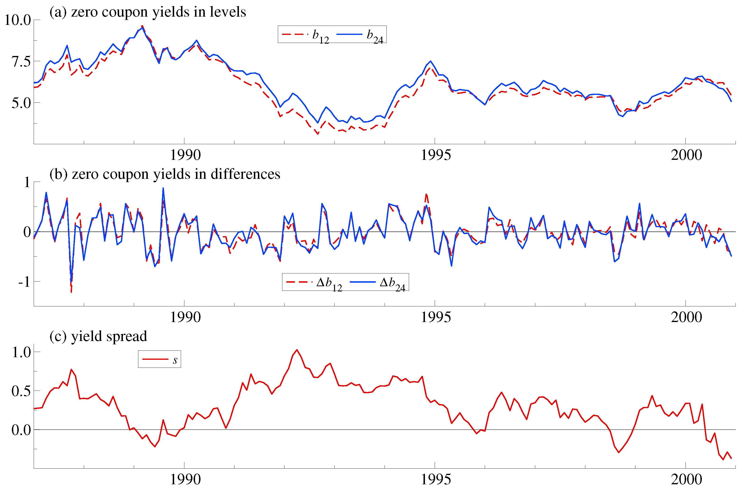
The identification robust inference can be illustrated using a series of monthly US treasury zero-coupon yields over the period 1987:8 to 2000:12. The data are taken from Giese (2008) and runs from the start of Alan Greenspan’s chairmanship of the Fed and finishes before the burst of the dotcom bubble. Giese considers 5 maturities (1, 3, 18, 48, 120 months), but here we only consider 2 maturities (12, 24 months). The empirical analysis uses OxMetrics, see Doornik and Hendry (2013).

Figure 1 shows the data in levels and differences along with the spread. The spread does not appear to have much of a mean reverting behaviour. It is not crossing the long-run average for periods of up to 4 years. This point towards a random walk behaviour which contradicts the expectations hypothesis in line with Giese’s analysis. She finds two common trends among five maturities. The two common trends can be interpreted as short-run and long-run forces driving the yield curve. The cointegrating relations match an extended expectations hypothesis where spreads are not cointegrated but two spreads cointegrate. This is sometimes called butterfly spreads and gives a more flexible match to the yield curve. This is in line with earlier empirical work. Hall et al. (1992), among others, found only one common trend when looking at short-term maturities, while Shea (1992); Zhang (1993) and Carstensen (2003) found more than one common trend when including longer maturities.

Figure 1. Zero coupon yields in (a) levels; (b) differences; and (c) spread.

A vector autoregression of the form (14) with an intercept, $k=4$ lags as well as a dummy variable for 1987:10 was fitted to the data. This has the form

$$\Delta X_t=\Pi X_{t-1}+\mu +\sum _{i=1}^3{\mathsf{\Gamma }}_i\Delta X_{t-i}+\mathsf{\Phi }{1}_{(t=1987:10)}+{\epsilon }_t\mathrm{for}t=1,\cdots ,T,$$

where $X_t$ is the bivariate vector of the 12 and 24 month zero-coupon yields and periods $t=1$ and $t=T$ correspond to 1987:8 and 2000:12 giving $T=161$.

Table 9 reports specification test statistics with p-values in square brackets. The tests do not provide evidence against the initial model. They are the autocorrelation test of Godfrey (1978) the cumulant based normality test, see Doornik and Hansen (2008), and the ARCH test of Engle (1982). For the validity of applying the autoreregressive and normality tests for non-stationarity autoregressions, see Engler and Nielsen (2009), Kilian and Demiroglu (2000), and Nielsen (2006).

Table 9. Specification tests for the unrestricted vector autoregression.

Test	${\mathit{b}}_{12,\mathit{t}}$	${\mathit{b}}_{24,\mathit{t}}$	Test	System
${\chi }_{normality}^2\left(2\right)$	$\underset{[0.15]}{3.8}$	$\underset{[0.13]}{4.1}$	${\chi }_{normality}^2\left(4\right)$	$\underset{[0.36]}{4.3}$
$F_{ar,1-7}\left(7,144\right)$	$\underset{[0.11]}{1.7}$	$\underset{[0.45]}{1.0}$	$F_{ar,1-7}\left(28,272\right)$	$\underset{[0.24]}{1.2}$
$F_{arch,1-7}\left(7,147\right)$	$\underset{[0.09]}{1.8}$	$\underset{[0.41]}{1.0}$

The dummy variable matches the policy intervention after the stock market crash on 19 October 1987. Empirically, the dummy variable can be justified in two ways. First, the plot of yield differences in Figure 1b indicate a sharp drop in yields at that point. Secondly, the robustified least squares algorithm analyzed in Johansen and Nielsen (2016) could be employed for each of the two equations in the model. The algorithm uses a cut-off for outliers in the residuals that is controlled in terms of the gauge, which is the frequency of falsely detected outliers that can be tolerated. The gauge is chosen small in line with recommendations of Hendry and Doornik (2014, Section 7.6), see also Johansen and Nielsen (2016). Thus, we choose a cut-off of 3.02 corresponding to a gauge of 0.25%. When running the autoregressive distributed lag models without outliers, only 1987:10 has an absolute residual exceeding the cut-off. Next, when re-running the model including a dummy for 1987:10, no further residuals exceed the cut-off. This is a fixed point for the algorithm. The detection of outliers may have some impact on specification tests, estimation, and inference. Johansen and Nielsen (2009, 2016) analyze the impact on estimation when the data generating process has no outliers. They find that outlier detection only gives a modest efficiency loss compared to standard least squares when the cut-off is as large as chosen here. Berenguer-Rico and Nielsen (2017) find a considerable impact on the normality test employed above. At present, there is no theory for these algorithms for data generating processes with outliers, albeit some results are available for cointegration analysis with known break date, including the broken trend analysis of Johansen et al. (2000) and the structural change model of Hansen (2003).

Table 10 reports cointegration rank tests. The fifth column shows conventional p-values based on Table 4 and Table 6 for $s=r$ corresponding to Johansen (1995, Tables 15.2, 15.3). The sixth column shows p-values based on Table 5 and Table 6 assuming data have been generating by a model satisfying ${\mathsf{H}}_c(0)={\mathsf{H}}_z(0)$. In both cases the p-values are approximated by fitting a Gamma distribution to the reported mean and variance, see Nielsen (1997); Doornik (1998) for details. As expected, the latter p-values tend to be higher than the former. Overall this provide overwhelming evidence in favour of a pure random walk model in line with Giese (2008).

Table 10. Cointegration rank tests.

Hypothesis	r	Likelihood	$\mathit{LR}$	p-Value
				$\mathit{s}=\mathit{r}$	${\mathsf{H}}_{\mathit{c}}(0)$
${\mathsf{H}}_{c\ell }(2)={\mathsf{H}}_c(2)$	2	134.63
${\mathsf{H}}_{c\ell }(1)$	1	133.71	1.8	0.18	0.39
${\mathsf{H}}_c(1)$	1	133.71	1.8	0.80	0.75
${\mathsf{H}}_{c\ell }(0)$	0	129.70	9.8	0.30	0.46
${\mathsf{H}}_c(0)$	0	129.21	10.8	0.57	0.57

If we have a strong belief in the expectation hypothesis we would, perhaps, ignore the rank tests and seek to test the expectations hypothesis directly. If we maintain the model ${\mathsf{H}}_c(1)$, we could have to contemplate that the cointegration vectors could be nearly unidentified. A mild form of the expectation hypothesis is that the spread is zero mean stationary. Thus, we test the restriction $b^{*}=(1,-1,0)$. The likelihood ratio statistic is 4.0. Assuming the data generating process satisfies either ${\mathsf{H}}_c^{\circ }(0)$ or ${\mathsf{H}}_c^{\circ }(1)$, but not by ${\mathsf{H}}_{c\ell }^{\circ }(0)$, we can apply the Khalaf-Urga (2014)-type bound test established in Theorem 12. The 95% bound in (32) is 14.05 so the hypothesis cannot be rejected based on this test. This contrasts with the above rank tests which gave strong evidence against the expectations hypothesis. The results reconcile if the bounds test does not have much power in the weakly identified case. Indeed, this seems to be the case when looking at Table 3, $\rho =0.99$-panels in Khalaf and Urga (2014), corresponding to near rank deficiency or weak identification. Thus, assuming the rank is one when in fact the data generating process appears to be nearly rank deficient seems to reduce power for tests on the cointegrating vector. That is, when the alleged cointegrating vector is not cointegrating it would be useful to be able to falsify the economic hypothesis. The above mentioned simulations indicate that this is not the case.

5. Conclusions

We have derived asymptotic theory for cointegration rank tests and tests on cointegrating vectors in the rank deficient case. The asymptotic distributions have been simulated and tabulated. The results shed some light on the finite sample theory for cointegration analysis. They can be used to improve the theory on identification robust inference developed by Khalaf and Urga (2014). This was applied to two US treasury yield series.

It appears that large distortions arise when applying standard cointegration inference in the situation where the rank is deficient or nearly deficient. The rank hypothesis gives an inequality for the rank, that is $\mathrm{rank}\Pi \le r$. This includes cases where the rank is r and where it is less than r. Thus, the parameter space for the model where $\mathrm{rank}\Pi \le r$ therefore has a lower dimensional subset where the rank is deficient. Inferential procedures for rank determination are consistent but do leave a positive probability of deciding for a deficient rank in finite samples. In practice, it is therefore possible to end up in a situation of rank deficiency or near deficiency. When proceeding to testing restrictions on the cointegrating vectors, the model is therefore mis-specified or nearly mis-specified.

The asymptotic analysis of the test distributions gives the following results. When testing for cointegration rank, the distribution shifts to the left when the rank is deficient. When testing for restrictions on the cointegrating vector, the distribution shifts to the right when the rank is deficient. When the rank is nearly deficient the distribution will tend to shift in similar directions. As a consequence, a test for cointegration restrictions using conventional critical has a size control problem previously observed by Johansen (2000). One can instead apply identification robust tests as suggested by Khalaf and Urga (2014), but our impression is that while these tests are better behaved in terms of size, they have modest power to reject incorrect restrictions.

Our recommendation is to test for rank before testing restrictions on cointegrating vectors in line with Johansen’s framework. If the conclusion from the rank determination is ambiguous it is best to proceed with caution and possibly explore different choices for rank. This is a common theme in the applied work of Juselius.

References

- Abadir, Karim M. 1995. The limiting distribution of the t ratio under a unit root. Econometric Theory 11: 775–93. [Google Scholar] [CrossRef]
- Andrews, Donald W. K., and Xu Cheng. 2012. Estimation and inference with weak, semi-strong, and strong identification. Econometrica 80: 2153–11. [Google Scholar] [CrossRef]
- Berenguer-Rico, Vanessa, and Bent Nielsen. 2017. Marked and Weighted Empirical Processes of Residuals With Applications to Robust Regressions. Discussion Paper 841. Oxford: Department of Economics, University of Oxford. [Google Scholar]
- Bernstein, David. 2014. Asymptotic Theory for Unidentified Cointegration Estimators. M.Phil. thesis, University of Oxford, Oxford, UK. [Google Scholar]
- Carstensen, Kai. 2003. Nonstationary term premia and cointegration of the term structure. Economics Letters 80: 409–13. [Google Scholar] [CrossRef]
- Cavaliere, Giuseppe, Anders Rahbek, and A. M. Robert Taylor. 2012. Bootstrap determination of the co-integration rank in vector autoregressive models. Econometrica 80: 1721–40. [Google Scholar]
- Doornik, Jurgen A. 1998. Approximations to the asymptotic distribution of cointegration tests. Journal of Economic Surveys 12: 573–93. [Google Scholar] [CrossRef]
- Doornik, Jurgen A. 2007. Object-Oriented Matrix Programming Using Ox, 3rd ed. London: Timberlake. [Google Scholar]
- Doornik, Jurgen A., and Henrik Hansen. 2008. An omnibus test for univariate and multivariate normality. Oxford Bulletin of Economics and Statistics 70: 927–39. [Google Scholar] [CrossRef]
- Doornik, Jurgen A., and David F. Hendry. 2013. PcGive 14. London: Timberlake, vol. 1. [Google Scholar]
- Dufour, Jean-Marie. 1997. Some impossibility theorems in econometrics with applications to structural and dynamic methods. Econometrica 65: 1365–87. [Google Scholar] [CrossRef]
- Engle, Robert F. 1982. Autoregressive conditional heteroscedasticity with estimates of the variance of United Kingdom inflation. Econometrica 50: 987–1108. [Google Scholar] [CrossRef]
- Engler, Eric, and Bent Nielsen. 2009. The empirical process of autoregressive residuals. Econometrics Journal 12: 367–81. [Google Scholar] [CrossRef]
- Fachin, Stefano. 2000. Bootstrap and asymptotic tests of long-run relationships in cointegrated systems. Oxford Bulletin of Economics and Statistics 62: 543–51. [Google Scholar] [CrossRef]
- Giese, Julia. 2008. Level, slope, curvature: Characterising the yield curve in a cointegrated VAR model. Economics 2: 28. [Google Scholar]
- Godfrey, L. G. 1978. Testing against general autoregressive and moving average error models when the regressors include lagged dependent variables. Econometrica 46: 1293–301. [Google Scholar] [CrossRef]
- Gredenhoff, Mikael, and Tor Jacobson. 2001. Bootstrap testing linear restrictions on cointegrating vectors. Journal of Business & Economic Statistics 19: 63–72. [Google Scholar]
- Hall, Anthony D., Heather M. Anderson, and Clive W. J. Granger. 1992. A cointegration analysis of treasury bill yields. Review of Economics and Statistics 74: 116–26. [Google Scholar] [CrossRef]
- Hansen, Peter Reinhard. 2003. Structural changes in the cointegrated vector autoregressive model. Journal of Econometrics 114: 261–95. [Google Scholar] [CrossRef]
- Hendry, David F., and Jurgen A. Doornik. 2014. Empirical Model Discovery and Theory Evaluation: Automatic Selection Methods in Econometrics. London: MIT Press. [Google Scholar]
- Johansen, Søren. 1988. Statistical analysis of cointegration vectors. Journal of Economic Dynamics and Control 12: 231–54. [Google Scholar] [CrossRef]
- Johansen, Søren. 1991. Estimation and hypothesis testing of cointegration vectors in Gaussian vector autoregressive models. Econometrica 59: 1551–580. [Google Scholar] [CrossRef]
- Johansen, Søren. 1992. Determination of cointegration rank in the presence of a linear trend. Oxford Bulletin of Economics and Statistics 54: 383–97. [Google Scholar] [CrossRef]
- Johansen, Søren. 1995. Likelihood Based Inference on Cointegration in the Vector Autoregressive Model. Oxford: Oxford University Press. [Google Scholar]
- Johansen, Søren. 2000. A Bartlett correction factor for tests on the cointegrating relations. Econometric Theory 16: 740–77. [Google Scholar] [CrossRef]
- Johansen, Søren. 2002. A small sample correction of the test for cointegrating rank in the vector autoregressive model. Econometrica 70: 1929–61. [Google Scholar] [CrossRef]
- Johansen, Søren, and Katarina Juselius. 1990. Maximum likelihood estimation and inference on cointegration—With applications to the demand for money. Oxford Bulletin of Economics and Statistics 52: 169–210. [Google Scholar] [CrossRef]
- Johansen, Søren, Rocco Mosconi, and Bent Nielsen. 2000. Cointegration analysis in the presence of structural breaks in the deterministic trend. Econometrics Journal 3: 216–49. [Google Scholar] [CrossRef]
- Johansen, Søren, and Bent Nielsen. 2009. Saturation by indicators in regression models. In The Methodology and Practice of Econometrics: Festschrift in Honour of David F. Hendry. Edited by Jennifer L. Castle and Neil Shephard. Oxford: Oxford University Press, pp. 1–36. [Google Scholar]
- Johansen, Søren, and Bent Nielsen. 2016. Asymptotic theory of outlier detection algorithms for linear time series regression models (with discussion). Scandinavian Journal of Statistics 43: 321–81. [Google Scholar] [CrossRef]
- Juselius, Katarina. 2006. The Cointegrated VAR Model. Oxford: Oxford University Press. [Google Scholar]
- Khalaf, Lynda, and Giovanni Urga. 2014. Identification robust inference in cointegrating regressions. Journal of Econometrics 182: 385–96. [Google Scholar] [CrossRef]
- Kilian, Lutz, and Ufuk Demiroglu. 2000. Residual-based tests for normality in autoregressions: Asymptotic theory and simulation evidence. Journal of Business & Economic Statistics 18: 40–50. [Google Scholar]
- Mavroeidis, Sophocles, Mikkel Plagborg-Møller, and James H. Stock. 2014. Empirical evidence on inflation expectations in the new Keynesian Phillips curve. Journal of Economic Litterature 52: 124–88. [Google Scholar] [CrossRef]
- Nielsen, Bent. 1997. Bartlett correction of the unit root test in autoregressive models. Biometrika 84: 500–504. [Google Scholar] [CrossRef]
- Nielsen, Bent. 1999. The likelihood ratio test for rank in bivariate canonical correlation analysis. Biometrika 86: 279–88. [Google Scholar] [CrossRef]
- Nielsen, Bent. 2001. Conditional test for rank in bivariate canonical correlation analysis. Biometrika 88: 874–80. [Google Scholar] [CrossRef]
- Nielsen, Bent. 2004. On the distribution of likelihood ratio test statistics for cointegration rank. Econometric Reviews 23: 1–23. [Google Scholar] [CrossRef]
- Nielsen, Bent. 2006. Order determination in general vector autoregressions. In Time Series And Related Topics: In Memory of Ching-Zong Wei. Edited by Hwai-Chung Ho, Ching-Kang Ing and Tze Leung Lai. Lecture Notes–Monograph Series; Beachwood: Institute of Mathematical Statistics, vol. 52, pp. 93–112. [Google Scholar]
- Nielsen, Bent, and Anders Rahbek. 2000. Similarity issues in cointegration models. Oxford Bulletin of Economics and Statistics 62: 5–22. [Google Scholar] [CrossRef]
- Paruolo, Paolo. 2001. The power of lambda max. Oxford Bulletin of Economics and Statistics 63: 395–403. [Google Scholar] [CrossRef]
- Phillips, Peter C. B., and Victor Solo. 1992. Asymptotics for linear processes. Annals of Statistics 20: 971–1001. [Google Scholar] [CrossRef]
- Shea, Gary S. 1992. Benchmarking the expectations hypothesis of the interest-rate term structure: An analysis of cointegration vectors. Journal of Business & Economic Statistics 10: 347–366. [Google Scholar]
- Stockmarr, Anders, and Martin Jacobsen. 1994. Gaussian diffusion and autoregressive processes: Weak convergence and statistical inference. Scandinavian Journal of Statistics 21: 403–19. [Google Scholar]
- Swensen, Anders Rygh. 2004. Bootstrap algorithms for testing and determining the cointegration rank in VAR models. Econometrica 74: 1699–714, Corrigendum in volume 77: 1703–704. [Google Scholar] [CrossRef]
- Zhang, Hua. 1993. Treasury yield curves and cointegration. Applied Economics 25: 361–67. [Google Scholar] [CrossRef]
© 2019 by the authors. Licensee MDPI, Basel, Switzerland. This article is an open access article distributed under the terms and conditions of the Creative Commons Attribution (CC BY) license (http://creativecommons.org/licenses/by/4.0/).