Using the GB2 Income Distribution

Abstract

To use the generalized beta distribution of the second kind (GB2) for the analysis of income and other positively skewed distributions, knowledge of estimation methods and the ability to compute quantities of interest from the estimated parameters are required. We review estimation methodology that has appeared in the literature, and summarize expressions for inequality, poverty, and pro-poor growth that can be used to compute these measures from GB2 parameter estimates. An application to data from China and Indonesia is provided.

1. Introduction

Specification and estimation of parametric income distributions has a long history in economics. Much of the literature on alternative distributions can be accessed through the book by Kleiber and Kotz (2003), and the papers in Chotikapanich (2008). A series of papers by McDonald and his coauthors (McDonald 1984; McDonald and Xu 1995; Bordley et al. 1997; McDonald and Ransom 2008; McDonald et al. 2011) carry details of many of the distributions and the relationships between them. Our focus in this paper is on the generalized beta distribution of the second kind (GB2). It is a four-parameter distribution defined over the support $(0,\infty )$, and obtained by transforming a standard beta random variable defined on $(0,\hspace{0.17em}1).$ As described by McDonald and Xu (1995), it nests many popular three-parameter specifications of income distributions including the generalized gamma, beta2, Singh-Maddala and Dagum distributions. Two-parameter special cases of these distributions include the lognormal, gamma, Weibull, Lomax and Fisk distributions.1 Parker (1999) describes a model of firm optimizing behavior that leads to a GB2 distribution for earnings. Applications have appeared in Butler and McDonald (1986), Cummins et al. (1990), Feng et al. (2006), Jenkins (2009), Graf and Nedyalkova (2014), and Jones et al. (2014). Biewen and Jenkins (2005) analyze poverty differences using Singh-Maddala and Dagum distributions, with parameters as functions of personal household characteristics, and with their choice between the Singh-Maddala and Dagum distributions based on preliminary estimates of GB2 distributions. Quintano and D’Agostino (2006) use the Dagum distribution and the Biewen-Jenkins methodology to examine the dependence of inequality and poverty on personal characteristics. In an extensive study examining global inequality, Chotikapanich et al. (2012) estimate special case beta2 distributions for 91 countries in 1993 and 2000. In an application involving 10 regions, Hajargasht and Griffiths (2013) find that the GB2 distribution compares favorably with the four-parameter double Pareto-lognormal distribution in terms of goodness-of-fit.

Estimation of a good-fitting parametric income distribution such as the GB2 facilitates further analysis. Once important quantities such as mean income, the Gini coefficient, the Lorenz curve, and the headcount ratio have been expressed in terms of the parameters of the distribution, they can be readily estimated from those parameters. If interest centers on a region which comprises a collection of countries or areas, a GB2 distribution can be estimated for each country/area; inequality, poverty and pro-poor growth for the region can be analyzed by computing estimates of indicators expressed in terms of the parameters of a regional distribution which will be a population-weighted mixture of the GB2 distributions. If only grouped data are available, then estimating a distribution such as the GB2 provides a means for accommodating within-group variation, an important consideration for assessing inequality and poverty.

The purpose of this paper is to collect results on measures for inequality, poverty, and pro-poor growth, expressed as functions of the parameters of the GB2 distribution and its mixtures, and to summarize various methods of estimation that have appeared in the literature for estimating GB2 parameters from single observations or from grouped data. Expressions for the inequality, poverty, and pro-poor growth measures are given in Section 2. Section 3 contains a description of the various estimation techniques. The results from an application to 4 years of data for China and Indonesia are presented in Section 4. Some concluding remarks are offered in Section 5.

2. Inequality and Poverty Measures from the GB2 Distribution

Throughout we assume that income $Y$ for a given country or area, can be represented by a GB2 distribution whose probability density function (pdf) is given by

$$f\left(y|a,b,p,q\right)=\frac{a{y}^{ap-1}}{b^{ap}\mathrm{B}(p,q){\left(1+{\left(\frac{y}{b}\right)}^a\right)}^{p+q}}\hspace{1em}\hspace{1em}y>0$$

(1)

where $a>0,\hspace{0.17em}\hspace{0.17em}b>0,\hspace{0.17em}\hspace{0.17em}p>0 \mathrm{and} q>0$ are its parameters and $\mathrm{B}(p,q)\hspace{0.17em}={\displaystyle {\int }_0^1{t}^{p-1}{(1-t)}^{q-1}dt}$ is the beta function. The cumulative distribution function (cdf) corresponding to (1) is given by

$$F(y|a,b,p,q)=\frac{1}{\mathrm{B}(p,q)}{\displaystyle \underset{0}{\overset{w}{\int }}\hspace{0.17em}\hspace{0.17em}{t}^{p-1}{(1-t)}^{q-1}dt}=B\left(w|p,q\right)$$

(2)

where $w={\left(y/b\right)}^a/\left[1+{\left(y/b\right)}^a\right]$. The function $B(w|p,q)$ is the cdf for the normalized beta distribution, defined on the (0, 1) interval, with parameters $p$ and $q,$ and evaluated at $w$. It is a convenient representation because both it, and its inverse, are commonly included as readily-computed functions in statistical software. Properties of the GB2 distribution and its special cases have been considered extensively by McDonald (1984) and Kleiber and Kotz (2003). Three-parameter special cases, which have been popular in the literature, are the Singh-Maddala distribution2 where $p=1,$ the Dagum distribution where $q=1,$ and the beta2 distribution where $a=1$. Extension to a 5-parameter GB distribution has been considered by McDonald and Xu (1995) and McDonald and Ransom (2008). Some further properties of the GB2 distribution are described by Graf and Nedyalkova (2014). In this section, we summarize the main results from the GB2 distribution that are relevant for computing measures of inequality, poverty and pro-poor growth.

We envisage a scenario where GB2 distributions have been estimated for a number of countries, or for specific areas within a country such as urban and rural, and the objective is to evaluate inequality and poverty measures using the estimated parameters of the GB2 distributions. As well as evaluation of the measures from single GB2 distributions, we are interested in evaluating them for mixtures that arise when urban and rural GB2 distributions are combined to obtain a distribution for a country, or when country GB2 distributions are combined to obtain the distribution for a region. In most instances, we can express measures in terms of quantities such as beta and gamma functions that are readily computed by available software. Measures whose exact computation proves to be difficult can usually be written in terms of expectations which can be estimated by averaging values of the function over simulated draws from one or more of the GB2 distributions. Key quantities that are used for calculation of many measures, and for estimation of GB2 distributions, are the GB2 moments and moment distribution functions. We begin by giving expressions for them, as well as indicating how the GB2 Lorenz curve can be obtained. We then consider measures for inequality, poverty and pro-poor growth.

The $k$-th moment of the GB2 exists for $-ap<k<aq$ and is given by

$$\begin{array}{ll}{\mathsf{\mu }}^{(k)}=E\left(Y^k\right)& =\frac{b^k\mathrm{B}\left(p+k/a,q-k/a\right)}{\mathrm{B}\left(p,q\right)}\\ & =\frac{b^k\Gamma \left(p+k/a\right)\Gamma \left(q-k/a\right)}{\Gamma (p)\Gamma (q)}\end{array}$$

(3)

where $\Gamma (\cdot )$ is the gamma function. The $k$-th moment distribution function for the GB2 is given by3

$$\begin{array}{ll}{F}_k\left(y|a,b,p,q\right)& =\frac{1}{{\mathsf{\mu }}^{(k)}}{\displaystyle \underset{0}{\overset{y}{\int }}{t}^{k}f\left(t\right)dt}\\ & =F\left(y|a,b,p+k/a,q-k/a\right)\end{array}$$

This result—that the GB2’s moment distribution functions can be written in terms of its cdf evaluated at different parameter values—is particularly useful for deriving the Lorenz curve and for setting up and computing GMM estimates from grouped data. The Lorenz curve, relating the cumulative proportion of income $\mathsf{\eta }$ to the cumulative proportion of population $u$ is given by

$$\begin{array}{ll}\mathsf{\eta }(u)& =F_1\left[F^{-1}\left(u|a,b,p,q\right)|a,b,p,q\right]\\ & =F\left[F^{-1}\left(u|a,b,p,q\right)|a,b,p+1/a,q-1/a\right]\\ & =B\left[B^{-1}\left(u|p,q\right)|p+1/a,q-1/a\right]\hspace{1em}\hspace{1em}\hspace{1em}\hspace{1em}0<u<1\end{array}$$

where the function $B\left(\cdot |\cdot ,\cdot \right)$ is defined in Equation (2).

2.1. Inequality Measures

2.1.1. Gini Coefficient

The most widely used inequality measure is the Gini coefficient. McDonald (1984) and McDonald and Ransom (2008) use hypergeometric functions to express the Gini coefficient in terms of the GB2 parameters. An algorithm for computing these functions has been proposed by Graf (2009). It has been our experience that it is easier computationally to compute the Gini coefficient via numerical integration than to numerically evaluate the hypergeometric functions. Another alternative is to estimate the Gini coefficient by simulating from the GB2 distribution. Specifically, noting that the Gini coefficient is given by

$$\begin{array}{ll}G& =-1+\frac{2}{\mathsf{\mu }}{\displaystyle \underset{0}{\overset{\infty }{\int }}yF\left(y|\mathsf{\varphi }\right)}f\left(y|\mathsf{\varphi }\right)dy\\ & =-1+\frac{2}{\mathsf{\mu }}E\left[yF\left(y|\mathsf{\varphi }\right)\right]\end{array}$$

where $\mathsf{\mu }={\mathsf{\mu }}^{(1)}=E\left(y\right)=b\left[\Gamma \left(p+1/a\right)\Gamma \left(q-1/a\right)\right]/\left[\Gamma (p)\Gamma (q)\right]$ and ${\mathsf{\varphi }}^{\prime }=\left(a,b,p,q\right),$ we can draw observations $\left(y_1,y_2,\dots ,y_M\right)$ from $f\left(y|\mathsf{\varphi }\right)$ and estimate $G$ from

$$\widehat{G}=-1+\frac{2}{\mathsf{\mu }}\frac{1}{M}{\displaystyle \sum _{m=1}^M{y}_{m}F\left(y_m|\mathsf{\varphi }\right)}$$

The number of draws $M$ can be made as large as necessary to achieve the derived level of accuracy. To draw observations from $f\left(y|\mathsf{\varphi }\right)$, we first draw observations $\left(w_1,w_2,\dots ,w_M\right)$ from a standard beta $(p,q)$ distribution, defined on the $(0,\hspace{0.17em}1)$ interval, and then compute $y_m=b{\left[w_m/\left(1-w_m\right)\right]}^{1/a}.$ If interest centers on one of the special case distributions where $p=1,$ $q=1$ or $a=1,$ then closed form expressions in terms of gamma or beta functions are available for the Gini coefficient. They are

$$\mathrm{Beta}2\hspace{1em}\hspace{1em}a=1\hspace{1em}\hspace{1em}G=\frac{2\mathsf{{\rm B}}\left(2p,2q-1\right)}{2{\mathsf{{\rm B}}}^2\left(p,q\right)}$$

$$\begin{gathered} \text{Singh–Maddala}\hspace{1em}\hspace{1em}p=1\hspace{1em}\hspace{1em}G=1-\frac{\Gamma \left(q\right)\Gamma \left(2q-1/a\right)}{\Gamma \left(q-1/a\right)\Gamma \left(2q\right)} \\ \mathrm{Dagum}\hspace{1em}\hspace{1em}q=1\hspace{1em}\hspace{1em}G=\frac{\Gamma \left(p\right)\Gamma \left(2p+1/a\right)}{\Gamma \left(2p\right)\Gamma \left(p+1/a\right)}-1 \end{gathered}$$

Suppose now we have estimated GB2 income distributions for a number of different areas, such as countries within a region or urban and rural areas within a country, and we are interested in estimating the Gini coefficient for the combined area. The combined income distribution can be written as a population-weighted mixture of the individual GB2 distributions. That is,

$$f\left(y|\mathsf{\Phi }\right)={\displaystyle \sum _{j=1}^J{\lambda }_{j}f\left(y|{\mathsf{\varphi }}_j\right)}$$

(4)

where $\mathsf{\Phi }=\left({\mathsf{\varphi }}_1,{\mathsf{\varphi }}_2,\dots ,{\mathsf{\varphi }}_J\right)$, ${\lambda }_j$ is the proportion of the combined population in area $j,$ and ${{\mathsf{\varphi }}^{\prime }}_j=\left(a_j,b_j,p_j,q_j\right)$ is the vector of parameters of the distribution for area j. As noted by Chotikapanich et al. (2007), in this case the Gini coefficient for a combination of $J$ areas can be estimated from

$$G=-1+\frac{2}{{\mathsf{\mu }}_C}{\displaystyle \sum _{j=1}^J{\displaystyle \sum _{\ell =1}^J{\lambda }_j{\lambda }_{\ell }{\mathsf{\tau }}_{j\ell }}}$$

where

$${\mathsf{\tau }}_{j\ell }=\frac{1}{M}{\displaystyle \sum _{m=1}^M{y}_{j,m}F\left(y_{j,m}|{\mathsf{\varphi }}_{\ell }\right)}$$

${\mathsf{\mu }}_C={\displaystyle {\sum }_{j=1}^J{\lambda }_j{\mathsf{\mu }}_j}$ is the mean of the combined areas, ${\mathsf{\mu }}_j$ is the mean for area $j,$ and $y_{j,m}$ is the $m$-th draw from pdf $f\left(y|{\mathsf{\varphi }}_j\right).$ For the empirical work in this paper we estimated separate distributions for rural and urban areas in China and Indonesia, then combined them.

2.1.2. Generalized Entropy Measures

Next we consider the generalized entropy (GE) class of inequality measures, whose expressions in terms of the parameters of the GB2 distribution were provided by Jenkins (2009). The GE index is given by

$$I(\mathsf{\alpha })=\frac{1}{\mathsf{\alpha }\left(\mathsf{\alpha }-1\right)}\left[\frac{{\mathsf{\mu }}^{(\mathsf{\alpha })}}{{\mathsf{\mu }}^{\mathsf{\alpha }}}-1\right]\hspace{1em}\hspace{1em}\hspace{1em}\hspace{1em}\hspace{1em}\hspace{1em}\mathrm{for} \mathsf{\alpha }\ne 0,1$$

(5)

where, for the GB2 distribution, ${\mathsf{\mu }}^{(\mathsf{\alpha })}={\displaystyle {\int }_0^{\infty }{y}^{\mathsf{\alpha }}f(y|\mathsf{\varphi })dy}$ is given in (3), and ${\mathsf{\mu }}^{\mathsf{\alpha }}={\left[{\mathsf{\mu }}^{(1)}\right]}^{\mathsf{\alpha }}$. For large positive $\mathsf{\alpha },$ the index $I\left(\mathsf{\alpha }\right)$ is sensitive to large differences at the top of the distribution; for large negative $\mathsf{\alpha },$ it is sensitive to differences at the bottom end of the distribution. Theoretically, $\mathsf{\alpha }$ can range from $-\infty$ to $\infty$, but values between −1 and 2 are usually considered in applications. Two popular special cases are obtained by taking limits as $\mathsf{\alpha }\to 0$ and $\mathsf{\alpha }\to 1$. The case where $\mathsf{\alpha }\to 0$ is known as the mean logarithmic deviation or Theil(0) (Theil 1967, p. 127). Its general expression, and the result for the GB2 distribution, are4

$$\begin{array}{ll}I(0)& ={\displaystyle \underset{0}{\overset{\infty }{\int }}\log \left(\frac{\mathsf{\mu }}{y}\right)f\left(y|\mathsf{\varphi }\right)dy}\\ & =\log (\mathsf{\mu })-E\left[\log (y)\right]\\ & =\ln \left(\mathsf{\mu }/b\right)-\mathsf{\psi }(p)/a+\mathsf{\psi }(q)/a\end{array}$$

where $\mathsf{\psi }(c)=d\log \Gamma (c)/dc$ is the digamma function, computable by most software. The index obtained as $\mathsf{\alpha }\to 1$ is known as Theil(1) (Theil 1967, p. 96). Its general expression, and result for the GB2 distribution, are

$$\begin{array}{ll}I(1)& ={\displaystyle \underset{0}{\overset{\infty }{\int }}\frac{y}{\mathsf{\mu }}\log \left(\frac{y}{\mathsf{\mu }}\right)f(y|\mathsf{\varphi })dy}\\ & =\left[E\left(y\log (y)\right)\right]/\mathsf{\mu }-\log \mathsf{\mu }\\ & =\left[\mathsf{\psi }\left(p+1/a\right)-\mathsf{\psi }\left(q-1/a\right)\right]/a+\log \left(b/\mathsf{\mu }\right)\end{array}$$

In the event that software is not available to compute the digamma function, draws $\left(y_1,y_2,\dots ,y_M\right)$ from $f\left(y|\mathsf{\varphi }\right)$ can be used to calculate ${\displaystyle {\sum }_{m=1}^M\log \left(y_m\right)}/M$ and ${\displaystyle {\sum }_{m=1}^M{y}_m\log \left(y_m\right)}/M$ as estimators for $E\left[\log (y)\right]$ and $E\left[y\log (y)\right]$, respectively.

The GE index for a mixture of income distributions and its decomposition into within and between group inequality has been considered by Sarabia et al. (2017). To obtain the GE index for a region whose income distribution is a mixture of GB2 distributions, the quantities ${\mathsf{\mu }}^{(\mathsf{\alpha })}$ and ${\mathsf{\mu }}^{\mathsf{\alpha }},$ defined in (5) for the GB2 distribution $f\left(y|\mathsf{\varphi }\right),$ are replaced by the corresponding moments for the mixture distribution $f\left(y|\mathsf{\Phi }\right)={\displaystyle {\sum }_{j=1}^J{\lambda }_{j}f\left(y|{\mathsf{\varphi }}_j\right)}$ given in (4). For $\mathsf{\alpha }\ne 0,\hspace{0.17em}1,$ the resulting index is

$$\begin{array}{ll}{I}_C(\mathsf{\alpha })& =\frac{1}{\mathsf{\alpha }\left(\mathsf{\alpha }-1\right)}\left[{\displaystyle \underset{0}{\overset{\infty }{\int }}{\left(\frac{y}{{\mathsf{\mu }}_C}\right)}^{\mathsf{\alpha }}{\displaystyle \sum _{j=1}^J{\lambda }_{j}f\left(y|{\mathsf{\varphi }}_j\right)dy}}-1\right]\\ & =\frac{1}{\mathsf{\alpha }\left(\mathsf{\alpha }-1\right)}\left[\frac{1}{{\mathsf{\mu }}_C^{\mathsf{\alpha }}}{\displaystyle \sum _{j=1}^J{\lambda }_j{E}_j\left(y^{\mathsf{\alpha }}\right)}-1\right]\\ & =\frac{1}{\mathsf{\alpha }\left(\mathsf{\alpha }-1\right)}\left[\frac{{\displaystyle {\sum }_{j=1}^J{\lambda }_j{\mathsf{\mu }}_j^{(\mathsf{\alpha })}}}{{\left({\displaystyle {\sum }_{j=1}^J{\lambda }_j{\mathsf{\mu }}_j}\right)}^{\mathsf{\alpha }}}-1\right]\end{array}$$

(6)

where ${\mathsf{\mu }}_j^{(\mathsf{\alpha })}=E_j\left(y^{\mathsf{\alpha }}\right)$ is the $\mathsf{\alpha }$-moment with respect to $f\left(y|{\mathsf{\varphi }}_j\right)$, the distribution of the $j$-th component. For the case where $\mathsf{\alpha }=0,$ we have

$$\begin{array}{ll}{I}_C(0)& ={\displaystyle \underset{0}{\overset{\infty }{\int }}\log \left(\frac{{\mathsf{\mu }}_C}{y}\right){\displaystyle \sum _{j=1}^J{\lambda }_{j}f\left(y|{\mathsf{\varphi }}_j\right)dy}}\\ & =\log {\mathsf{\mu }}_C-{\displaystyle \sum _{j=1}^J{\lambda }_j{E}_j\left(\log y\right)}\end{array}$$

where, for the GB2 distribution, $E_j\left(\log y\right)=\left[\mathsf{\psi }\left(p_j\right)-\mathsf{\psi }\left(q_j\right)\right]/a_j+\log \left(b_j\right)$. For the case where $\mathsf{\alpha }=1$,

$$\begin{array}{ll}{I}_C(1)& ={\displaystyle \underset{0}{\overset{\infty }{\int }}\frac{y}{{\mathsf{\mu }}_C}\log \left(\frac{y}{{\mathsf{\mu }}_C}\right){\displaystyle \sum _{j=1}^J{\lambda }_{j}f\left(y|{\mathsf{\varphi }}_j\right)dy}}\\ & =\frac{1}{{\mathsf{\mu }}_C}{\displaystyle \sum _{j=1}^J{\lambda }_j{E}_j\left(y\log y\right)}-\log {\mathsf{\mu }}_C\end{array}$$

with

$$E_j\left(y\log y\right)=\left({\mathsf{\mu }}_j/a_j\right)\left[\mathsf{\psi }\left(p_j+1/a_j\right)-\mathsf{\psi }\left(q_j-1/a_j\right)\right]+{\mathsf{\mu }}_j\log b_j.$$

An attractive feature of the GE index from a mixture is that it decomposes into a GE measure of inequality within the components of the mixture and a GE measure of inequality between components. To establish this decomposition, we write the index for the j-th area as

$$I_j(\mathsf{\alpha })=\frac{1}{\mathsf{\alpha }\left(\mathsf{\alpha }-1\right)}\left[\frac{{\mathsf{\mu }}_j^{(\mathsf{\alpha })}}{{\mathsf{\mu }}_j^{\mathsf{\alpha }}}-1\right]$$

and note that

$$\frac{{\mathsf{\mu }}_j^{(\mathsf{\alpha })}}{{\mathsf{\mu }}_j^{\mathsf{\alpha }}}=\mathsf{\alpha }(\mathsf{\alpha }-1)I_j(\mathsf{\alpha })+1$$

Substituting this expression into (6) yields

$$\begin{array}{ll}{I}_C(\mathsf{\alpha })& =\frac{1}{\mathsf{\alpha }\left(\mathsf{\alpha }-1\right)}\left\{{\displaystyle \sum _{j=1}^J{\lambda }_j{\left(\frac{{\mathsf{\mu }}_j}{{\mathsf{\mu }}_C}\right)}^{\mathsf{\alpha }}}\left[\mathsf{\alpha }\left(\mathsf{\alpha }-1\right)I_j(\mathsf{\alpha })\hspace{0.17em}+1\right]\hspace{0.17em}-\hspace{0.17em}1\right\}\\ & ={\displaystyle \sum _{j=1}^J{\lambda }_j{\left(\frac{{\mathsf{\mu }}_j}{{\mathsf{\mu }}_C}\right)}^{\mathsf{\alpha }}{I}_j(\mathsf{\alpha })}+\frac{1}{\mathsf{\alpha }\left(\mathsf{\alpha }-1\right)}\left\{{{\displaystyle \sum _{j=1}^J{\lambda }_j\left(\frac{{\mathsf{\mu }}_j}{{\mathsf{\mu }}_C}\right)}}^{\mathsf{\alpha }}-1\right\}\\ & =I_C^{with}(\mathsf{\alpha })+I_C^{betw}(\mathsf{\alpha })\end{array}$$

where $I_C^{with}(\mathsf{\alpha })={\displaystyle {\sum }_{j=1}^J{\lambda }_j{\left({\mathsf{\mu }}_j/{\mathsf{\mu }}_C\right)}^{\mathsf{\alpha }}{I}_j\left(\mathsf{\alpha }\right)}$ is a weighted average of the inequalities for each area with weights given by ${\lambda }_j{\left({\mathsf{\mu }}_j/{\mathsf{\mu }}_C\right)}^{\mathsf{\alpha }}$, and $I_C^{betw}(\mathsf{\alpha })={\left[\mathsf{\alpha }\left(\mathsf{\alpha }-1\right)\right]}^{-1}\left\{{\displaystyle {\sum }_{j=1}^J{\lambda }_j{\left({\mathsf{\mu }}_j/{\mathsf{\mu }}_C\right)}^{\mathsf{\alpha }}-1}\right\}$ is a discrete version of the GE index for the J areas, measuring between inequality. Note that, unless $\mathsf{\alpha }=0$ or 1, the weights do not sum to 1. When $\mathsf{\alpha }=0$, the weights are the population shares ${\lambda }_j$; when $\mathsf{\alpha }=1$, the weights are the income shares ${\lambda }_j{\mathsf{\mu }}_j/{\displaystyle {\sum }_{j=1}^J{\lambda }_j{\mathsf{\mu }}_j}$. The components for these two cases are

$$\begin{array}{ll}{I}_C^{with}\left(0\right)& ={\displaystyle \sum _{j=1}^J{\lambda }_j{I}_j(0)}\\ & ={\displaystyle \sum _{j=1}^J{\lambda }_j\log \left({\mathsf{\mu }}_j\right)-{\displaystyle \sum _{j=1}^J{\lambda }_j{E}_j\left(\log y\right)}}\end{array}$$

$$\begin{gathered} \begin{array}{ll}{I}_C^{betw}(0)& ={\displaystyle \sum _{j=1}^J{\lambda }_j\log \left(\frac{{\mathsf{\mu }}_C}{{\mathsf{\mu }}_j}\right)}\\ & =\log {\mathsf{\mu }}_C-{\displaystyle \sum _{j=1}^J{\lambda }_j\log {\mathsf{\mu }}_j}\end{array} \\ \begin{array}{ll}{I}_C^{with}\left(1\right)& ={\displaystyle \sum _{j=1}^J{\lambda }_j\frac{{\mathsf{\mu }}_j}{{\mathsf{\mu }}_C}{I}_j(1)}\\ & =\frac{1}{{\mathsf{\mu }}_C}{\displaystyle \sum _{j=1}^J{\lambda }_j{E}_j\left(y\log y\right)-{\displaystyle \sum _{j=1}^J{\lambda }_j\frac{{\mathsf{\mu }}_j}{{\mathsf{\mu }}_C}\log \left({\mathsf{\mu }}_j\right)}}\end{array} \\ \begin{array}{ll}{I}_C^{betw}\left(1\right)& ={\displaystyle \sum _{j=1}^J{\lambda }_j\frac{{\mathsf{\mu }}_j}{{\mathsf{\mu }}_C}\log \left(\frac{{\mathsf{\mu }}_j}{{\mathsf{\mu }}_C}\right)}\\ & ={\displaystyle \sum _{j=1}^J{\lambda }_j\frac{{\mathsf{\mu }}_j}{{\mathsf{\mu }}_C}\log \left({\mathsf{\mu }}_j\right)}-\log {\mathsf{\mu }}_C\end{array} \end{gathered}$$

2.1.3. Atkinson Index

The Atkinson index is an inequality index that can be viewed as an ordinal special case of a GE index. It is given by

$$A(\mathsf{\epsilon })=1-\frac{1}{\mathsf{\mu }}{\left[{\mathsf{\mu }}^{(1-\mathsf{\epsilon })}\right]}^{1/\left(1-\mathsf{\epsilon }\right)}\hspace{1em}\hspace{1em}\hspace{1em}\hspace{1em}\hspace{1em}\mathrm{for} 0<\mathsf{\epsilon }\ne 1$$

$$A(1)=1-\frac{\exp \left\{E\left(\log (y)\right)\right\}}{\mathsf{\mu }}$$

The parameter $\mathsf{\epsilon }$ reflects the degree of aversion to inequality in a social welfare function. As $\mathsf{\epsilon }\to 0,$ there is no aversion to inequality, and $A(\mathsf{\epsilon })\to 0$. As $\mathsf{\epsilon }\to \infty ,$ social welfare is increased by redistributing income towards complete equality; $A(\mathsf{\epsilon })\to 1$. To compute $A$ from the parameters of the GB2 distribution, we note that ${\mathsf{\mu }}^{(1-\mathsf{\epsilon })}$ is given in Equation (3) and $E\left[\log (y)\right]=\left[\mathsf{\psi }(p)-\mathsf{\psi }(q)\right]/a-\log (b).$ Alternatively, and for computing $A_C(\mathsf{\epsilon }),$ the Atkinson index for a mixture of GB2 distributions, the relationship between $A(\mathsf{\epsilon })$ and the GE index $I(\mathsf{\alpha })$ can be exploited. With $\mathsf{\alpha }=1-\mathsf{\epsilon },$ and $\mathsf{\epsilon }>0,$ it is given by

$$A(\mathsf{\epsilon })=1-{\left[\mathsf{\alpha }(\mathsf{\alpha }-1)I(\mathsf{\alpha })+1\right]}^{1/\mathsf{\alpha }}\hspace{1em}\hspace{1em}\hspace{1em}\hspace{1em}\hspace{1em}\mathrm{for} 0\ne \mathsf{\alpha }<1$$

$$A(0)=1-\exp \left\{-I(0)\right\}$$

2.1.4. Pietra Index

In contrast to the Gini coefficient, which is equal to twice the area between the Lorenz curve and the line of perfect equality, the Pietra index is equal to the maximum distance between the Lorenz curve and the perfect equality line (Kleiber and Kotz 2003), as well as twice the area of the largest triangle within the area between the Lorenz curve and line of perfect equality (Butler and McDonald 1989). Details of these results and an extensive analysis of the Pietra index, generally, and in terms of several distributions and their mixtures, can be found in Sarabia and Jordá (2014). For a single GB2 distribution, we have

$$\begin{array}{ll}P& =\frac{1}{2\mathsf{\mu }}{\displaystyle \underset{0}{\overset{\infty }{\int }}\left|y-\mathsf{\mu }\right|f\left(y|\mathsf{\varphi }\right)dy}\\ & =F\left(\mathsf{\mu }|\mathsf{\varphi }\right)-F_1\left(\mathsf{\mu }|\mathsf{\varphi }\right)\\ & =F\left(\mathsf{\mu }|a,b,p,q\right)-F\left(\mathsf{\mu }|a,b,p+1/a,q-1/a\right)\end{array}$$

For a mixture of distributions, it is given by

$$P_C={\displaystyle \sum _{j=1}^J{\lambda }_{j}F\left({\mathsf{\mu }}_C|{\mathsf{\varphi }}_j\right)-\frac{1}{{\mathsf{\mu }}_C}{\displaystyle \sum _{j=1}^J{\lambda }_j{\mathsf{\mu }}_j{F}_1\left({\mathsf{\mu }}_C|{\mathsf{\varphi }}_j\right)}}$$

2.1.5. Quintile Share Ratio

Inequality is often also expressed in terms of the ratio of the income share of the richest to the income share of the poorest in the population. Graf and Nedyalkova (2014) consider the quintile share ratio ($QSR$), which is the ratio of the income share of the richest 20% relative to the income share of the poorest 20%. For the GB2 distribution, it is given by

$$QSR=\frac{1-B\left[B^{-1}\left(0.8|p,q\right)|p+1/a,q-1/a\right]}{B\left[B^{-1}\left(0.2|p,q\right)|p+1/a,q-1/a\right]}$$

Noting that,

$$\begin{array}{ll}{F}_1\left(y|\mathsf{\Phi }\right)& =\frac{1}{{\mathsf{\mu }}_C}{\displaystyle \underset{0}{\overset{y}{\int }}t{\displaystyle \sum _{j=1}^J{\lambda }_{j}f\left(t|{\mathsf{\varphi }}_j\right)dt}}\\ & =\frac{1}{{\mathsf{\mu }}_C}{\displaystyle \sum _{j=1}^J{\lambda }_j{\mathsf{\mu }}_j{F}_1\left(y|{\mathsf{\varphi }}_j\right)}\end{array}$$

the $QSR$ for a mixture of GB2 distributions can be computed from

$$QS{R}_C=\frac{1-{\displaystyle \sum _{j=1}^J{\lambda }_j{\mathsf{\mu }}_{j}B\left(w_{j,0.8}|p_j+1/a_j,q_j-1/a_j\right)}}{{\displaystyle \sum _{j=1}^J{\lambda }_j{\mathsf{\mu }}_{j}B\left(w_{j,0.2}|p_j+1/a_j,q_j-1/a_j\right)}}$$

where $w_{j,0.8}={\left(y_{0.8}/b_j\right)}^{a_j}/\left[1+{\left(y_{0.8}/b_j\right)}^{a_j}\right]$ and $w_{j,0.2}={\left(y_{0.2}/b_j\right)}^{a_j}/\left[1+{\left(y_{0.2}/b_j\right)}^{a_j}\right],$ with $y_{0.2}$ and $y_{0.8}$ being the 20th and 80th percentiles from the mixture distribution. To obtain $y_{0.2}$ and $y_{0.8}$, the mixture distribution function needs to be inverted to obtain its corresponding quantile function, something that is not possible in closed form. As alternatives, one can (1) attempt to solve the required equation numerically, or (2) generate a large number of observations from each component, combine and sort these components, choosing the 20th and 80th empirical percentiles as estimates.

2.2. Poverty Measures

Expressions for several poverty measures in terms of the parameters of the GB2 distribution have been provided by Chotikapanich et al. (2013). The first is the headcount ratio which is simply the proportion of the population with income less than or equal to a poverty line $z$

$$H(z)=F\left(z|\mathsf{\varphi }\right)=B\left(v|p,q\right)$$

(7)

where $v={\left(z/b\right)}^a/\left[1+{\left(z/b\right)}^a\right].$ Setting the poverty line at 0.6 times the median gives what Graf and Nedyalkova (2014) term the at-risk-poverty rate ($ARPR$). It can be calculated from (7) after setting the poverty line at

$$z=0.6b{\left(\frac{B^{-1}\left(0.5|p,q\right)}{1-B^{-1}\left(0.5|p,q\right)}\right)}^{1/a}$$

(8)

A second poverty measure used extensively in the literature is the $FGT(\mathsf{\alpha })$ class of measures (Foster et al. 1984) given by

$$FGT(\mathsf{\alpha })={\displaystyle \underset{0}{\overset{z}{\int }}{\left(\frac{z-y}{z}\right)}^{\mathsf{\alpha }}f\left(y|\mathsf{\varphi }\right)dy}\hspace{1em}\hspace{1em}\hspace{1em}\mathrm{for} \mathsf{\alpha }\ge 1$$

For integer values of $\mathsf{\alpha },$ this expression can be written in terms of incomplete moments of the GB2 distribution as well as in terms of the income gap ratio, defined as the average amount of money that must be given to each of the poor to bring them up to the poverty line, expressed relative to the poverty line. Working in this direction, we define the $k$-th incomplete moment for the GB2 distribution, relative to poverty line z, as

$$\begin{array}{ll}{\mathsf{\mu }}_z^{(k)}& =E\left(y^k|y<z\right)=\frac{1}{F\left(z|\mathsf{\varphi }\right)}{\displaystyle \underset{0}{\overset{z}{\int }}{y}^{k}f\left(y|\mathsf{\varphi }\right)dy}\\ & =\frac{{\mathsf{\mu }}^{(k)}B\left(v|p+k/a,q-k/a\right)}{B\left(v|p,q\right)}\end{array}$$

Defining the income gap ratio as $g(z)=\left(z-{\mathsf{\mu }}_z\right)/z$ where ${\mathsf{\mu }}_z={\mathsf{\mu }}_z^{(1)}$ is mean income of the poor, we can write

$$\begin{array}{ll}FGT(1)& =B\left(v|p,q\right)-\left(\mathsf{\mu }/z\right)B\left(v|p+1/a,q-1/a\right)\\ & =H(z)g(z)\end{array}$$

and

$$\begin{array}{ll}FGT(2)& =B\left(v|p,q\right)-\left(2\mathsf{\mu }/z\right)B\left(v|p+1/a,q-1/a\right)\\ & \hspace{1em}\hspace{1em}\hspace{1em}\hspace{1em}\hspace{1em}+\left({\mathsf{\mu }}^{(2)}/z^2\right)B\left(v|p+2/a,q-2/a\right)\\ & =H\left(z\right)\left[{\left[g(z)\right]}^2+{\left[1-g(z)\right]}^2\frac{{\mathsf{\sigma }}_z^2}{{\mathsf{\mu }}_z^2}\right]\end{array}$$

where ${\mathsf{\sigma }}_z^2={\mathsf{\mu }}_z^{(2)}-{\mathsf{\mu }}_z^2$ is the variance of the income of the poor. For noninteger values of $\mathsf{\alpha }$, we can simulate values $y_1,y_2,\dots y_M$ from the GB2 distribution and use the estimator

$$FGT\left(\mathsf{\alpha }\right)=\frac{1}{M}{\displaystyle \sum _{m=1}^M{\left(\frac{z-y_m}{z}\right)}^{\mathsf{\alpha }}I\left(y_m\le z\right)}$$

where $I(\cdot )$ is an indicator function equal to 1 if its argument is true and zero otherwise.

As an alternative to the income gap ratio $g(z)=\left(z-{\mathsf{\mu }}_z\right)/z,$ Graf and Nedyalkova (2014) use a concept known as the relative median poverty gap ($RMPG$). It is defined as the relative gap between a poverty line, which is 0.6 times the median income of the population, and the median income of the poor. Specifically, with $z$ defined as in (8),

$$RMPG=\frac{z-m_{poor}}{z}$$

where the median of the poor is defined as

$$m_{poor}=b{\left(\frac{B^{-1}\left(A/2|p,q\right)}{1-B^{-1}\left(A/2|p,q\right)}\right)}^{1/a}$$

with $A$ being the at-risk-poverty rate (the headcount ratio using the poverty line in (8)).

Considering the income shortfall in log format leads to the Watts index (Watts 1968), defined as

$$\begin{array}{ll}W& ={\displaystyle \underset{0}{\overset{\infty }{\int }}\left(\ln z-\ln y\right)}f\left(y|\mathsf{\varphi }\right)dy\\ & =\ln \left(\frac{z}{b}\right)B\left(v|p,q\right)-\\ & \hspace{1em}\hspace{1em}\hspace{1em}\frac{1}{a}\left\{D_{p}B\left(v|p,q\right)-D_{q}B\left(v|p,q\right)+B\left(v|p,q\right)\left[\mathsf{\psi }\left(p\right)-\mathsf{\psi }\left(q\right)\right]\right\}\end{array}$$

(9)

where $D_{p}B\left(v|p,q\right)$ and $D_{q}B\left(v|p,q\right)$ are the derivatives of the beta cdf $B\left(v|p,q\right)$ with respect to $p$ and $q,$ respectively. These derivatives are available in some software (e.g., EViews), otherwise (9) can be estimated via simulation.

The last poverty measure that we describe is the Sen index (Sen 1976) where the poverty gap is weighted by a person’s rank in the ordering of the poor. This index is given by

$$\begin{array}{ll}S& =2{\displaystyle \underset{0}{\overset{z}{\int }}\left(\frac{z-y}{z}\right)\left(\frac{H(z)-F(y|\mathsf{\varphi })}{H(z)}\right)f\left(y|\mathsf{\varphi }\right)dy}\\ & =H(z)\left(g(z)+\left(1-g(z)\right)G(z)\right)\end{array}$$

(10)

where $G(z)$ is the Gini coefficient for the poor given by

$$G(z)=-1+\frac{2}{{\mathsf{\mu }}_z{H}^2(z)}{\displaystyle \underset{0}{\overset{z}{\int }}yF\left(y|\mathsf{\varphi }\right)f\left(y|\mathsf{\varphi }\right)dy}$$

The last line in (10) shows how the index can be written in terms of the headcount ratio, the aggregate income gap ratio and the inequality of the poor measured using $G(z).$ Expressing $S$ in terms of the parameters of the GB2 distribution is more difficult than it was for the other indices. In (10) we can use $H(z)=B\left(v|p,q\right)$ and $g(z)=1-{\mathsf{\mu }}_z/z,$ but evaluation of $G(z)$ is more troublesome. If we follow the simulation approach and draw $M$ observations $y_m$, $m=1,2,\dots ,M$ from $f\left(y|\mathsf{\varphi }\right)$, it can be estimated using

$$G(z)=-1+\frac{2}{{\mathsf{\mu }}_z{H}^2(z)}\frac{1}{M}{\displaystyle \sum _{m=1}^M\left[y_{m}B\left(w_m|p,q\right)I\left(y_m\le z\right)\right]}$$

where $w_m={\left(y_m/b\right)}^a/\left[1+{\left(y_m/b\right)}^a\right].$

For aggregating poverty over a number of areas each of which has a GB2 distribution, the headcount ratio, $FGT$, and Watts indexes are simply population-weighted averages of the indexes for each area. That is, using obvious notation,

$$H_C(z)={\displaystyle \sum _{j=1}^J{\lambda }_{j}F\left(z|{\mathsf{\varphi }}_j\right)}={\displaystyle \sum _{j=1}^J{\lambda }_{j}B\left(v_j|p_j,q_j\right)}$$

$$\begin{gathered} FG{T}_C(\mathsf{\alpha })={\displaystyle \sum _{j=1}^M{\lambda }_{j}FG{T}_j(\mathsf{\alpha })} \\ {W}_C={\displaystyle \sum _{j=1}^M{\lambda }_j{W}_j} \end{gathered}$$

This result does not hold for the at-risk-poverty rate and the relative median poverty gap where the poverty line is endogenous, nor does it hold for the Sen index, which contains the cdf. For $ARPR$ and $RMPG$, the median of the mixture is required and $RMPG$ also needs the median of the poor from the mixture distribution. These values can be estimated by simulating observations from the component distributions and ordering them as was suggested for the $QSR$. For the Sen index for the mixture, we have

$$\begin{array}{ll}{S}_C& =2\left[FG{T}_C(1)-{\displaystyle \sum _{j=1}^J{\displaystyle \sum _{\ell =1}^J{\lambda }_j{\lambda }_{\ell }{\displaystyle \underset{0}{\overset{z}{\int }}\left(\frac{z-y}{z}\right)F\left(y|{\mathsf{\varphi }}_{\ell }\right)f\left(y|{\mathsf{\varphi }}_j\right)dy}}}\right]\\ & =2\left[FG{T}_C(1)-{\displaystyle \sum _{j=1}^J{\displaystyle \sum _{\ell =1}^J{\lambda }_j{\lambda }_{\ell }{\gamma }_{j\ell }}}\right]\end{array}$$

The term ${\gamma }_{j\ell }={\displaystyle {\int }_0^z\left[\left(z-y\right)/z\right]F\left(y|{\mathsf{\varphi }}_{\ell }\right)f\left(y|{\mathsf{\varphi }}_j\right)dy}$ can be estimated from

$${\widehat{\gamma }}_{j\ell }=\frac{1}{M}{\displaystyle \sum _{m=1}^M\left(\frac{z-y_m}{z}\right)F\left(y_{j,m}|{\mathsf{\varphi }}_{\ell }\right)I\left(y_{j,m}\le z\right)}$$

where the $y_{j,m}$ are draws from $f(y|{\mathsf{\varphi }}_j)$.

2.3. Measures of Pro-Poor Growth

In addition to examining changes in poverty incidence over time using measures such as the headcount ratio or refinements of it that take into account the severity of the poverty, it is useful to examine whether growth has favored the poor relative to others placed at more favorable points in the income distribution. Following Duclos and Verdier-Chouchane (2010), we consider three such pro-poor measures, namely, measures attributable to Ravallion and Chen (2003), Kakwani and Pernia (2000), and a “poverty equivalent growth rate” (PEGR) suggested by Kakwani et al. (2004).

The first step towards the Ravallion-Chen measure is the construction of a “growth incidence curve” (GIC), which describes the growth-rate of income at each percentile u of the distribution. Specifically, if $F_A(y)$ is the income distribution function at time A, and $F_B(y)$ is the distribution function for the new income distribution at a later point B, then

$$GIC(u)=\frac{F_B^{-1}\left(u\right)-F_A^{-1}\left(u\right)}{F_A^{-1}\left(u\right)}$$

For computing values of $GIC(u)$ from the GB2 distribution, note that

$$F^{-1}\left(u|\mathsf{\varphi }\right)=b{\left(\frac{B_{}^{-1}\left(u|p,q\right)}{1-B_{}^{-1}\left(u|p,q\right)}\right)}^{1/a}$$

where $B_{}^{-1}\left(u|p,q\right)$ is the quantile function of the standardized beta distribution evaluated at u. When we have a regional distribution or a country distribution, which is a mixture of rural and urban GB2 distributions, it is no longer straightforward to compute the quantile function. In this case, we require $F^{-1}\left(u|\mathsf{\Phi }\right)$ which is the inverse function of $F\left(y|\mathsf{\Phi }\right)={\displaystyle {\sum }_{j=1}^J{\lambda }_{j}F\left(y|{\mathsf{\varphi }}_j\right)}$. One needs to either solve the resulting nonlinear equation numerically or estimate $F^{-1}\left(u|\mathsf{\Phi }\right)$ using an empirical distribution function obtained by generating observations from the relevant GB2 distributions in the mixture. We followed the latter approach in our applications.

The GIC can be used in a number of ways. If $GIC(u)>0$ for all u, then the distribution at time B first-order stochastically dominates the distribution at time A. If $GIC(u)>0$ for all u up to the initial headcount ratio $H_A$, then growth has been absolutely pro-poor. If $GIC(u)>\left({\mathsf{\mu }}_B-{\mathsf{\mu }}_A\right)/{\mathsf{\mu }}_A$ for all u up to the initial headcount ratio $H_A$, that is, the growth rate of income of the poor is greater than the growth rate of mean income $(\mathsf{\mu })$, then growth has been relatively pro-poor.

For a single measure of pro-poor growth Ravallion and Chen suggest using the average growth rate of the income of the poor. It can be expressed as

$$RC=\frac{1}{H_A}{\displaystyle \underset{0}{\overset{H_A}{\int }}GIC(u)du}$$

For a GB2 distribution (not a mixture), this integral can be evaluated numerically. Alternatively, we can generate observations from a GB2 distribution or a mixture and compute

$$\widehat{RC}=\frac{1}{N_1}{\displaystyle \sum _{i=1}^{N_1}GIC\left(i/N\right)}$$

where N is the total number of observations generated, and $N_1=H_{A}N$.

The Kakwani-Pernia measure compares the change in a poverty index such as the change in the headcount ratio, $H_A-H_B$, with the change that would have occurred with the same growth rate, but with distribution neutrality, $H_A-H_{\tilde{B}}$. Here, $\tilde{B}$ denotes an income distribution that would be obtained if all incomes changed in the same proportion as the change in mean income that occurred when moving from distribution A to distribution B. To obtain $\tilde{B}$ in the context of single GB2 distributions, we can simply change the scale parameter b and leave the parameters $a,$ p and q unchanged. The Lorenz curve and inequality measures obtained from a GB2 distribution depend on $a,$ p and q, but do not depend on b. Thus, we have

$$a_{\tilde{B}}=a_A\hspace{1em}\hspace{1em}\hspace{1em}{p}_{\tilde{B}}=p_A\hspace{1em}\hspace{1em}\hspace{1em}{q}_{\tilde{B}}=q_A\hspace{1em}\hspace{1em}\hspace{1em}{b}_{\tilde{B}}=\left(\frac{{\mathsf{\mu }}_B}{{\mathsf{\mu }}_A}\right)b_A$$

Finding $\tilde{B}$ for a mixture of GB2 distributions—a situation that occurs when we combine rural and urban distributions to find a country distribution—is less straightforward. In this case, the scale parameters in all components of the mixture change and the other parameters are left unchanged. For example, using the superscripts r and u to denote rural and urban, respectively, and $\left({\lambda }_A^r,{\lambda }_A^u\right)$ and $\left({\lambda }_B^r,{\lambda }_B^u\right)$ to denote the respective population proportions at times A and B, we first compute the combined means at times A and B as

$${\mathsf{\mu }}_A={\lambda }_A^r{\mathsf{\mu }}_A^r+{\lambda }_A^u{\mathsf{\mu }}_A^u\hspace{1em}\hspace{1em}\hspace{1em}\hspace{1em}\hspace{1em}{\mathsf{\mu }}_B={\lambda }_B^r{\mathsf{\mu }}_B^r+{\lambda }_B^u{\mathsf{\mu }}_B^u$$

Then, we obtain the distribution function for $\tilde{B}$ as follows

$$a_{\tilde{B}}^j=a_A^j\hspace{1em}\hspace{1em}\hspace{1em}{p}_{\tilde{B}}^j=p_A^j\hspace{1em}\hspace{1em}\hspace{1em}{q}_{\tilde{B}}^j=q_A^j\hspace{1em}\hspace{1em}\hspace{1em}{b}_{\tilde{B}}^j=\left(\frac{{\mathsf{\mu }}_B}{{\mathsf{\mu }}_A}\right)b_A^j\hspace{1em}\hspace{1em}\hspace{1em}j=u,r$$

$$F\left(y|{\mathsf{\varphi }}_{\tilde{B}}^r,{\mathsf{\varphi }}_{\tilde{B}}^u\right)={\lambda }_A^{r}F\left(y|{\mathsf{\varphi }}_{\tilde{B}}^r\right)+{\lambda }_A^{u}F\left(y|{\mathsf{\varphi }}_{\tilde{B}}^u\right)$$

Thus, to obtain $\tilde{B}$ we assume that all incomes in the rural and urban sectors increase in the same proportion as their respective mean incomes, and the distributions of income and the population proportions in each of the sectors remain the same.

The Kakwani-Pernia measure is

$$KP=\frac{H_A-H_B}{H_A-H_{\tilde{B}}}$$

Assuming the growth in mean income has been positive, a value $KP>0$ implies the change in the distribution has been absolutely pro-poor, and a value $KP>1$ implies the change in distribution has been relatively pro-poor.

The third measure of pro-poor growth is the poverty-equivalent growth rate (PEGR) suggested by Kakwani et al. (2004). In the context of our description of the Kakwani-Pernia measure, it is the growth rate used to construct distribution $\tilde{B}$ such that $H_B=H_{\tilde{B}}$. In other words, it is the growth rate necessary to achieve the observed change in the headcount ratio when distribution neutrality is maintained. In terms of the GB2 distribution, it is the value $g^{\ast }$ that solves the following equation

$$H_B=B\left(u|p_B,q_B\right)=B\left(u^{\ast }|p_A,q_A\right)$$

where $u={\left(z/b_B\right)}^{a_B}\left[1+{\left(z/b_B\right)}^{a_B}\right]$ and

$$u^{*}=\frac{{\left[z/\left(g^{\ast }+1\right)b_A\right]}^{a_A}}{1+{\left[z/\left(g^{\ast }+1\right)b_A\right]}^{a_A}}$$

Thus, to find $g^{\ast }$ we have $u^{\ast }=B^{-1}\left(H_B|p_A,q_A\right)$ and

$$g^{\ast }=\frac{z}{b_A}{\left(\frac{1-u^{\ast }}{u^{\ast }}\right)}^{1/a_A}-1$$

As was the case with previous calculations, for a mixture of GB2 distributions, this procedure is less straightforward. As an alternative, to find an approximate $g^{*}$ for a combined rural–urban distribution, we computed separate growth rates and $g_u^{*}$ for the two sectors and found a weighted average of them using weights from period $B$.

$$g^{*}={\lambda }_B^r{g}_r^{*}+{\lambda }_B^u{g}_u^{*}$$

If $g^{*}<g=\left({\mathsf{\mu }}_B/{\mathsf{\mu }}_A-1\right),$ then, under distribution neutrality, the growth rate required to achieve the same outcome for the headcount ratio is less than realized growth rate, implying that the change in the distribution has not favored the poor. Conversely, when $g^{*}>g$, a higher growth rate is required under distributional neutrality to equate the two headcount ratios. In this case, the distributional effect must have favored the poor.

3. Estimation

All the required quantities—the means of the distributions, the density and distribution functions, the Gini coefficients, the poverty measures, and the pro-poor growth measures—depend on the unknown parameters ${\mathsf{\varphi }}_j$ of the GB2 distributions. Potential methods of estimation of these parameters depend on whether the available data are in the form of single observations or are grouped, and, if they are grouped, whether information on group means, as well as the number of observations in each group, is available.

3.1. Estimation with Single Observations

For single observations, say a sample of observations $\left(y_1,y_2,\dots ,y_T\right)$, maximum likelihood estimation can be used with the log-likelihood given by

$$L\left(\mathsf{\varphi }\right)={\displaystyle \sum _{t=1}^T\log f\left(y_t|\mathsf{\varphi }\right)}$$

For samples where sampling weights are available, a pseudo log-likelihood can be maximized to provide consistent parameter estimates, and their precision can be assessed with a sandwich covariance matrix estimator. Details of this estimation procedure are described by Graf and Nedyalkova (2014). With income equivalized over all household members, and sampling weights $w_i$ attached to each household, their pseudo log-likelihood is given by

$$L\left(\mathsf{\varphi }\right)={\displaystyle \sum _{i=1}^h{w}_i{n}_i\log f\left(y_i|\mathsf{\varphi }\right)}$$

where $h$ is the number of households and $n_i$ is the number of persons in household $i.$

A further estimation method has been suggested by Graf and Nedyalkova (2014). This method minimizes a weighted sum of squared distance between sample quantities for ($ARPR,$ $RMPG,$ $QSR,$ Gini), and these quantities are expressed in terms of GB2 parameters. This method has some similarities to the grouped data methods of estimation we describe in the next subsection, where a weighted squared distance between empirical and theoretical quantiles and group means is minimized. One difference is that, for using quantiles and group means, an optimal weight matrix can be derived. Deriving an optimal weight matrix for the Graf-Nedyalkova proposal would appear to be a more difficult problem.

3.2. Estimation with Grouped Data

Suppose now that the observations $\left(y_1,y_2,\dots ,y_T,\right)$ have been grouped into $N$ income classes $\left(x_0,x_1\right),\left(x_1,x_2\right),\cdots ,\left(x_{N-1},x_N\right)$ with $x_0=0$ and $x_N=\infty .$ Let $c_i$ be the proportion of observations in the $i$-th group, let ${\overline{y}}_i$ be mean income for the $i$-th group, and let $\overline{y}$ be overall mean income. In some instances, where income share data for each group $\left(s_1,s_2,\dots s_N\right)$ are available, the group means may need to be calculated from ${\overline{y}}_i=s_i\overline{y}/c_i.$ Choice of an estimation method depends on how much of the information just described is available. If the $c_i$ and $x_i$ are available, but the ${\overline{y}}_i$ are not, then the multinomial likelihood is a natural choice. In this case the log-likelihood is given by

$$L\left(\mathsf{\varphi }\right)\propto {\displaystyle \sum _{i=1}^N{c}_i\log \left[F\left(x_i|\mathsf{\varphi }\right)-F\left(x_{i-1}|\mathsf{\varphi }\right)\right]}$$

Another possibility is the minimum chi-squared estimator described in McDonald and Ransom (2008).

For the scenario where one also has data for the group means ${\overline{y}}_i,$ and when the group bounds $x_i$ may or may not be available, estimators based on moment conditions have been suggested by Chotikapanich et al. (2007), Hajargasht et al. (2012) and Griffiths and Hajargasht (2015). To describe the objective functions that are minimized to obtain these estimators, we need the moments of each group up to order 2, expressed in terms of $\mathsf{\varphi }$ and ${\mathbf{x}}^{\prime }=\left(x_1,x_2,\dots ,x_{N-1}\right)$. Working in this direction, we define

$$\begin{gathered} k_i=F\left(x_i|\mathsf{\varphi }\right)-F\left(x_{i-1}|\mathsf{\varphi }\right) \\ {\mathsf{\mu }}_i=\mathsf{\mu }\left[F_1\left(x_i|\mathsf{\varphi }\right)-F_1\left(x_{i-1}|\mathsf{\varphi }\right)\right] \\ {\mathsf{\mu }}_i^{(2)}={\mathsf{\mu }}^{(2)}\left[F_2\left(x_i|\mathsf{\varphi }\right)-F_2\left(x_{i-1}|\mathsf{\varphi }\right)\right] \end{gathered}$$

where $F_1\left(x_i|\mathsf{\varphi }\right)$ and $F_2\left(x_i|\mathsf{\varphi }\right)$ are the moment distribution functions defined in Section 2. Further, we define $v_i=k_i{\mathsf{\mu }}_i^{(2)}-{\mathsf{\mu }}_i^2.$ Then, Hajargasht et al. (2012) show that the GMM estimator that uses moments for $c_i$ and ${\tilde{y}}_i=c_i\overline{y},$ and the optimal weight matrix, can be written as

$$GM{M}_1\left(x,\mathsf{\varphi }\right)={\displaystyle \sum _{i=1}^N{w}_{1i}{\left(c_i-k_i\right)}^2}+{\displaystyle \sum _{i=1}^N{w}_{2i}{\left({\tilde{y}}_i-{\mathsf{\mu }}_i\right)}^2}-2{\displaystyle \sum _{i=1}^N{w}_{3i}\left(c_i-k_i\right)\left({\tilde{y}}_i-{\mathsf{\mu }}_i\right)}$$

(11)

where $w_{1i}={\mathsf{\mu }}_i^{(2)}/v_i,\hspace{0.17em}{w}_{2i}=k_i/v_i$ and $w_{3i}={\mathsf{\mu }}_i/v_i.$ $GM{M}_1\left(\mathbf{x},\mathsf{\varphi }\right)$ can be minimized with respect to both $\mathbf{x}$ and $\mathsf{\varphi }$, or, if observations on $\mathbf{x}$ are available, with respect to $\mathsf{\varphi }$ only. Because the weights depend on $\left(\mathbf{x},\mathsf{\varphi }\right)$, a variety of estimators can be used, depending on whether $GM{M}_1\left(\mathbf{x},\mathsf{\varphi }\right)$ is minimized directly or a two-step or iterative procedure is employed. In a two-step procedure, initial estimates with weights that are not dependent on the parameters are obtained, and then estimates that minimize $GM{M}_1\left(\mathbf{x},\mathsf{\varphi }\right)$, with weights computed from the initial estimates, are computed. Iterating this process leads to an iterative estimator.

An estimator that uses weights that do not depend on $\left(\mathbf{x},\mathsf{\varphi }\right)$, and which is useful for obtaining starting values for a two-step or iterative estimator from (11), is that proposed by Chotikapanich et al. (2007). In contrast to (11), they considered moment conditions for $c_i$ and ${\overline{y}}_i$ instead of $c_i$ and ${\tilde{y}}_i=c_i{\overline{y}}_i$. Although they focused on the special case beta 2 distribution, their results also hold for the more general GB2 distribution. The function that they minimized is

$$GM{M}_2\left(\mathbf{x},\mathsf{\varphi }\right)={\displaystyle \sum _{i=1}^N{\left(\frac{c_i-k_i}{c_i}\right)}^2}+{\displaystyle \sum _{i=1}^N{\left(\frac{{\overline{y}}_i-{\mathsf{\mu }}_i/k_i}{{\overline{y}}_i}\right)}^2}$$

(12)

The weights used for this estimator $\left(c_i^{-2} \mathrm{and} {\overline{y}}_i^{-2}\right)$ are not optimal, but they have the intuitive appeal of minimizing the sum of squares of percentage errors. Also, computation of the second moment ${\mathsf{\mu }}_i^{(2)}$ is not required.

A third GMM estimator is that described by Griffiths and Hajargasht (2015). Like (12), this estimator considers the moment conditions for $c_i$ and ${\overline{y}}_i$, but uses the optimal weight matrix.5 It is given by

$$GM{M}_3\left(\mathbf{x},\mathsf{\varphi }\right)=k_i^{-1}{\displaystyle \sum _{i=1}^N{\left(c_i-k_i\right)}^2}+k_i^3{v}_i^{-1}{\displaystyle \sum _{i=1}^N{\left({\overline{y}}_i-{\mathsf{\mu }}_i/k_i\right)}^2}$$

(13)

Relative to the other optimal weight formulation in (11), this objective function avoids the term with the cross product of the moment conditions.

4. Applications

A major source of data for the cross-country study of income distributions, inequality and poverty is from the World Bank PovcalNet website. We used data from China and Indonesia, two Asian countries with relatively large populations. The years considered were 1999, 2005, 2010 and 2013 for China and 1999, 2005, 2010 and 2016 for Indonesia6. The data available are in grouped form comprising population shares and corresponding expenditure shares for a number of classes, together with mean monthly expenditure that has been reported from surveys, and then converted to purchasing power parity (PPP) using the World Bank’s 2011 PPP exchange rates for the consumption aggregate for national accounts. Also available are the data on population size. Throughout the paper we use the generic term income distributions, although our example distributions are for expenditure. For both countries, separate data were available for rural and urban populations and so distributions were estimated for each of these components. Data for China were in the form of 20 groups, with the exception of China-rural 1999 (19 groups) and 2005 (17 groups), while those for Indonesia were available in 100 groups. To make the data for both countries relatively consistent for estimation, we aggregated the Indonesian data into 20 groups. The distributions were estimated by minimizing the objective function $GM{M}_3\left(\mathbf{x},\mathsf{\varphi }\right)$ given in (13). Initial estimates were obtained by minimizing $GM{M}_2(\mathbf{x},\mathsf{\varphi })$, those initial estimates were used to compute the weights for $GM{M}_3(\mathbf{x},\mathsf{\varphi })$, the estimates from were then used to compute a new set of weights, and the process was continued for 10 iterations. Parameterizing the objective function in terms of $(a,\mathsf{\mu },p,q)$ instead of $\left(a,b,p,q\right)$ facilitated convergence.

Parameter estimates for each of the distributions are presented in Table 1, along with corresponding estimates for mean income and the populations for each region. The density functions for China and Indonesia, obtained as mixtures of the urban and rural densities, are plotted in Figure 1 and Figure 2, respectively. A striking feature of the parameter estimates is the very large estimates for $p$ (and correspondingly small estimates for $b$) for Indonesia-urban in 2010 and 2016. As $p\to \infty ,$ the GB2 distribution approaches the 3-parameter inverse generalized gamma distribution,7 and so the results suggest this special-case distribution would be adequate for these two cases. Its density function is given by

$$f\left(y|a,q,\mathsf{\beta }\right)=\frac{a{\mathsf{\beta }}^{aq}}{\Gamma \left(q\right)}{y}^{-aq-1}\exp {\left(-\frac{\mathsf{\beta }}{y}\right)}^a$$

The figures show that, for both countries, there is an improvement over time in the sense that the distribution shifts to the right, and mean income increases, with the most dramatic improvements being from 1999 to 2005, and after 2010.

Table 1. Parameter estimates, mean income and population.

Country/Year		a	b	p	q	$\mathsf{\mu }$	Population (Millions)
China rural
	2013	1.5806	101.3579	3.8613	2.1609	190.23	635.69
	2010	1.2063	21.4069	11.6780	2.2025	131.52	697.21
	2005	1.3443	32.0352	7.0416	2.3558	100.07	749.35
	1999	2.0243	30.1693	3.3733	1.3113	67.78	815.97
China urban
	2013	1.6455	261.4467	2.3392	1.9792	373.92	721.69
	2010	1.8842	187.8696	2.3745	1.5884	306.81	658.50
	2005	1.8294	144.7708	2.4059	1.7919	217.11	554.37
	1999	1.6302	95.0994	3.2433	2.5261	134.70	436.77
Indonesia rural
	2016	2.0275	55.8739	3.8536	1.3660	129.11	118.90
	2010	2.1389	36.6977	4.4602	1.2132	96.63	121.45
	2005	2.7720	52.1883	2.5501	1.1926	85.84	122.57
	1999	3.0994	49.6466	2.0371	1.2727	67.62	123.52
Indonesia urban
	2016	0.7417	0.0010	25,914.0	4.0699	208.00	142.22
	2010	0.9107	0.0094	15,488.0	3.2802	156.25	121.08
	2005	2.0275	55.8746	3.8535	1.3660	129.11	104.15
	1999	2.0737	35.6598	4.7873	1.2719	96.37	85.10

Figure 1. Income distributions for China.

Figure 2. Income distributions for Indonesia.

Inequality measures for the rural and urban areas and their combined distributions are presented in Table 2. We computed the Gini coefficient, the Pietra index, $QSR,$ $I(0)$ and $I(1).$ The within and between urban and rural components for $I_C(0)$ and $I_C(1)$ are reported in Table 3. Table 4 and Table 5 contain poverty measures and pro-poor growth measures, respectively. For poverty measures, the headcount, $FGT(1),$ $FGT(2)$ and Sen indices were computed using a poverty line of $57.8 per month, equivalent to $1.9 per day. Pro-poor growth measures, $RC,$ $KP$ and $PEGR$ were computed for the combined distributions; the $GIC$’s for each time interval are depictured in Figure 3, Figure 4, Figure 5, Figure 6, Figure 7 and Figure 8. From the tables and figures, we can make the following observations about China.

Table 2. Inequality measures.

Country/Year		Gini	QSR	I(0)	I(1)	Pietra
China rural
	2013	0.3349	5.4526	0.1903	0.2086	0.2424
	2010	0.3959	7.1456	0.2664	0.3189	0.2901
	2005	0.3519	5.8464	0.2097	0.2375	0.2563
	1999	0.3638	5.6579	0.2083	0.2495	0.2545
China urban
	2013	0.3735	6.5286	0.2291	0.2454	0.2628
	2010	0.3540	5.9757	0.2126	0.2370	0.2545
	2005	0.3436	5.7017	0.1992	0.2163	0.2460
	1999	0.3185	4.9247	0.1649	0.1731	0.2246
China combined
	2013	0.4010	8.1998	0.2659	0.2864	0.2874
	2010	0.4323	9.5593	0.3274	0.3451	0.3155
	2005	0.4052	6.4547	0.2796	0.2979	0.2959
	1999	0.3941	4.5101	0.2495	0.2683	0.2825
Indonesia rural
	2016	0.3343	5.2640	0.1912	0.2270	0.2442
	2010	0.3502	5.2808	0.1962	0.2412	0.2480
	2005	0.2756	3.9165	0.1275	0.1448	0.1980
	1999	0.2352	3.3989	0.1002	0.1087	0.1746
Indonesia urban
	2016	0.4154	7.9453	0.2920	0.3409	0.3044
	2010	0.4070	6.7226	0.2493	0.2930	0.2818
	2005	0.3444	5.2640	0.1912	0.2270	0.2442
	1999	0.3368	5.2471	0.1939	0.2370	0.2467
Indonesia combined
	2016	0.4027	7.6873	0.2737	0.3286	0.2963
	2010	0.4042	6.5792	0.2513	0.3013	0.2842
	2005	0.3297	4.6841	0.1776	0.2117	0.2357
	1999	0.2959	4.0104	0.1539	0.1879	0.2169

Table 3. Between and within inequality.

Country/Year		${\mathit{I}}_{\mathit{C}}(0)$	${\mathit{I}}_{\mathit{C}}^{\mathit{w}\mathit{i}\mathit{t}\mathit{h}}(0)$	${\mathit{I}}_{\mathit{C}}^{\mathit{b}\mathit{e}\mathit{t}\mathit{w}}(0)$	${\mathit{I}}_{\mathit{C}}(1)$	${\mathit{I}}_{\mathit{C}}^{\mathit{w}\mathit{i}\mathit{t}\mathit{h}}(1)$	${\mathit{I}}_{\mathit{C}}^{\mathit{b}\mathit{e}\mathit{t}\mathit{w}}(1)$
China combined
	2013	0.2659	0.2109	0.0550	0.2864	0.2340	0.0523
	2010	0.3274	0.2399	0.0875	0.3451	0.2622	0.0829
	2005	0.2796	0.2053	0.0743	0.2979	0.2244	0.0735
	1999	0.2495	0.1932	0.0563	0.2683	0.2101	0.0582
Indonesia combined
	2016	0.2737	0.2461	0.0276	0.3286	0.3019	0.0267
	2010	0.2513	0.2227	0.0286	0.3013	0.2732	0.0281
	2005	0.1776	0.1568	0.0208	0.2117	0.1910	0.0207
	1999	0.1539	0.1385	0.0154	0.1879	0.1723	0.0156

Table 4. Poverty measures.

Country/Year		HC	FGT(1)	FGT(2)	SEN
China rural
	2013	0.0374	0.0070	0.0021	0.0099
	2010	0.2042	0.0489	0.0171	0.0713
	2005	0.2998	0.0786	0.0296	0.1057
	1999	0.5702	0.1907	0.0844	0.2568
China urban
	2013	0.0077	0.0017	0.0006	0.0020
	2010	0.0085	0.0017	0.0005	0.0023
	2005	0.0294	0.0062	0.0021	0.0088
	1999	0.1064	0.0233	0.0080	0.0324
China combined
	2013	0.0216	0.0042	0.0013	0.0083
	2010	0.1079	0.0256	0.0089	0.0496
	2005	0.1848	0.0478	0.0179	0.0901
	1999	0.4084	0.1324	0.0577	0.2289
Indonesia rural
	2016	0.1267	0.0243	0.0073	0.0348
	2010	0.3033	0.0700	0.0234	0.0995
	2005	0.2917	0.0613	0.0193	0.0883
	1999	0.4647	0.1117	0.0385	0.1526
Indonesia urban
	2016	0.0649	0.0122	0.0035	0.0174
	2010	0.1142	0.0221	0.0065	0.0313
	2005	0.1267	0.0243	0.0073	0.0353
	1999	0.3031	0.0700	0.0234	0.0941
Indonesia combined
	2016	0.0931	0.0177	0.0052	0.0345
	2010	0.2089	0.0461	0.0150	0.0863
	2005	0.2159	0.0443	0.0138	0.0828
	1999	0.3988	0.0947	0.0324	0.1659

Table 5. Pro-poor growth measures.

Country/Year	Growth Rate	Growth Rate for the Poor (RC)	KP	PEGR
China
2010–2013	0.3218	0.6245	1.4251	0.3245
2005–2010	0.4536	0.2331	0.6503	0.2839
1999–2005	0.6446	0.5281	0.8702	0.4504
Indonesia
2010–2016	0.3614	0.2836	0.8622	0.2414
2005–2010	0.1956	–0.0107	0.0709	0.0079
1999–2005	0.3323	0.2449	0.8049	0.2575

Figure 3. Growth incidence curve, China 1999–2005.

Figure 4. Growth Incidence Curve, China 2005–2010.

Figure 5. Growth Incidence Curve, China 2010–2013.

Figure 6. Growth Incidence Curve, Indonesia 1999–2005.

Figure 7. Growth Incidence Curve, Indonesia 2005–2010.

Figure 8. Growth Incidence Curve, Indonesia 2010–2016.

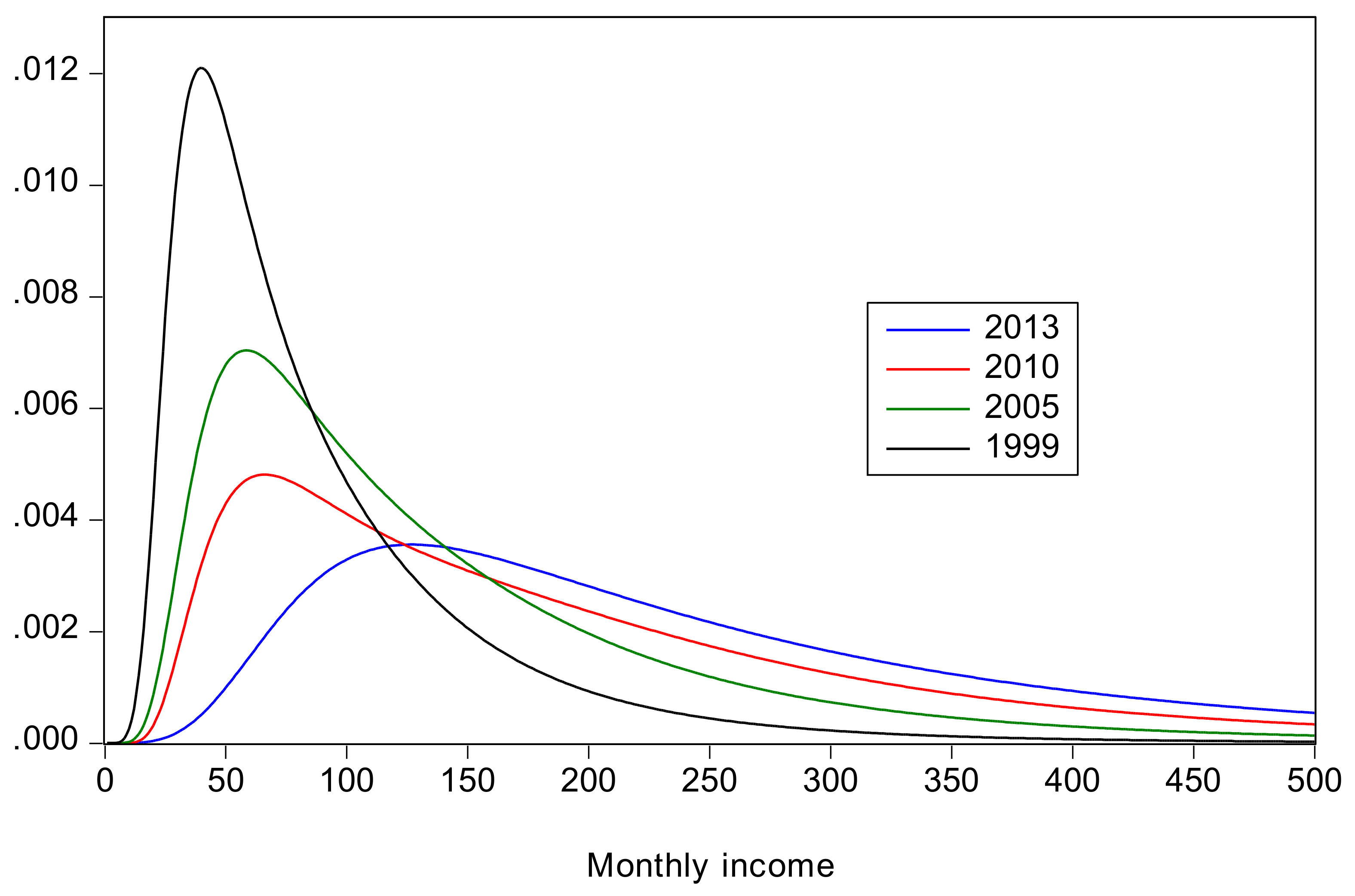
• All inequality measures indicate that inequality increased from 1999 to 2010, and then declined from 2010 to 2013. The recent decline is attributable to a decline in rural inequality; there was an increase in urban inequality in the same period. Also, there is no clear conclusion about how rural inequality changed from 1999 to 2005; the Gini and $I(1)$ suggest a slight decrease, whereas QSR, $I(0)$ and Pietra suggest a slight increase.
• Inequality is much greater in the combined distribution than in its components, reflecting the large discrepancy in mean incomes between the rural and urban areas. Within inequality remains greater than between inequality, however.
• The changes in inequality have been accompanied by large increases in mean income and large decreases in poverty. The decline in poverty was particularly dramatic for rural China where the headcount ratio declined from 57% in 1999 to 3.7% in 2013. Poverty in rural China is uniformly greater than that in urban China.
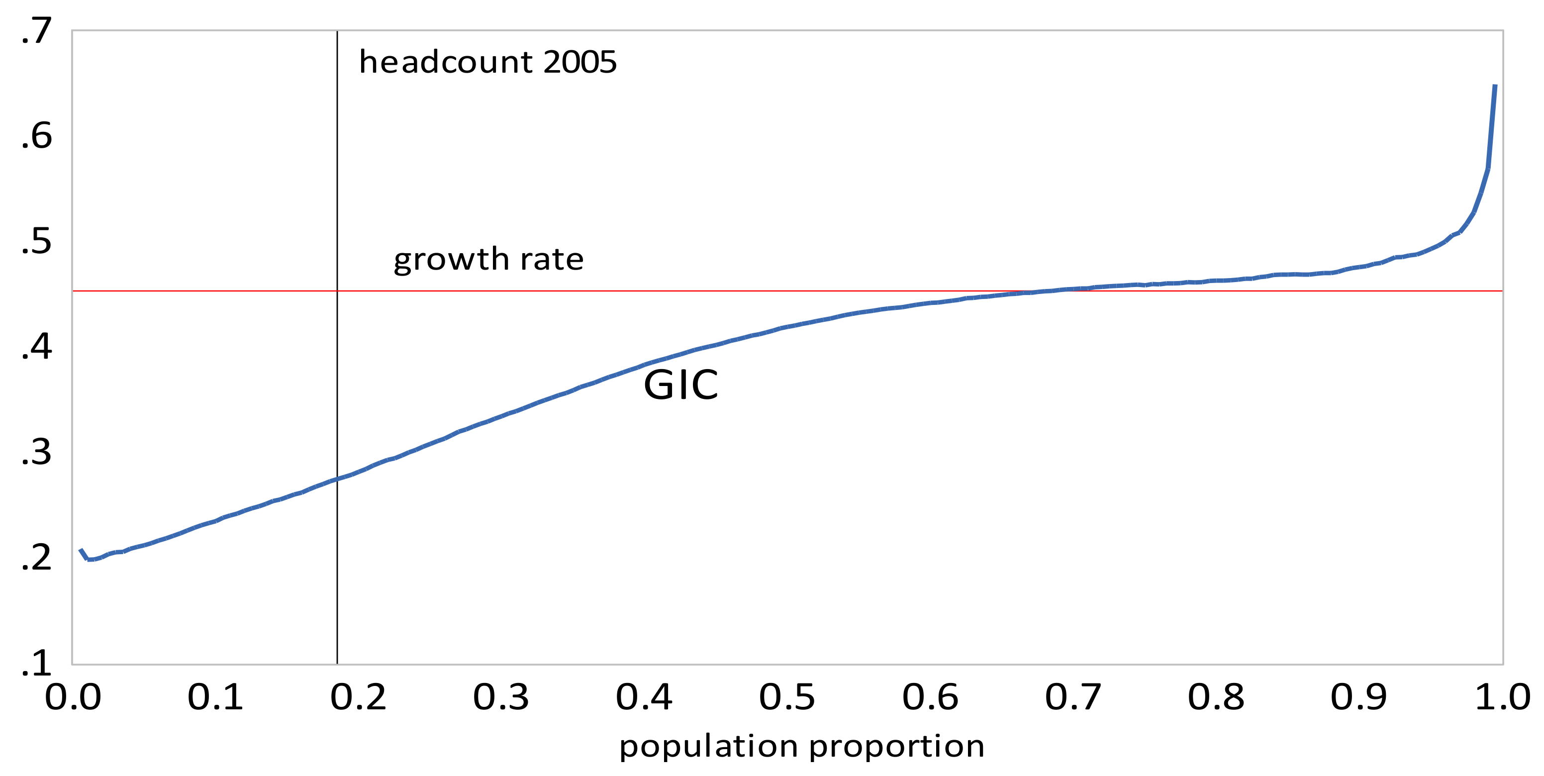
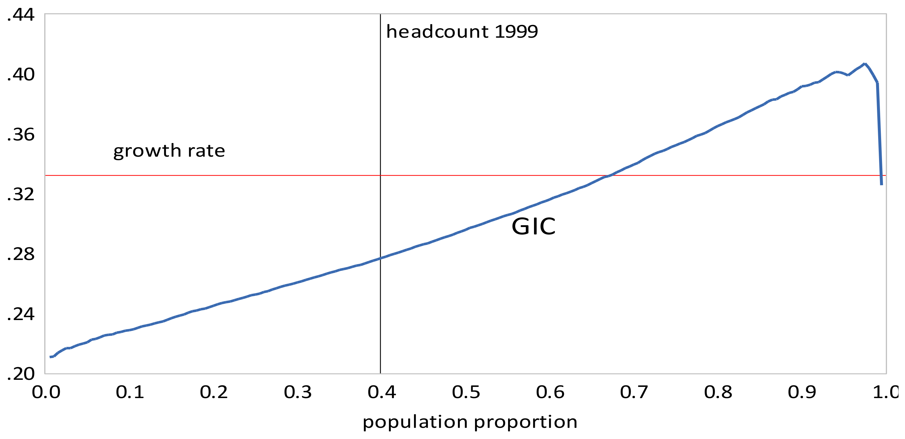
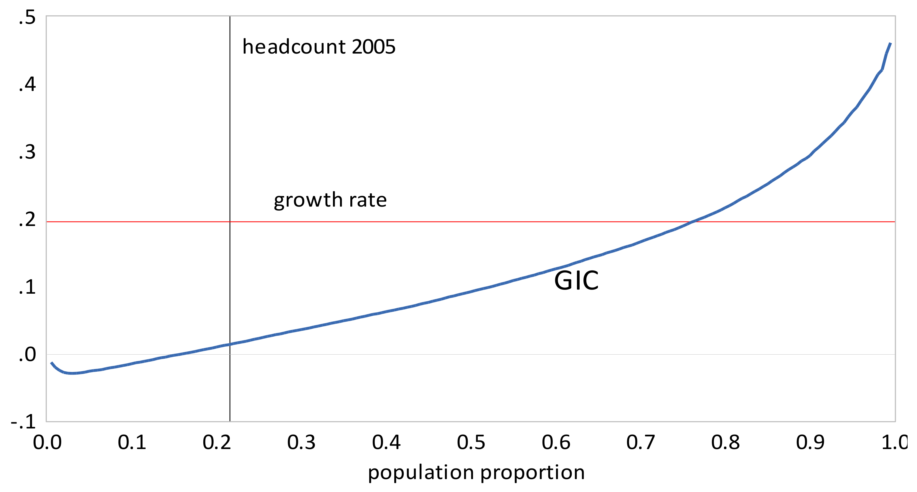
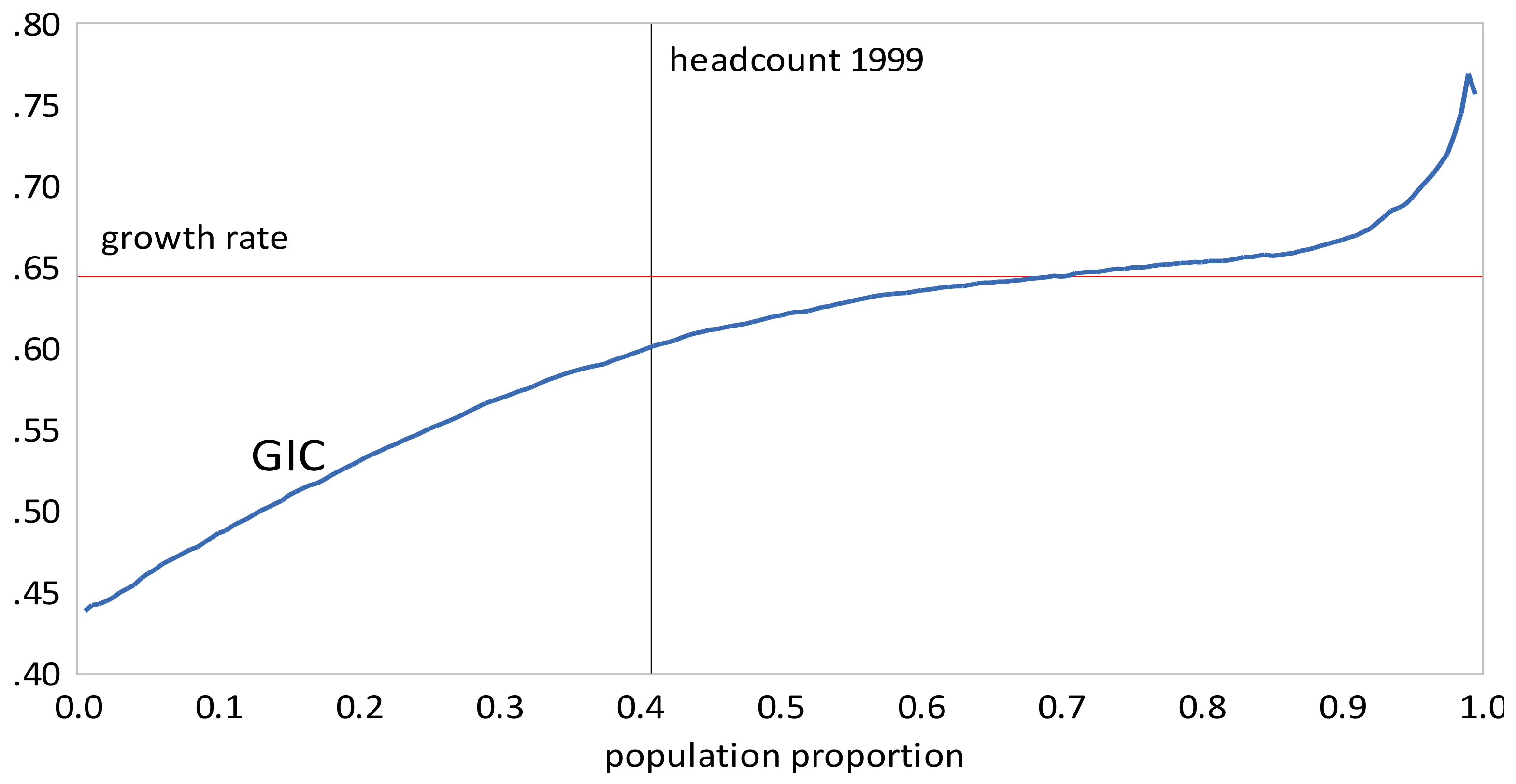
• The GIC curves show that, from 1999 to 2010, growth has favored the rich more than the poor, but from 2010 to 2013, growth has strongly favored the poor relative to the rich, a result consistent with the decline in inequality over this period. The scalar measures of pro-poor growth are also consistent with this observation. Growth has favured the poor in an absolute sense from 1999 to 2010 $(0<RC<g$, $0<KP<1$, $PEGR<g)$, and in a relative sense after 2010 $(RC>g$, $KP>1$, $PEGR>g)$.

Examining the results for Indonesia, we find:

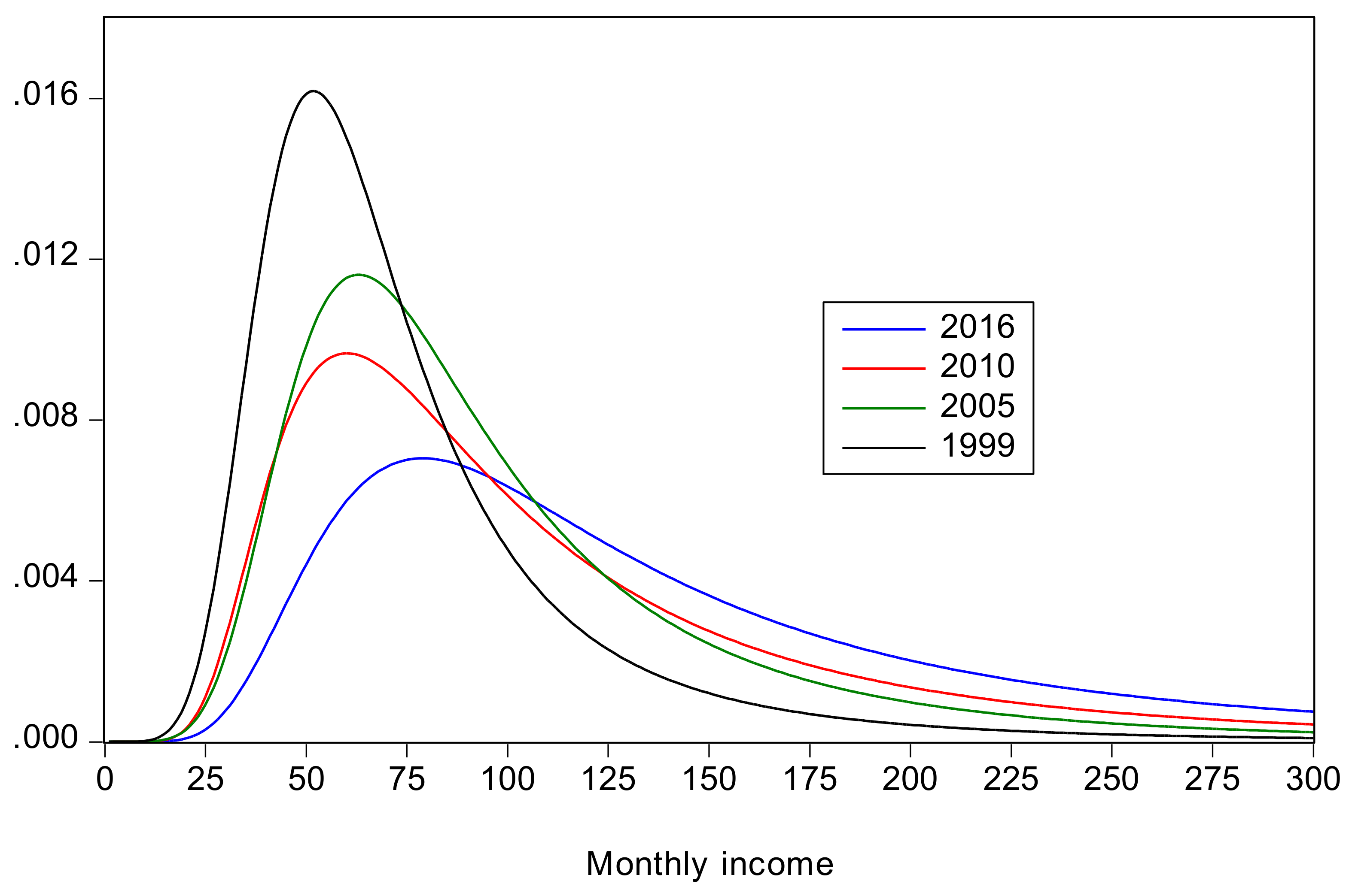
• Urban inequality changed very little from 1999 to 2005, increased dramatically from 2005 to 2010, and then increased more moderately from 2010 to 2016. Rural inequality increased from 1999 to 2010, but declined thereafter. The combined results reflect these changes, with increasing inequality overall, but with Gini coefficients approximately the same in 2010 and 2016.
• Poverty declined from 1999 to 2005, remained roughly constant from 2005 to 2010, when there were large increases in inequality, and then declined again from 2010 to 2016. From 2005 to 2010 a decline in urban poverty was offset by an increase in rural poverty.
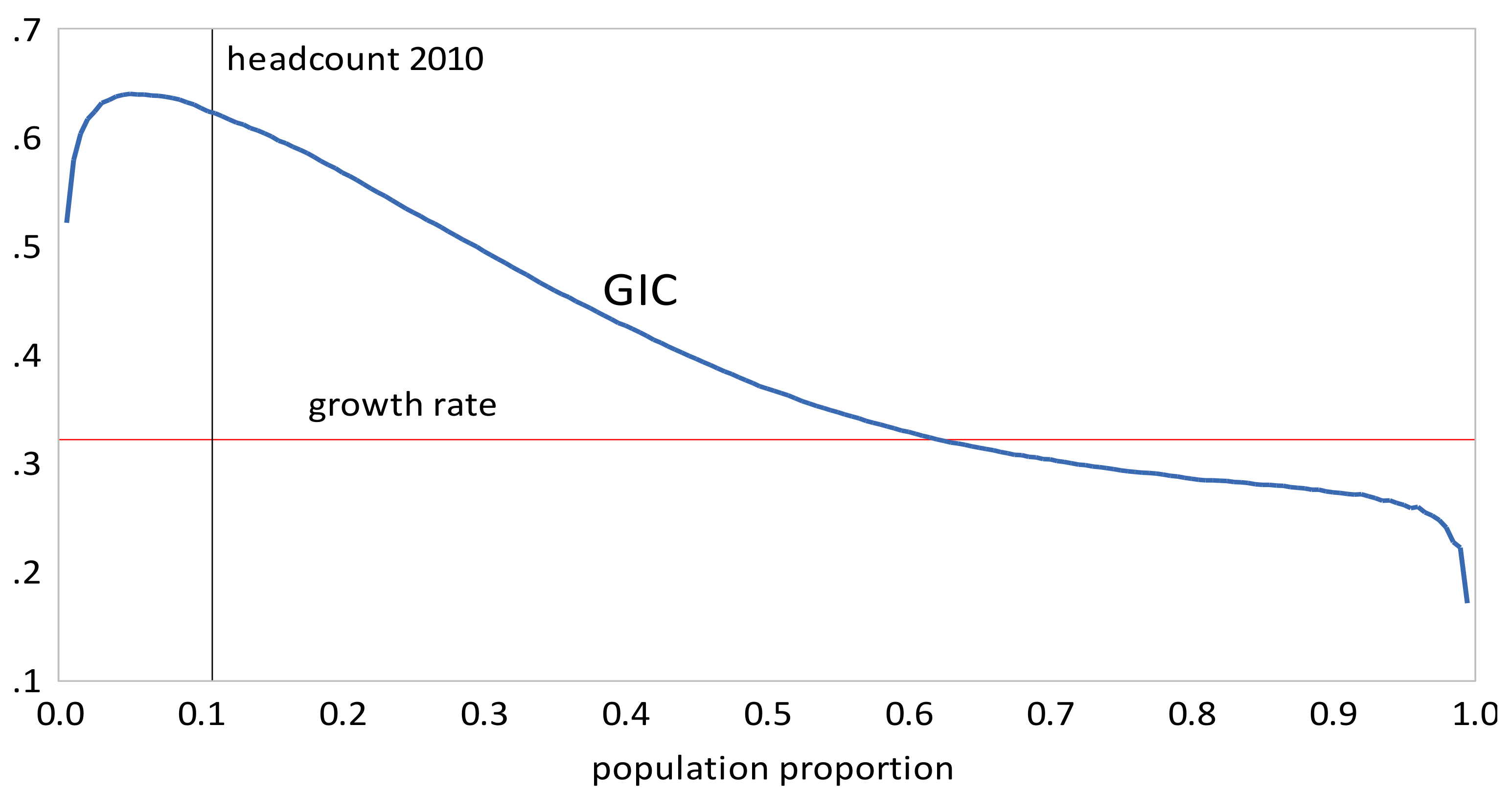
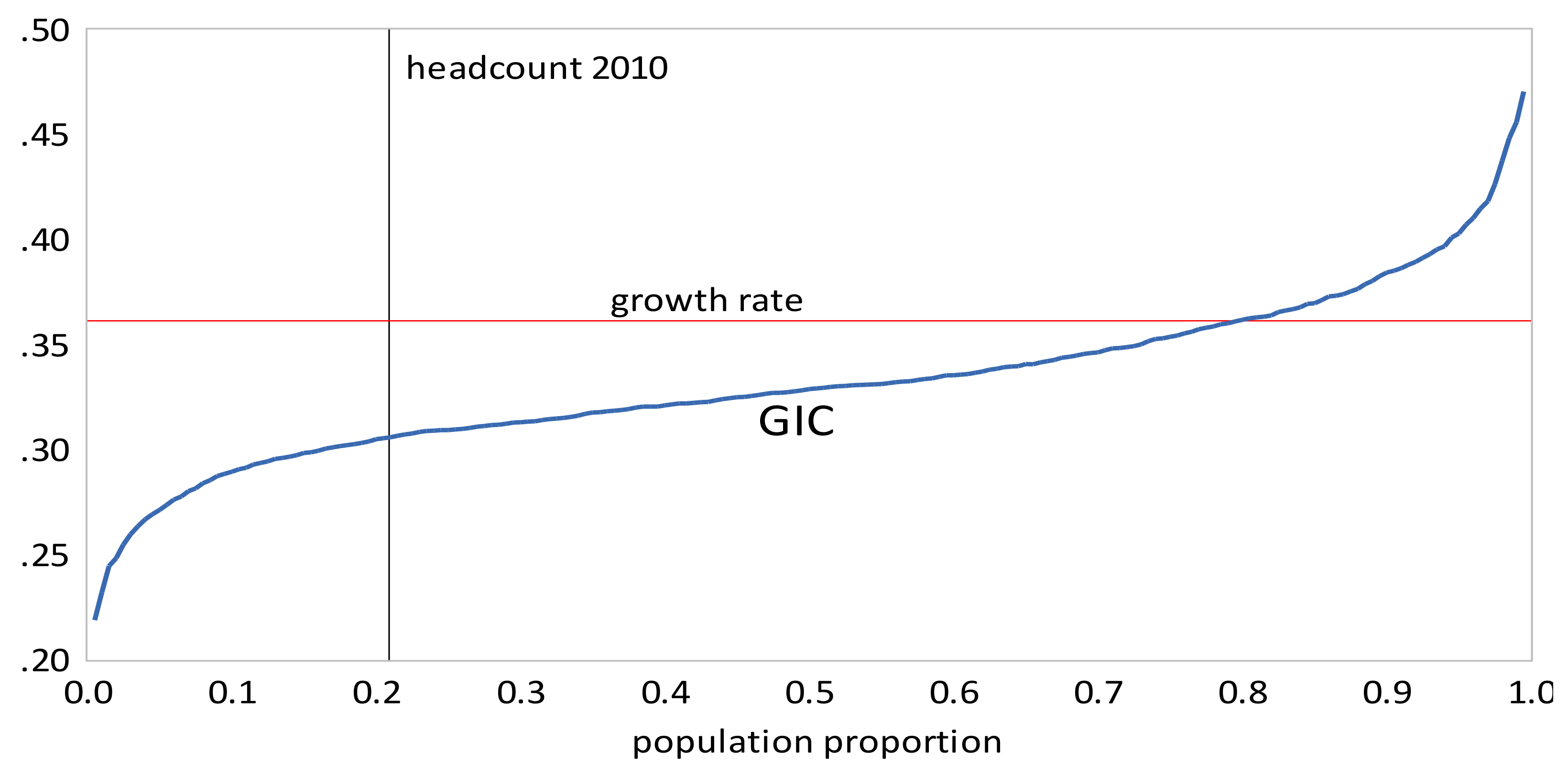
• The GIC curves show that growth has favored the rich relative to the poor in all time intervals. From 2005 to 2010 the poor faired very badly; the growth rate for the bottom 15% of the population was negative. This period was also one where the growth in mean incomes was low relative to that in the other two periods. The scalar pro-poor growth measures are in line with the conclusions from the GIC curves. Growth was absolutely but not relatively pro-poor in the first and third time intervals; in the second interval it was not absolutely pro-poor according to the RC measure, and only slightly absolutely pro-poor using the KP measure.

5. Concluding Remarks

Studying income distributions can provide valuable information about important aspects of a society’s welfare such as the degree of inequality, the incidence of poverty, and whether there have been improvements in welfare over time. The GB2 is a popular and versatile distribution well suited to this purpose. We have reviewed some of the common indexes for measuring inequality, poverty and pro-poor growth, and described how values for these indexes can be computed from estimates of the parameters of the GB2 distribution. Optimal techniques for estimating the parameters using either single observations or grouped data are also reviewed. It is our hope that the bringing together of all these results into a single source will facilitate and promote use of the GB2 distribution.

References

- Biewen, Martin, and Stephen P. Jenkins. 2005. A Framework for the Decomposition of Poverty Differences with an Application to Poverty Differences between Countries. Empirical Economics 30: 331–58. [Google Scholar] [CrossRef]
- Bordley, Robert F., James B. McDonald, and Anand Mantrala. 1997. Something New, Something Old: Parametric Models for the Size of Distribution of Income. Journal of Income Distribution 6: 91–103. [Google Scholar]
- Butler, Richard J., and James B. McDonald. 1986. Income Inequality in the U.S.: 1948–80. Research in Labor Economics 8: 85–140. [Google Scholar]
- Butler, Richard J., and James B. McDonald. 1989. Using Incomplete Moments to Measure Inequality. Journal of Econometrics 42: 109–20. [Google Scholar] [CrossRef]
- Chotikapanich, Duangkamon, ed. 2008. Modeling Income Distributions and Lorenz Curves. New York: Springer. [Google Scholar]
- Chotikapanich, Duangkamon, William Griffiths, Wasana Karunarathne, and D. S. Prasada Rao. 2013. Calculating Poverty Measures from the Generalized Beta Income Distribution. Economic Record 89: 48–66. [Google Scholar] [CrossRef]
- Chotikapanich, Duangkamon, William E. Griffiths, and D. S. Prasada Rao. 2007. Estimating and Combining National Income Distributions Using Limited Data. Journal of Business and Economic Statistics 25: 97–109. [Google Scholar] [CrossRef]
- Chotikapanich, Duangkamon, William E. Griffiths, D. S. Prasada Rao, and Vicar Valencia. 2012. Global Income Distributions and Inequality, 1993 and 2000: Incorporating Country-level Inequality Modeled with Beta Distributions. The Review of Economics and Statistics 94: 52–73. [Google Scholar] [CrossRef]
- Cummins, John, Georges Dionne, James McDonald, and B. Michael Pritchett. 1990. Applications of the GB2 Family of Distributions in Modeling Insurance Loss Processes. Insurance: Mathematics and Economics 9: 257–72. [Google Scholar] [CrossRef]
- Duclos, Jean-Yves, and Audrey Verdier-Chouchane. 2010. Analyzing Pro-Poor Growth in Southern Africa: Lessons from Mauritius and South Africa. Working Papers Series No. 115. Tunis: African Development Bank. [Google Scholar]
- Feng, Shuaizhang, Richard Burkhauser, and J. S. Butler. 2006. Levels and Long-Term Trends in Earnings Inequality: Overcoming Current Population Survey Censoring Problems Using the GB2 Distribution. Journal of Business and Economic Statistics 24: 57–62. [Google Scholar] [CrossRef]
- Foster, James, Joel Greer, and Erik Thorbecke. 1984. A Class of Decomposable Poverty Measures. Econometrica 52: 761–66. [Google Scholar] [CrossRef]
- Graf, Monique. 2009. An Efficient Algorithm for the Computation of the Gini Coefficient of the Generalised Beta Distribution of the Second Kind. In JSM Proceedings, Business and Economic Statistics Section. Alexandria: American Statistical Association, pp. 4835–43. [Google Scholar]
- Graf, Monique, and Desislava Nedyalkova. 2014. Modeling of Income and Indicators of Poverty and Social Exclusion Using the Generalized Beta Distribution of the Second Kind. Review of Income and Wealth 60: 821–42. [Google Scholar] [CrossRef]
- Greene, William H. 2012. Econometric Analysis, 7th ed. New York: Prentice Hall. [Google Scholar]
- Griffiths, William, and Gholamreza Hajargasht. 2015. On GMM Estimation of Distributions from Grouped Data. Economics Letters 126: 122–26. [Google Scholar] [CrossRef]
- Hajargasht, Gholamreza, and William E. Griffiths. 2013. Pareto-Lognormal Distributions: Inequality, Poverty, and Estimation from Grouped Income Data. Economic Modelling 33: 593–604. [Google Scholar] [CrossRef]
- Hajargasht, Gholamreza, William E. Griffiths, Joseph Brice, D. S. Prasada Rao, and Duangkamon Chotikapanich. 2012. Inference for Income Distributions Using Grouped Data. Journal of Business of Economic Statistics 30: 563–76. [Google Scholar] [CrossRef]
- Jenkins, Stephen P. 2009. Distributionally-Sensitive Inequality Indices and the GB2 Income Distribution. Review of Income and Wealth 55: 392–98. [Google Scholar] [CrossRef]
- Jones, Andrew M., James Lomas, and Nigel Rice. 2014. Applying Beta-Type Size Distributions to Healthcare Cost Regressions. Journal of Applied Econometrics 29: 649–70. [Google Scholar] [CrossRef]
- Kakwani, Nanak, and Ernesto M. Pernia. 2000. What is Pro-Poor Growth. Asian Development Review 18: 1–16. [Google Scholar]
- Kakwani, Nanak, Shahidur R. Khandker, and Hyun Son. 2004. Pro-Poor Growth: Concepts and Measurement with Country Case Studies. Working Paper No. 1. Brasilia: International Poverty Centre, United Nations Development Programme. [Google Scholar]
- Kleiber, Christian, and Samuel Kotz. 2003. Statistical Size Distributions in Economics and Actuarial Sciences. New York: John Wiley and Sons. [Google Scholar]
- McDonald, James B. 1984. Some Generalized Functions for the Size Distribution of Income. Econometrica 52: 647–63. [Google Scholar] [CrossRef]
- McDonald, James B., and Michael Ransom. 2008. The Generalized Beta Distribution as a Model for the Distribution of Income: Estimation of Related Measures of Inequality. In Modeling Income Distributions and Lorenz Curves. Edited by Duangkamon Chotikapanich. New York: Springer, pp. 147–66. [Google Scholar]
- McDonald, James B., Jeff Sorensen, and Patrick A. Turley. 2011. Skewness and Kurtosis Properties of Income Distribution Models. Review of Income and Wealth 59: 360–74. [Google Scholar] [CrossRef]
- McDonald, James B., and Yexiao J. Xu. 1995. A generalization of the beta distribution with applications. Journal of Econometrics 66: 133–52, Erratum in Journal of Econometrics 69: 427–28. [Google Scholar] [CrossRef]
- Parker, Simon C. 1999. The Generalized Beta as a Model for the Distribution of Earnings. Economics Letters 62: 197–200. [Google Scholar] [CrossRef]
- Quintano, Claudio, and Antonella D’Agostino. 2006. Studying Inequality in Income Distribution of Single-Person Households in Four Developed Countries. Review of Income and Wealth 52: 525–46. [Google Scholar] [CrossRef]
- Ravallion, Martin, and Shaohua Chen. 2003. Measuring Pro-Poor Growth. Economics Letters 78: 93–99. [Google Scholar] [CrossRef]
- Sarabia, José María, and Vanesa Jordá. 2014. Explicit Expressions of the Pietra Index for the Generalized Function for the Size Distribution of Income. Physica A 416: 582–89. [Google Scholar] [CrossRef]
- Sarabia, José María, Vanesa Jordá, and Lorena Remuzgo. 2017. The Theil Indices in Parametric Families of Income Distributions—A Short Review. Review of Income and Wealth 63: 867–80. [Google Scholar] [CrossRef]
- Sen, Amartya K. 1976. Poverty: An Ordinal Approach to Measurement. Econometrica 44: 219–31. [Google Scholar] [CrossRef]
- Theil, Henri. 1967. Economics and Information Theory. Amsterdam: North Holland. [Google Scholar]
- Watts, Harold W. 1968. An Economic Definition of Poverty. In On Understanding Poverty. Edited by Daniel P. Moyniham. New York: Basic Books, pp. 316–29. [Google Scholar]