Copula–Based vMEM Specifications versus Alternatives: The Case of Trading Activity

Abstract

We discuss several multivariate extensions of the Multiplicative Error Model to take into account dynamic interdependence and contemporaneously correlated innovations (vector MEM or vMEM). We suggest copula functions to link Gamma marginals of the innovations, in a specification where past values and conditional expectations of the variables can be simultaneously estimated. Results with realized volatility, volumes and number of trades of the JNJ stock show that significantly superior realized volatility forecasts are delivered with a fully interdependent vMEM relative to a single equation. Alternatives involving log–Normal or semiparametric formulations produce substantially equivalent results.

1. Introduction

Dynamics in financial markets can be characterized by many indicators of trading activity such as absolute returns, high-low range, number of trades in a certain interval (possibly labeled as buys or sells), volume, ultra-high frequency based measures of volatility, financial durations, spreads and so on.

Engle (2002) reckons that one striking regularity behind financial time series is that persistence and clustering characterizes the evolution of such processes. As a result, the dynamics of such variables can be specified as the product of a conditionally deterministic scale factor, which evolves according to a GARCH–type equation, and an innovation term which is iid with unit mean. Such models are labeled Multiplicative Error Models (MEM) and can be seen as a generalization of the GARCH (Bollerslev 1986) and of the Autoregressive Conditional Duration (ACD, Engle and Russell (1998)) approaches. One of the advantages of such a model is to avoid the need to resort to logs (not possible when zeros are present in the data) and to provide conditional expectations of the variables of interest directly (rather than expectations of the logs). Empirical results show a good performance of these types of models in capturing the stylized facts of the observed series (e.g., for daily range, Chou (2005); for volatility, volume and trading intensity Hautsch (2008)).

The model was specified by Engle and Gallo (2006) in a multivariate context (vector MEM or vMEM) allowing just the lagged values of each variable of interest to affect the conditional expectation of the other variables. Such a specification lends itself to producing multi–step ahead forecasts: in Engle and Gallo (2006) three different measures of volatility (absolute returns, daily range and realized volatility), influence each other dynamically. Although such an equation–by–equation estimation ensures consistency of the estimators in a quasi-maximum likelihood context, given the stationarity conditions discussed by Engle (2002), correlation among the innovation terms is not taken into account and leads to a loss in efficiency.

However, full interdependence is not allowed by an equation–by–equation approach both in the form of past conditional expectations influencing the present and a contemporaneous correlations of the innovations. The specification of a multivariate distribution of the innovations is far from trivial: a straightforward extension to a joint Gamma probability distribution is not available except in very special cases. In this paper, we want to compare the features of a novel maximum likelihood estimation strategy adopting copula functions to other parametric and semiparametric alternatives. Copula functions allow to link together marginal probability density functions for individual innovations specified as Gamma as in Engle and Gallo (2006) or as zero–augmented distributions (as in Hautsch et al. (2013), distinguishing between the zero occurrences and the strictly positive realizations). Copula functions are used in a Multiplicative Error framework, but in a Dynamic Conditional Correlation context by Bodnar and Hautsch (2016). Within a Maximum Likelihood approach to the vector MEM, we want also to explore the performance of a multivariate log–Normal specification for the joint distribution of the innovations and the semiparametric approach presented in Cipollini et al. (2013) resulting in a GMM estimator. The range of potential applications of a vector MEM is quite wide: dynamic interactions among different values of volatility, volatility spillovers across markets (allowing multivariate-multi-step ahead forecasts and impulse response functions, order execution dynamics Noss (2007) specifies a MEM for execution depths).

This paper aims at discussing merits of each approach and their performance in forecasting realized volatility with augmented information derived from the dynamic interaction with other measures of market activity (namely, the volumes and the number of trades). We want conditional expectations to depend just on past values (not also on some contemporary information as in Manganelli (2005) and Hautsch (2008)).

What the reader should expect is the following: in Section 2 we lay out the specification of a vector Multiplicative Error Model, discussing the issues arising from the adoption of several types of copula functions linking univariate Gamma marginal distributions. In Section 3 we describe the Maximum Likelihood procedure leading to the inference on the parameters. In Section 4 we discuss the features of a parametric specification with a log–Normal and of a semiparametric approach suggested by Cipollini et al. (2013). In Section 5 we present the empirical application to three series of market trading activity, namely realized kernel volatility, traded volumes and the number of trades. The illustration is performed on the JNJ stock over a period between 2007 and 2013. What we find is that specifying the joint distribution of the innovations allowing for contemporaneous correlation dramatically improves the log–likelihood over an independent (i.e., equation–by–equation) approach. Richer specifications (where simultaneous estimation is unavoidable) deliver a better fit, improved serial correlation diagnostics, and a better performance in out–of–sample forecasting. The Student–T copula possesses better features than the Normal copula. Overall, the indication is that we will have significantly superior realized volatility forecasts when other trading activity indicators and contemporaneous correlations are considered. Concluding remarks follow.

2. A Copula Approach to Multiplicative Error Models

Let ${\mathit{x}}_t$ be a K–dimensional process with non–negative components. A vector Multiplicative Error Model (vMEM) for ${\mathit{x}}_t$ is defined as

$${\mathit{x}}_t={\mathit{\mu }}_t\odot {\mathit{\epsilon }}_t=diag({\mathit{\mu }}_t){\mathit{\epsilon }}_t,$$

(1)

where ⊙ indicates the Hadamard (element–by–element) product and $diag(·)$ indicates a diagonal matrix with its vector argument on the main diagonal. Conditionally upon the information set ${\mathcal{F}}_{t-1}$, a fairly general specification for ${\mathit{\mu }}_t$ is

$${\mathit{\mu }}_t=\mathit{\omega }+\mathit{\alpha }{\mathit{x}}_{t-1}+\mathit{\gamma }{\mathit{x}}_{t-1}^{(-)}+\mathit{\beta }{\mathit{\mu }}_{t-1},$$

(2)

where $\mathit{\omega }$ is $(K,1)$ and $\mathit{\alpha }$, $\mathit{\gamma }$ and $\mathit{\beta }$ are $(K,K)$. The vector ${\mathit{x}}_t^{(-)}$ has a generic element $x_{t,i}$ multiplied by a function related to a signed variable, be it a positive or negative return ($0,1$ values) or a signed trade (buy or sell $1,-1$ values), as to capture asymmetric effects. Let the parameters relevant for ${\mathit{\mu }}_t$ be collected in a vector $\mathit{\theta }$.

Conditions for stationarity of ${\mathit{\mu }}_t$ are a simple generalization of those of the univariate case (e.g., Bollerslev (1986); Hamilton (1994)): a vMEM(1,1) with ${\mathit{\mu }}_t$ defined as in Equation (2) is stationary in mean if all characteristic roots of $\mathit{A}=\mathit{\alpha }+\mathit{\beta }+\mathit{\gamma }/2$ are smaller than 1 in modulus. We can think of $\mathit{A}$ as the impact matrix in the expression

$$E\left({\mathit{x}}_{t+1}|{\mathcal{F}}_{t-1}\right)={\mathit{\mu }}_{t+1|t-1}=\mathit{\omega }+\mathit{A}{\mathit{\mu }}_{t|t-1}.$$

If more lags are considered, the model is

$${\mathit{\mu }}_t=\mathit{\omega }+\sum _{l=1}^L\left[{\mathit{\alpha }}_l{\mathit{x}}_{t-l}+{\mathit{\gamma }}_l{\mathit{x}}_{t-l}^{(-)}+{\mathit{\beta }}_l{\mathit{\mu }}_{t-l}\right],$$

(3)

where L is the maximum lag occurring in the dynamics. It is often convenient to represent the system (3) in its equivalent companion form

$${\mathit{\mu }}_{t+L|t-1}^{*}=\mathit{\omega }+{\mathit{A}}^{*}{\mathit{\mu }}_{t+L-1|t-1}^{*},$$

(4)

where ${\mathit{\mu }}_{t+L|t-1}^{*}=({\mathit{\mu }}_{t+L|t-1};{\mathit{\mu }}_{t+L-1|t-1};\dots ;{\mathit{\mu }}_{t+1|t-1})$ is a $KL\times 1$ vector obtained by stacking its elements columnwise and

$${\mathit{A}}^{*}=\left(\begin{array}{cccc}{\mathit{A}}_1& {\mathit{A}}_2& \cdots & {\mathit{A}}_L\\ & {\mathit{I}}_{K(L-1)}& & {\mathbf{0}}_{K(L-1),K}\end{array}\right)$$

with ${\mathit{A}}_l={\mathit{\alpha }}_l+{\mathit{\beta }}_l+{\mathit{\gamma }}_l/2,l=1,\dots ,L$, ${\mathit{I}}_{K(L-1)}$ is a $K(L-1)\times K(L-1)$ identity matrix and ${\mathbf{0}}_{K(L-1),K}$ is a $K(L-1)\times K$ matrix of zeros. The same stationarity condition holds in terms of eigenvalues of ${\mathit{A}}^{*}$.

The innovation vector ${\mathit{\epsilon }}_t$ is a K–dimensional iid process with probability density function (pdf) defined over a ${[0,+\infty )}^K$ support, the unit vector $𝕝$ as expectation and a general variance–covariance matrix $\mathsf{\Sigma }$,

$${\mathit{\epsilon }}_t|{\mathcal{F}}_{t-1}\sim D^{+}(𝕝,\mathsf{\Sigma }).$$

(5)

The previous conditions guarantee that

$$\begin{array}{cc}\hfill E({\mathit{x}}_t|{\mathcal{F}}_{t-1})& ={\mathit{\mu }}_t\hfill \end{array}$$

(6)

$$\begin{array}{cc}\hfill V({\mathit{x}}_t|{\mathcal{F}}_{t-1})& ={\mathit{\mu }}_t{\mathit{\mu }}_t^{\prime }\odot \mathsf{\Sigma }=diag({\mathit{\mu }}_t)\mathsf{\Sigma }diag({\mathit{\mu }}_t),\hfill \end{array}$$

(7)

where the latter is a positive definite matrix by construction.

The distribution of the error term ${\mathit{\epsilon }}_t|{\mathcal{F}}_{t-1}$ can be specified in different ways. We discuss here a flexible approach using copula functions; different specifications are presented in Section 4.

Using copulas (cf., among others, Joe (1997) and Nelsen (1999), Embrechts et al. (2002), Cherubini et al. (2004), McNeil et al. (2005) and the review of Patton (2013) for financial applications), the conditional pdf of ${\mathit{\epsilon }}_t|{\mathcal{F}}_{t-1}$ is given by

$$f_{\mathit{\epsilon }}\left({\mathit{\epsilon }}_t|{\mathcal{F}}_{t-1}\right)=c\left({\mathit{u}}_t;\mathit{\xi }\right)\prod _{i=1}^K{f}_i\left({\epsilon }_{t,i};{\mathit{\varphi }}_i\right),$$

(8)

where $c({\mathit{u}}_t;\mathit{\xi })$ is the pdf of the copula, $f_i({\epsilon }_{t,i};{\mathit{\varphi }}_i)$ and $u_{t,i}=F_i({\epsilon }_{t,i};{\mathit{\varphi }}_i)$ are the pdf and the cdf, respectively, of the marginals, $\mathit{\xi }$ and ${\mathit{\varphi }}_i$ are parameters. A copula approach, hence, requires the specification of two objects: the distribution of the marginals and the copula function.

In view of the flexible properties shown elsewhere (Engle and Gallo 2006), for the first we adopt Gamma pdf’s (but other choices are possible, such as Inverse-Gamma, Weibull, log–Normal, and mixtures of them). This has the important feature of guaranteeing an interpretation of a Quasi Maximum Likelihood Estimator even if the choice of the distribution is not appropriate. For the second, we discuss some possible specifications within the class of Elliptical copulas which provides an unified framework encompassing the Normal, the Student-T and any other member of this family endowed with an explicit pdf.

Elliptical copulas have interesting features and widespread applicability in Finance (for details see McNeil et al. (2005), Frahm et al. (2003), Schmidt (2002)). They are copulas generated by Elliptical distributions, exactly in the same way as the Normal copula and the Student-T copula stem from the multivariate Normal and Student-T distributions, respectively.1

We consider a copula generated by an Elliptical distribution whose univariate ‘standardized’ marginals (intended here with location parameter 0 and dispersion parameter 1) have an absolutely continuous symmetric distribution, centered at zero, with pdf $g(.;\mathit{\nu })$ and cdf $G(.;\mathit{\nu })$ ($\mathit{\nu }$ represents a vector of shape parameters). The density of the copula can then be written as

$${\displaystyle c_E\left(\mathit{u};\mathit{R},\mathit{\nu }\right)=K^{*}\left(\mathit{\nu },K\right){|\mathit{R}|}^{-1/2}\frac{g_1\left({\mathit{q}}^{\prime }{\mathit{R}}^{-1}\mathit{q};\mathit{\nu },K\right)}{{\prod }_{i=1}^K{g}_2\left(q_i^2;\mathit{\nu }\right)}}$$

(9)

for suitable choices of $K^{*}(.,.)$, $g_1(.;.,.)$ and $g_2(.;.)$, where $\mathit{q}=(q_1;\dots ;q_K)$, $q_i=G^{-1}(u_i;\mathit{\nu })$.

Two notable cases will be considered. The first is the Normal copula (McNeil et al. (2005), Cherubini et al. (2004), Bouyé et al. (2000)); with no explicit shape parameter $\mathit{\nu }$, we have $K^{*}(K)\equiv 1$, $g_1(x;K)=g_2(x)\equiv exp(-x/2)$. The pdf in Equation (9) becomes:

$$c_N(\mathit{u};\mathit{R})={|\mathit{R}|}^{-1/2}exp\left[-\frac{1}{2}\left({\mathit{q}}^{\prime }{\mathit{R}}^{-1}\mathit{q}-{\mathit{q}}^{\prime }\mathit{q}\right)\right],$$

(10)

where $\mathit{q}=(q_1;\dots ;q_K)$, $q_i={\mathsf{\Phi }}^{-1}(u_i)$ and $\mathsf{\Phi }(x)$ denotes the cdf of the standard Normal distribution computed at x.

The Normal copula has many interesting properties: the ability to reproduce a broad range of dependencies (the bivariate version, according to the value of the correlation parameter, is capable of attaining the lower Fréchet bound, the product copula and the upper Fréchet bound), the analytical tractability, the ease of simulation. When combined with $Gamma({\varphi }_i,{\varphi }_i)$ marginals, the resulting multivariate distribution is a special case of dispersion distribution generated from a Gaussian copula (Song 2000). We note that the conditional correlation matrix of ${\mathit{\epsilon }}_t$ has generic element approximately equal to $R_{ij}$, which can assume negative values too.

One of the limitations of the Normal copula is the asymptotic independence of its tails. Empirically, tail dependence is a behavior observed frequently in financial time series (see McNeil et al. (2005), among others). Elements of $\mathit{x}$ (being different indicators of the same asset or different assets) tend to be affected by the same extreme events. For this reason, as an alternative, we consider the Student-T copula which allows for asymptotically dependent tails. Differently from the Normal copula, when $\mathit{R}=\mathit{I}$ we get uncorrelated but not independent marginals (details in McNeil et al. (2005)). Thus, when considering the Student-T copula in Equation (9), with a scalar $\nu$ shape parameter, we have ${\displaystyle K^{*}(\nu ;K)=\frac{\mathsf{\Gamma }((\nu +K)/2)\mathsf{\Gamma }{(\nu /2)}^{K-1}}{\mathsf{\Gamma }((\nu +1)/2)}}$, $g_1(x;\nu ,K)={(1+x/\nu )}^{-(\nu +K)/2}$, $g_2(x;\nu )={(1+x/\nu )}^{-(\nu +1)/2}$, and its explicit pdf is

$$c_T\left(\mathit{u};\mathit{R},\nu \right)=\frac{\mathsf{\Gamma }(\left(\nu +K\right)/2)\mathsf{\Gamma }{\left(\nu /2\right)}^{K-1}}{\mathsf{\Gamma }((\nu +1)/2)}{|\mathit{R}|}^{-1/2}\frac{(1+{\mathit{q}}^{\prime }{\mathit{R}}^{-1}\mathit{q}{/\nu )}^{-(\nu +K)/2}}{{\prod }_{i=1}^K(1+{q_i^2/\nu )}^{-(\nu +1)/2}},$$

(11)

where $\mathit{q}=(q_1;\dots ;q_K)$, $q_i=T^{-1}(u_i;\nu )$ and $T(x;\nu )$ denotes the cdf of the Student-T distribution with $\nu$ degrees of freedom computed at x. Further specifications of the Student-T copula are in Demarta and McNeil (2005).

3. Maximum Likelihood Inference

In this section we discuss how to get full Maximum Likelihood (ML) inferences from the vMEM with the parametric specification (3) for ${\mathit{\mu }}_t$ (dependent on a parameter vector $\mathit{\theta }$) and a copula-based formulation $f_{\mathit{\epsilon }}({\mathit{\epsilon }}_t|{\mathcal{F}}_{t-1})$ of the conditional distribution of the vector error term (characterized by the parameter vector $\mathit{\lambda }$). Inference on $\mathit{\theta }$ and $\mathit{\lambda }$ can be discussed in turn, given that from the model assumptions the log-likelihood function l is

$$\begin{array}{ccc}\hfill l& =& \sum _{t=1}^{T}ln{f}_{\mathit{x}}\left({\mathit{x}}_t|{\mathcal{F}}_{t-1}\right)=\sum _{t=1}^{T}ln\left(f_{\mathit{\epsilon }}\left({\mathit{\epsilon }}_t|{\mathcal{F}}_{t-1}\right)\prod _{i=1}^K{\mu }_{t,i}^{-1}\right)\hfill \\ & =& \sum _{t=1}^T\left[ln{f}_{\mathit{\epsilon }}\left({\mathit{\epsilon }}_t|{\mathcal{F}}_{t-1}\right)-\sum _{i=1}^{K}ln{\mu }_{t,i}\right].\hfill \end{array}$$

(12)

Considering a generic time t, it is useful to recall the sequence of calculations:

$${\mu }_{t,i}({\mathit{\theta }}_i)\to x_{t,i}/{\mu }_{t,i}={\epsilon }_{t,i}\to F_i({\epsilon }_{t,i};{\mathit{\varphi }}_i)=u_{t,i}\to c({\mathit{u}}_t;\mathit{\xi })i=1,\dots ,K$$

(13)

where ${\mathit{\theta }}_i$ is the parameter involved in the i-th element of the ${\mathit{\mu }}_t$ vector.

3.1. Parameters in the Conditional Mean

Irrespective of the specification chosen for $f_{\mathit{\epsilon }}({\mathit{\epsilon }}_t|{\mathcal{F}}_{t-1})$, the structure of the vMEM allows to express the portion of the score function corresponding to $\mathit{\theta }$ as

$${\nabla }_{\mathit{\theta }}l=-\sum _{t=1}^T{\mathit{A}}_t{\mathit{w}}_t$$

(14)

where

$${\mathit{A}}_t={\nabla }_{\mathit{\theta }}{\mathit{\mu }}_t^{\prime }diag{({\mathit{\mu }}_t)}^{-1},$$

(15)

$${\mathit{w}}_t={\mathit{\epsilon }}_t\odot {\mathit{b}}_t+𝕝,$$

(16)

$${\mathit{b}}_t={\nabla }_{{\mathit{\epsilon }}_t}lnf\left({\mathit{\epsilon }}_t|{\mathcal{F}}_{t-1}\right).$$

In order to have a zero expected score, we need $E({\mathit{w}}_t|{\mathcal{F}}_{t-1})=\mathbf{0}$ or, equivalently, $E({\mathit{\epsilon }}_t\odot {\mathit{b}}_t|{\mathcal{F}}_{t-1})=-𝕝$. As a consequence, the information matrix and the expected Hessian are given by

$$E\left[{\mathit{A}}_t{\mathcal{I}}^{(\epsilon )}{\mathit{A}}_t^{\prime }\right]$$

(17)

and

$$E\left[{\mathit{A}}_t{\mathit{H}}^{(\epsilon )}{\mathit{A}}_t^{\prime }\right],$$

(18)

respectively, where the matrices

$${\mathcal{I}}^{(\epsilon )}=E\left[\left({\mathit{\epsilon }}_t\odot {\mathit{b}}_t\right){\left({\mathit{\epsilon }}_t\odot {\mathit{b}}_t\right)}^{\prime }|{\mathcal{F}}_{t-1}\right]-𝕝{𝕝}^{\prime }$$

and

$${\mathit{H}}^{(\epsilon )}=E\left[{\nabla }_{{\mathit{\epsilon }}_t}{\mathit{b}}_t^{\prime }({\mathit{\epsilon }}_t{\mathit{\epsilon }}_t^{\prime })|{\mathcal{F}}_{t-1}\right]-\mathit{I}$$

depend only on $\mathit{\lambda }$ but not on $\mathit{\theta }$.

For a particular parametric choice of the conditional distribution of ${\mathit{\epsilon }}_t$, we need to plug the specific expression of $ln{f}_{\mathit{\epsilon }}({\mathit{\epsilon }}_t|{\mathcal{F}}_{t-1})$ into ${\mathit{b}}_t$. For instance, considering the generic copula formulation (8), then

$$ln{f}_{\mathit{\epsilon }}({\mathit{\epsilon }}_t|{\mathcal{F}}_{t-1})=lnc({\mathit{u}}_t)+\sum _{i=1}^{K}ln{f}_i({\epsilon }_{t,i})$$

(19)

so that ${\mathit{b}}_t$ has elements

$$b_{t,i}=f_i({\epsilon }_{t,i}){\nabla }_{u_{t,i}}lnc({\mathit{u}}_t)+{\nabla }_{{\epsilon }_{t,i}}ln{f}_i({\epsilon }_{t,i}).$$

(20)

In what follows we provide specific formulas for the elliptical copula formulation (9) and its main sub-cases.

3.2. Parameters in the pdf of the Error Term

Under a copula approach, the portion of the score function corresponding to the term ${\sum }_{t=1}^{T}lnf({\mathit{\epsilon }}_t|{\mathcal{F}}_{t-1})$ (cf. Equation (12)) depends on a vector $\mathit{\lambda }=(\mathit{\xi };\mathit{\varphi })$ ($\mathit{\xi }$ and $\mathit{\varphi }$ are the parameters of the copula function and of the marginals, respectively—cf. Section 2),

$${\nabla }_{\mathit{\lambda }}l=\sum _{t=1}^T{\nabla }_{\mathit{\lambda }}lnf({\mathit{\epsilon }}_t|{\mathcal{F}}_{t-1})=\sum _{t=1}^T{\nabla }_{\mathit{\lambda }}ln\left(c\left({\mathit{u}}_t;\mathit{\xi }\right)\prod _{i=1}^K{f}_i\left({\epsilon }_{t,i};{\mathit{\varphi }}_i\right)\right).$$

Therefore,

$${\nabla }_{\mathit{\xi }}l=\sum _{t=1}^T{\nabla }_{\mathit{\xi }}lnc({\mathit{u}}_t).$$

and

$${\nabla }_{{\mathit{\varphi }}_i}l=\sum _{t=1}^T\left[{\nabla }_{{\mathit{\varphi }}_i}{F}_i\left({\epsilon }_{t,i}\right){\nabla }_{{\mathit{u}}_{t,i}}lnc({\mathit{u}}_t)+{\nabla }_{{\mathit{\varphi }}_i}ln{f}_i\left({\epsilon }_{t,i}\right)\right].$$

As detailed before, beside a possible shape parameter $\mathit{\nu }$, elliptical copulas are characterized by a correlation matrix $\mathit{R}$ which, in view of its full ML estimation, can be expressed (cf. McNeil et al. (2005), p. 235) as

$$\mathit{R}=\mathit{D}{\mathit{c}}^{\prime }\mathit{c}\mathit{D},$$

(21)

where $\mathit{c}$ is an upper-triangular matrix with ones on the main diagonal and $\mathit{D}$ is a diagonal matrix with diagonal entries $D_1=1$ and $D_j={\left(1+{\sum }_{i=1}^{j-1}{c}_{ij}^2\right)}^{-1/2}$ for $j=2,\dots ,K$. By so doing, the estimation of $\mathit{R}$ is transformed into an unconstrained problem, since the $K(K-1)/2$ free elements of $\mathit{c}$ can vary into $\mathbb{R}$. We can then write $\mathit{\xi }=(\mathit{c};\mathit{\nu })$.

Let us introduce a compact notation as follows: $\mathit{C}=\mathit{c}\mathit{D}$, ${\mathit{q}}_t=(q_{t,1};\dots ;q_{t,K})$, $q_{t,i}=G^{-1}(u_{t,i};\mathit{\nu })$, ${\tilde{\mathit{q}}}_t={{\mathit{C}}^{\prime }}^{-1}{\mathit{q}}_t$, ${\mathit{q}}_t^{*}={\mathit{R}}^{-1}{\mathit{q}}_t$, ${\tilde{\tilde{q}}}_t={\mathit{q}}_t^{\prime }{\mathit{R}}^{-1}{\mathit{q}}_t={\tilde{\mathit{q}}}_t^{\prime }{\tilde{\mathit{q}}}_t$. We can then write

$$lnc({\mathit{u}}_t)=ln{K}^{*}-\sum _{i=2}^{K}ln{D}_i+ln{g}_1({\tilde{\tilde{q}}}_t)-\sum _{i=1}^{K}ln{g}_2(q_{t,i}^2)$$

(22)

where we used $\frac{1}{2}ln(|\mathit{R}|)={\sum }_{i=2}^{K}ln{D}_i$.

In specific cases we get:

• Normal copula: $ln{K}^{*}=0$, $ln{g}_1(x)=ln{g}_2(x)=-x/2$;
• Student-T copula: $ln{K}^{*}=ln\left[\frac{\mathsf{\Gamma }((\nu +K)/2)\mathsf{\Gamma }{(\nu /2)}^{K-1}}{\mathsf{\Gamma }((\nu +1)/2)}\right]$, $ln{g}_1(x)=-\frac{\nu +K}{2}ln\left(1+\frac{x}{\nu }\right)$, $g_2(x)=-\frac{\nu +1}{2}ln\left(1+\frac{x}{\nu }\right)$.

Parameters entering the matrix $\mathit{c}$

The portion of the score relative to the free parameters of the $\mathit{c}$ matrix has elements

$${\nabla }_{c_{ij}}l={\nabla }_{c_{ij}}\left[-T\sum _{i=2}^{K}ln{D}_i+\sum _{t=1}^{T}ln{g}_1({\tilde{\tilde{q}}}_t)\right],i<j.$$

(23)

Using some algebra we can show that

$${\nabla }_{c_{ij}}\sum _{i=2}^{K}ln(D_i)=-D_j{C}_{ij}$$

and

$${\nabla }_{c_{ij}}ln{g}_1({\tilde{\tilde{q}}}_t)=-2{\nabla }_{{\tilde{\tilde{q}}}_t}\left(ln{g}_1({\tilde{\tilde{q}}}_t)\right)D_j{q}_{t,j}^{*}\left({\tilde{q}}_{t,i}-C_{ij}{q}_{t,j}\right).$$

By replacing them into (23), we obtain

$${\nabla }_{c_{ij}}l=T{D}_j{C}_{ij}+2D_j\sum _{t=1}^T{q}_{t,j}^{*}\left(C_{ij}{q}_{t,j}-{\tilde{q}}_{t,i}\right){\nabla }_{{\tilde{\tilde{q}}}_t}\left(ln{g}_1({\tilde{\tilde{q}}}_t)\right).$$

Parameters entering the vector $\mathit{\nu }$

The portion of the score relative to $\mathit{\nu }$ is

$$\begin{array}{c}\hfill {\nabla }_{\mathit{\nu }}l={\nabla }_{\mathit{\nu }}\left[Tln{K}^{*}+\sum _{t=1}^{T}ln{g}_1({\tilde{\tilde{q}}}_t)-\sum _{t=1}^T\sum _{i=1}^{K}ln{g}_2(q_{t,i}^2)\right].\end{array}$$

The derivative of $ln{K}^{*}=ln{K}^{*}(\mathit{\nu };K)$ can sometimes be computed analytically. For instance, for the Student–T copula we have

$$\begin{array}{c}\hfill {\nabla }_{\nu }ln{K}^{*}(\nu ;K)=\frac{1}{2}\left[\psi \left(\frac{\nu +K}{2}\right)+(K-1)\psi \left(\frac{\nu }{2}\right)-K\psi \left(\frac{\nu +1}{2}\right)\right].\end{array}$$

For the remaining quantities, we suggest numerical derivatives when, as in the Student–T case, the quantile function $G^{-1}(x;\mathit{\nu })$ cannot be computed analytically.Parameters entering the vector $\mathit{\varphi }$

The portion of the score relative to $\mathit{\varphi }$ has elements

$$\begin{array}{c}\hfill {\nabla }_{{\mathit{\varphi }}_{\mathit{i}}}l={\nabla }_{{\mathit{\varphi }}_{\mathit{i}}}\sum _{t=1}^T\left[ln{g}_1({\tilde{\tilde{q}}}_t)-\sum _{i=1}^{K}ln{g}_2(q_{t,i}^2)+\sum _{i=1}^{K}ln{f}_i({\epsilon }_{t,i})\right].\end{array}$$

After some algebra we obtain

$${\nabla }_{{\mathit{\varphi }}_{\mathit{i}}}l=\sum _{t=1}^T\left[{\nabla }_{{\mathit{\varphi }}_i}{F}_i\left({\epsilon }_{t,i}\right)d_{t,i}+{\nabla }_{{\mathit{\varphi }}_i}ln{f}_i\left({\epsilon }_{t,i}\right)\right],$$

(24)

where

$$d_{t,i}=\frac{1}{g(q_{t,i})}\left[2q_{t,i}^{*}{\nabla }_{{\tilde{\tilde{q}}}_t}ln{g}_1\left({\tilde{\tilde{q}}}_t\right)-{\nabla }_{q_{t,i}}ln{g}_2\left(q_{t,i}^2\right)\right].$$

(25)

For instance, if a marginal has a distribution $Gamma({\varphi }_i,{\varphi }_i)$ then

$$\begin{array}{c}\hfill {\nabla }_{{\varphi }_i}{f}_i({\epsilon }_{t,i})=ln({\varphi }_i)-\psi ({\varphi }_i)+ln({\epsilon }_{t,i})-{\epsilon }_{t,i}+1,\end{array}$$

whereas ${\nabla }_{{\varphi }_i}{F}_i({\epsilon }_{t,i})$ can be computed numerically. Parameters entering the vector $\mathit{\theta }$

By exploiting the notation introduced in this section, we can now detail the structure of ${\mathit{b}}_t$ entering into (16) and then into the portion of the score function relative to $\mathit{\theta }$. From (22), ${\mathit{\epsilon }}_t\odot {\mathit{b}}_t+𝕝$ (cf. (16)) has elements

$${\epsilon }_{t,i}{b}_{t,i}+1={\epsilon }_{t,i}{f}_i({\epsilon }_{t,i})d_{t,i}+{\epsilon }_{t,i}{\nabla }_{{\epsilon }_{t,i}}ln{f}_i({\epsilon }_{t,i})+1$$

(26)

where $d_{t,i}$ is given in (25). For our choice, $f_i({\epsilon }_{t,i})$ is the pdf of a $Gamma({\varphi }_i,{\varphi }_i)$ distribution, so that

$${\epsilon }_{t,i}{\nabla }_{{\epsilon }_{t,i}}ln{f}_i({\epsilon }_{t,i})+1={\varphi }_i-{\epsilon }_{t,i}{\varphi }_i.$$

(27)

3.2.1. Expectation Targeting

Assuming weak-stationarity of the process, numerical stability and a reduction in the number of parameters to be estimated can be achieved by expressing $\mathit{\omega }$ in terms of the unconditional mean of the process, say $\mathit{\mu }$, which can be easily estimated by the sample mean (expectation targeting2). Since $E({\mathit{x}}_t)=E({\mathit{\mu }}_t)=\mathit{\mu }$ is well defined and is equal to

$$\mathit{\mu }={\left[\mathit{I}-\sum _{l=1}^L\left({\mathit{\alpha }}_l+{\mathit{\beta }}_l+\frac{{\mathit{\gamma }}_l}{2}\right)\right]}^{-1}\mathit{\omega },$$

(28)

Equation (3) becomes

$${\mathit{\mu }}_t=\left[\mathit{I}-\sum _{l=1}^L\left({\mathit{\alpha }}_l+{\mathit{\beta }}_l+\frac{{\mathit{\gamma }}_l}{2}\right)\right]\mathit{\mu }+\sum _{l=1}^L\left({\mathit{\alpha }}_l{\mathit{x}}_{t-l}+{\mathit{\gamma }}_l{\mathit{x}}_{t-l}^{(-)}+{\mathit{\beta }}_l{\mathit{\mu }}_{t-l}\right).$$

(29)

In a GARCH framework, the consequences of this practice have been been investigated by Kristensen and Linton (2004) and, more recently, by Francq et al. (2011) who show its merits in terms of stability of estimation algorithms and accuracy in estimation of both coefficients and long term volatility (cf. Appendix A for some details in the present context).

From a technical point of view, a trivial replacement of $\mathit{\mu }$ by the sample mean ${\overline{\mathit{x}}}_T$ followed by a ML estimation of the remaining parameters, preserves consistency but leads to wrong standard errors (Kristensen and Linton 2004). The issue can be faced by identifying the inference problem as involving a two-step estimator (Newey and McFadden (1994, ch. 6)), namely by rearranging $(\mathit{\theta };\mathit{\lambda })$ as $(\mathit{\mu };\mathit{\vartheta })$, where $\mathit{\vartheta }$ collects all model parameters but $\mathit{\mu }$. Under conditions able to guarantee consistency and asymptotic normality of $(\mathit{\mu };\mathit{\vartheta })$ (in particular, the existence of $E({\mathit{\mu }}_t{\mathit{\mu }}_t^{\prime })$: see Francq et al. (2011)), we can adapt the notation of Newey and McFadden (1994) to write the asymptotic variance of $\sqrt{T}\left({\widehat{\mathit{\vartheta }}}_T-\mathit{\vartheta }\right)$ as

$${\mathit{G}}_{\mathit{\vartheta }}^{-1}\left[\begin{array}{cc}\mathit{I}& -{\mathit{G}}_{\mathit{\mu }}{\mathit{M}}^{-1}\end{array}\right]\left[\begin{array}{cc}{\mathbf{\Omega }}_{\mathit{\vartheta },{\mathit{\vartheta }}^{\prime }}& {\mathbf{\Omega }}_{\mathit{\vartheta },{\mathit{\mu }}^{\prime }}\\ {\mathbf{\Omega }}_{\mathit{\mu },{\mathit{\vartheta }}^{\prime }}& {\mathbf{\Omega }}_{\mathit{\mu },{\mathit{\mu }}^{\prime }}\end{array}\right]\left[\begin{array}{c}\mathit{I}\\ -{\left({\mathit{G}}_{\mathit{\mu }}{\mathit{M}}^{-1}\right)}^{\prime }\end{array}\right]{\mathit{G}}_{\mathit{\vartheta }}^{-1\prime }$$

(30)

where

$$\begin{array}{cc}\hfill {\mathit{G}}_{\mathit{\vartheta }}& =E({\nabla }_{\mathit{\vartheta }{\mathit{\vartheta }}^{\prime }}{l}_t)\hfill \\ \hfill {\mathit{G}}_{\mathit{\mu }}& =E({\nabla }_{\mathit{\vartheta }{\mathit{\mu }}^{\prime }}{l}_t)\hfill \\ \hfill \mathit{M}& =E({\nabla }_{{\mathit{\mu }}^{\prime }}{\mathit{m}}_t),\hfill \end{array}$$

and

$$\mathit{m}=\sum _{t=1}^T{\mathit{m}}_t=\sum _{t=1}^T\left({\mathit{x}}_t-\mathit{\mu }\right)$$

is the moment function giving the sample average ${\overline{\mathit{x}}}_T$ as an estimator of $\mathit{\mu }$. The $\mathbf{\Omega }$ matrix denotes the variance-covariance matrix of $\left({\nabla }_{\mathit{\vartheta }}{l}_t;{\mathit{m}}_t\right)$ partitioned in the corresponding blocks.

To give account of the necessary modifications to be adopted with expectation targeting, we provide sufficiently general and compact expressions for the parameters $\mathit{\mu }$ (the unconditional mean) and $\mathit{\theta }$ (the remaining parameters) in the conditional mean expressed by (29).

$$\begin{array}{cc}\hfill {\mathit{G}}_{\mathit{\theta }}& =E\left({\nabla }_{\mathit{\theta }{\mathit{\theta }}^{\prime }}{l}_t\right)=E\left[{\mathit{A}}_t{\mathit{H}}^{(\epsilon )}{\mathit{A}}_t^{\prime }\right]\hfill \\ \hfill {\mathit{G}}_{\mathit{\mu }}& =E({\nabla }_{\mathit{\theta }{\mathit{\mu }}^{\prime }}{l}_t)=E\left({\mathit{A}}_t{\mathit{H}}^{(\epsilon )}diag{({\mathit{\mu }}_{\mathit{t}})}^{-1}\right)\mathit{A}\hfill \\ \hfill \mathit{M}& =-\mathit{I}\hfill \\ \hfill {\mathbf{\Omega }}_{\mathit{\theta },{\mathit{\theta }}^{\prime }}& =E\left({\nabla }_{\mathit{\theta }}{l}_t{\nabla }_{{\mathit{\theta }}^{\prime }}{l}_t\right)=E\left[{\mathit{A}}_t{\mathcal{I}}^{(\epsilon )}{\mathit{A}}_t^{\prime }\right]\hfill \\ \hfill {\mathbf{\Omega }}_{\mathit{\theta },{\mathit{\mu }}^{\prime }}& =E\left({\nabla }_{\mathit{\theta }}{l}_t{\mathit{m}}_t^{\prime }\right)=-E\left[{\mathit{A}}_t\left[E\left[\left({\mathit{b}}_t\odot {\mathit{\epsilon }}_t\right){\mathit{\epsilon }}_t^{\prime }|{\mathcal{F}}_{t-1}\right]+𝕝{𝕝}^{\prime }\right]diag({\mathit{\mu }}_t)\right]\mathit{B}{\mathit{A}}^{-1\prime }\hfill \\ \hfill {\mathbf{\Omega }}_{\mathit{\mu },{\mathit{\mu }}^{\prime }}& =E\left({\mathit{m}}_t{\mathit{m}}_t^{\prime }\right)={\mathit{A}}^{-1}\left(\mathit{B}{\mathsf{\Sigma }}_v{\mathit{B}}^{\prime }+\mathit{C}\left({\mathsf{\Sigma }}_v\odot {\mathsf{\Sigma }}_I\right){\mathit{C}}^{\prime }\right){\mathit{A}}^{-1\prime }\hfill \end{array}$$

where

$$\begin{array}{cc}\hfill \mathit{A}& =\mathit{I}-\sum _{l=1}^L\left({\mathit{\alpha }}_l+{\mathit{\beta }}_l+\frac{{\mathit{\gamma }}_l}{2}\right)\hfill \\ \hfill \mathit{B}& =\mathit{I}-\sum _{l=1}^L{\mathit{\beta }}_l\hfill \\ \hfill \mathit{C}& =\sum _{l=1}^L{\mathit{\gamma }}_l\hfill \\ \hfill {\mathsf{\Sigma }}_v& =E({\mathit{\mu }}_t{\mathit{\mu }}_t^{\prime })\odot \mathsf{\Sigma }.\hfill \end{array}$$

The expression for ${\mathbf{\Omega }}_{\mathit{\mu },{\mathit{\mu }}^{\prime }}$ is obtained by using the technique in Horváth et al. (2006) and Francq et al. (2011). In this sense, we extend the cited works to a multivariate formulation including asymmetric effects as well.

Some further simplification is also possible when the model is correctly specified since, in such a case, ${\mathit{H}}^{(\epsilon )}=-{\mathcal{I}}^{(\epsilon )}$ and $E\left[\left({\mathit{b}}_t\odot {\mathit{\epsilon }}_t\right){\mathit{\epsilon }}_t^{\prime }|{\mathcal{F}}_{t-1}\right]=-𝕝{𝕝}^{\prime }$ leading to ${\mathbf{\Omega }}_{\mathit{\theta },{\mathit{\mu }}^{\prime }}=\mathbf{0}$ and to

$$E\left[{\mathit{A}}_t{\mathcal{I}}^{(\epsilon )}{\mathit{A}}_t^{\prime }\right]+E\left({\mathit{A}}_t{\mathcal{I}}^{(\epsilon )}diag{({\mathit{\mu }}_{\mathit{t}})}^{-1}\right)\left[{\mathsf{\Sigma }}_v{\mathit{B}}^{\prime }+\mathit{C}\left({\mathsf{\Sigma }}_v\odot {\mathsf{\Sigma }}_I\right){\mathit{C}}^{\prime }\right]E\left(diag{({\mathit{\mu }}_{\mathit{t}})}^{-1}{\mathcal{I}}^{(\epsilon )}{\mathit{A}}_t^{\prime }\right)$$

for what concerns the inner part of (30).

3.2.2. Concentrated Log-Likelihood

Some further numerical estimation stability and reduction in the number of parameters can be achieved—if needed—within the framework of elliptical copulas: we can use current values of residuals to compute current estimates of $\mathit{R}$ (Kendall correlations are suggested by Lindskog et al. (2003)) and of the shape parameter $\mathit{\nu }$ (tail dependence indices are proposed by Kostadinov (2005)). This approach may be fruitful with other copulas as well when sufficiently simple moment conditions can be exploited. A similar strategy can be applied also to the parameters of the marginals. For instance, if they are assumed $Gamma({\varphi }_i,{\varphi }_i)$ distributed, the relationship $V({\epsilon }_{t,i}|{\mathcal{F}}_{t-1})=1/{\varphi }_i$ leads to very simple estimator of ${\varphi }_i$ from current values of residuals. By means of this approach, the remaining parameters can be updated from a sort of pseudo-loglikelihood conditioned on current estimates of the pre-estimated parameters.

In the case of a Normal copula a different strategy can be followed. The formula of the (unconstrained) ML estimator of the $\mathit{R}$ matrix (Cherubini et al. 2004, p. 155), namely

$$\mathit{Q}=\frac{{\mathit{q}}^{\prime }\mathit{q}}{T}$$

where $\mathit{q}=({\mathit{q}}_1^{\prime };\dots ;{\mathit{q}}_T^{\prime })$ is a $T\times K$ matrix, can be plugged into the log-likelihood in place of $\mathit{R}$ obtaining a sort of concentrated log-likelihood

$$\frac{T}{2}\left[-ln|\mathit{Q}|-K+trace\left(\mathit{Q}\right)\right]+\sum _{t=1}^T\sum _{i=1}^{K}ln{f}_i\left({\epsilon }_{t,i}|{\mathcal{F}}_{t-1}\right)$$

(31)

leading to a relatively simple structure of the score function. However, this estimator of $\mathit{R}$ is obtained without imposing any constraint relative to its nature as a correlation matrix ($diag(\mathit{R})=𝕝$ and positive definiteness). Computing directly the derivatives with respect to the off–diagonal elements of $\mathit{R}$ we obtain, after some algebra, that the constrained ML estimator of $\mathit{R}$ satisfies the following equations:

$$\begin{array}{c}\hfill {\left({\mathit{R}}^{-1}\right)}_{ij}-{\left({\mathit{R}}^{-1}\right)}_{i.}\frac{{\mathit{q}}^{\prime }\mathit{q}}{T}{\left({\mathit{R}}^{-1}\right)}_{.j}=0\end{array}$$

for $i\ne j=1,\dots ,K$, where ${\mathit{R}}_{i.}$ and ${\mathit{R}}_{.j}$ indicate, respectively, the i–th row and the j–th column of the matrix $\mathit{R}$. Unfortunately, these equations do not have an explicit solution.3 An acceptable compromise which should increase efficiency, although formally it cannot be interpreted as an ML estimator, is to normalize the estimator $\mathit{Q}$ obtained above in order to transform it to a correlation matrix:

$$\tilde{\mathit{R}}={\mathit{D}}_Q^{-\frac{1}{2}}\mathit{Q}{\mathit{D}}_Q^{-\frac{1}{2}},$$

where ${\displaystyle {\mathit{D}}_Q=diag(Q_{11},\dots ,Q_{KK})}$. This solution can be justified observing that the copula contribution to the likelihood depends on $\mathit{R}$ exactly as if it was the correlation matrix of iid rv’s ${\mathit{q}}_t$ normally distributed with mean $\mathbf{0}$ and correlation matrix $\mathit{R}$ (see also (McNeil et al. 2005, p. 235)). Using this constrained estimator of $\mathit{R}$, the concentrated log-likelihood becomes

$$\frac{T}{2}\left[-ln|\tilde{\mathit{R}}|-trace({\tilde{\mathit{R}}}^{-1}\mathit{Q}+trace(\mathit{Q})\right]+\sum _{t=1}^T\sum _{i=1}^{K}ln{f}_i\left({\epsilon }_{t,i}|{\mathcal{F}}_{t-1}\right).$$

(32)

It is interesting to note that, as long as (31), (32) too gives a relatively simple structure of the score function. Using some tedious algebra, we can show that the components of the score corresponding to $\mathit{\theta }$ and $\mathit{\varphi }$ have exactly the same structure as above, with the quantity $d_{t,i}$ into (25) changed to

$$\begin{array}{c}\hfill d_{t,i}=\frac{{\mathit{C}}_{i.}{\mathit{q}}_t}{\varphi (q_{t,i})}\end{array}$$

(33)

where the $\mathit{C}$ matrix is here given by

$$\begin{array}{c}\hfill \mathit{C}={\mathit{Q}}^{-1}{\mathit{D}}_Q^{1/2}\mathit{Q}{\mathit{D}}_Q^{1/2}{\mathit{Q}}^{-1}-{\mathit{Q}}^{-1}+{\mathit{I}}_K-{\tilde{\mathit{R}}}^{-1}+{\mathit{D}}_Q^{-1}-{\mathit{D}}_Q^{-1/2}diag\left({\mathit{Q}}^{-1}{\mathit{D}}_Q^{1/2}\mathit{Q}\right)\end{array}$$

and $\varphi (.)$ indicates here the pdf of the standard normal computed at its argument. Of course, also in this case the parameters of the marginals can be updated by means of moment estimators computed from current residuals (instead that via ML) exactly as explained above.

3.3. Asymptotic Variance-Covariance Matrix

As customary in ML inference, the asymptotic variance-covariance matrix of parameter estimators can be expressed by using the Outer-Product of Gradients (OPG), the Hessian matrix, or in the sandwich form, more robust toward error distribution misspecification. The last option is what we use in the application of Section 5.

4. Alternative Specifications of the Distribution of Errors

4.1. Multivariate Gamma

The generalization of the univariate gamma adopted by Engle and Gallo (2006) to a multivariate counterpart is frustrated by the limitations of the multivariate Gamma distributions available in the literature (all references below come from (Johnson et al. 2000, chapter 48)): many of them are bivariate formulations, not sufficiently general for our purposes; others are defined via the joint characteristic function, so that they require tedious numerical inversion formulas to find their pdf’s. The formulation that is closest to our needs (it provides all univariate marginal probability functions for ${\epsilon }_{i,t}$ as $Gamma({\varphi }_i,{\varphi }_i)$), is a particular version of the multivariate Gamma’s by Cheriyan and Ramabhadran (henceforth $GammaCR$, which is equivalent to other versions by Kowalckzyk and Trycha and by Mathai and Moschopoulos):

$${\mathit{\epsilon }}_t|{\mathcal{F}}_{t-1}\sim GammaCR({\varphi }_0,\mathit{\varphi },\mathit{\varphi }),$$

where $\mathit{\varphi }=({\varphi }_1;\dots ;{\varphi }_K)$ and $0<{\varphi }_0<min({\varphi }_1,\dots ,{\varphi }_K)$ (Johnson et al. 2000, pp. 454–470). The multivariate pdf is expressed in terms of a cumbersome integral and the conditional correlations matrix of ${\mathit{\epsilon }}_t$ has generic element

$$\rho ({\epsilon }_{t,i},{\epsilon }_{t,j}|{\mathcal{F}}_{t-1})=\frac{{\varphi }_0}{\sqrt{{\varphi }_i{\varphi }_j}},$$

which is restricted to be positive and is strictly related to the variances $1/{\varphi }_i$ and $1/{\varphi }_j$. Given these drawbacks, Multivariate Gamma’s will not be adopted here.

4.2. Multivariate Lognormal

A different specification is obtained assuming ${\mathit{\epsilon }}_t$ conditionally log–Normal,

$${\mathit{\epsilon }}_t|{\mathcal{F}}_{t-1}\sim LN(\mathit{m},\mathit{V})\mathrm{with}\mathit{m}=-0.5diag(\mathit{V})$$

(34)

where $\mathit{m}$ and $\mathit{V}$ are, respectively, the mean vector and the variance-covariance matrix of $ln{\mathit{\epsilon }}_t|{\mathcal{F}}_{t-1}$ and the constraint in (34) is needed in order for $E({\mathit{\epsilon }}_t|{\mathcal{F}}_{t-1})$ to be equal to $𝕝$ (cf. Equation (5)).

The log-likelihood function is obtained by replacing the expression of $ln{f}_{\mathit{\epsilon }}({\mathit{\epsilon }}_t|{\mathcal{F}}_{t-1})$ coming from (34) into Equation (12), leading to

$$l=-\sum _{t=1}^T\sum _{i=1}^{K}ln{x}_{t,i}-\frac{TK}{2}ln(2\pi )-\frac{T}{2}ln|\mathit{V}|-\frac{1}{2}\sum _{t=1}^T{\left(ln{\mathit{\epsilon }}_t-\mathit{m}\right)}^{\prime }{\mathit{V}}^{-1}\left(ln{\mathit{\epsilon }}_t-\mathit{m}\right).$$

(35)

Accordingly, the portion of the score related to the derivative of l in $\mathit{\theta }$ (the parameters in the conditional mean) is given by Equation (14), with ${\mathit{A}}_t$ defined as in (15) and

$${\mathit{w}}_t={\mathit{V}}^{-1}\left(ln{\mathit{\epsilon }}_t-\mathit{m}\right),$$

(36)

leading to

$$\sum _{t=1}^T{\nabla }_{\mathit{\theta }}{\mathit{\mu }}_t^{\prime }diag{({\mathit{\mu }}_t)}^{-1}{\mathit{V}}^{-1}\left(ln{\mathit{\epsilon }}_t-\mathit{m}\right)=\mathbf{0}.$$

(37)

A full application of the ML principle would require optimization of (35) also in the elements of the matrix $\mathit{V}$. However, differently from the maximization with respect to the same parameters of a Gaussian log-likelihood, this approach is tedious since the diagonal elements of $\mathit{V}$ appear also in the term $\mathit{m}$, complicating the constraints to preserve its positive definiteness.

A possible approach to bypass this issue would be to resort to a reparameterization of $\mathit{V}$ based on its Cholesky decomposition, as we did in Section 3 to represent the correlation matrix $\mathit{R}$ in the copula-based specifications. Here we adopted a simpler approach, based on a method of moment estimator of the $\mathit{V}$ elements. The ensuing estimation algorithm follows the sequence:

• We compute log-residuals $ln{\widehat{\mathit{\epsilon }}}_t$ ($t=1,\dots ,T$), according to the first two steps of (13), at the current parameter estimates;
• We then estimate their variance-covariance matrix $\mathit{V}$;
• We estimate $\mathit{m}=-0.5diag(\mathit{V})$;
• We use Equation (37) to update the estimate of $\mathit{\theta }$,

iterating until convergence.

Following (Newey and McFadden 1994, ch. 6) once again, the resulting asymptotic variance-covariance matrix of $\widehat{\mathit{\theta }}$ can be expressed as

$$avar(\widehat{\mathit{\theta }})={\mathit{G}}_{\mathit{\theta }{\mathit{\theta }}^{\prime }}^{-1\prime }\left(\begin{array}{cc}\mathit{I}& {\mathit{G}}_{\mathit{\lambda }{\mathit{\theta }}^{\prime }}^{\prime }\end{array}\right)\left(\begin{array}{cc}{\mathbf{\Omega }}_{\mathit{\theta }{\mathit{\theta }}^{\prime }}& {\mathbf{\Omega }}_{\mathit{\theta }{\mathit{\lambda }}^{\prime }}\\ {\mathbf{\Omega }}_{\mathit{\theta }{\mathit{\lambda }}^{\prime }}^{\prime }& {\mathbf{\Omega }}_{\mathit{\lambda }{\mathit{\lambda }}^{\prime }}\end{array}\right)\left(\begin{array}{c}\mathit{I}\\ {\mathit{G}}_{\mathit{\lambda }{\mathit{\theta }}^{\prime }}\end{array}\right){\mathit{G}}_{\mathit{\theta }{\mathit{\theta }}^{\prime }}^{-1}$$

(38)

where

$$\begin{array}{cc}\hfill {\mathit{G}}_{\mathit{\theta }{\mathit{\theta }}^{\prime }}& =\underset{T\to \infty }{lim}E\left[{\nabla }_{\mathit{\theta }}\left(T^{-1}\sum _{t=1}^T{\mathit{g}}_t\right)\right]\hfill \\ \hfill {\mathit{G}}_{\mathit{\lambda }{\mathit{\theta }}^{\prime }}& =\underset{T\to \infty }{lim}E\left[{\nabla }_{\mathit{\lambda }}\left(T^{-1}\sum _{t=1}^T{\mathit{g}}_t\right)\right]\hfill \\ \hfill {\mathbf{\Omega }}_{\mathit{\theta }{\mathit{\theta }}^{\prime }}& =\underset{T\to \infty }{lim}V\left(T^{-1/2}\sum _{t=1}^T{\mathit{g}}_t\right)\hfill \\ \hfill {\mathbf{\Omega }}_{\mathit{\theta }{\mathit{\lambda }}^{\prime }}& =\underset{T\to \infty }{lim}Cov\left(T^{-1/2}\sum _{t=1}^T{\mathit{g}}_t,T^{1/2}\left(\widehat{\mathit{\lambda }}-\mathit{\lambda }\right)\right)\hfill \\ \hfill {\mathbf{\Omega }}_{\mathit{\lambda }{\mathit{\lambda }}^{\prime }}& =\underset{T\to \infty }{lim}V\left(T^{1/2}\left(\widehat{\mathit{\lambda }}-\mathit{\lambda }\right)\right)\hfill \end{array}$$

${\mathit{g}}_t$ is the t-th addend in (37) and $\mathit{\lambda }=vech(\mathit{V})$ is estimated with the corresponding portion of the variance-covariance matrix of log-residuals $ln{\widehat{\mathit{\epsilon }}}_t$ ($t=1,\dots ,T$). After some algebra we get

$$\begin{array}{cc}\mathrm{(39)}& \hfill {\mathit{G}}_{\mathit{\theta }{\mathit{\theta }}^{\prime }}& =-{\mathbf{\Omega }}_{\mathit{\theta }{\mathit{\theta }}^{\prime }}=-\underset{T\to \infty }{lim}\left[T^{-1}\sum _{t=1}^{T}E\left({\mathit{A}}_t{\mathit{V}}^{-1}{\mathit{A}}_t^{\prime }\right)\right]\hfill \hfill {\mathit{G}}_{\mathit{\lambda }{\mathit{\theta }}^{\prime }}& =-\frac{1}{2}\underset{T\to \infty }{lim}\left[T^{-1}\sum _{t=1}^T{\nabla }_{\mathit{\lambda }}diag(\mathit{V}){\mathit{V}}^{-1}E\left({\mathit{A}}_t\right)\right]\hfill \end{array}$$

$$\begin{array}{cc}\hfill {\mathbf{\Omega }}_{\mathit{\theta }{\mathit{\lambda }}^{\prime }}& =\mathbf{0}\hfill \end{array}$$

(40)

$${\mathbf{\Omega }}_{\mathit{\lambda }{\mathit{\lambda }}^{\prime }}\left\{i+(j-1)\left(K-\frac{j}{2}\right),h+(k-1)\left(K-\frac{k}{2}\right)\right\}=V_{i,j}{V}_{h,k}-V_{i,h}{V}_{j,k}i=1,\dots ,K;j=i,\dots ,K$$

(41)

where ${\mathit{A}}_t$ is defined in (15) and ${\mathbf{\Omega }}_{\mathit{\lambda }{\mathit{\lambda }}^{\prime }}\left\{u,v\right\}$ indicates the $(u,v)$-th element of ${\mathbf{\Omega }}_{\mathit{\lambda }{\mathit{\lambda }}^{\prime }}$.4 Because of (39) and (40), Equation (38) simplifies to

$$avar(\widehat{\mathit{\theta }})={\mathbf{\Omega }}_{\mathit{\theta }{\mathit{\theta }}^{\prime }}^{-1}+{\mathbf{\Omega }}_{\mathit{\theta }{\mathit{\theta }}^{\prime }}^{-1}{\mathit{G}}_{\mathit{\lambda }{\mathit{\theta }}^{\prime }}^{\prime }{\mathbf{\Omega }}_{\mathit{\lambda }{\mathit{\lambda }}^{\prime }}{\mathit{G}}_{\mathit{\lambda }{\mathit{\theta }}^{\prime }}{\mathbf{\Omega }}_{\mathit{\theta }{\mathit{\theta }}^{\prime }}^{-1}$$

4.3. Semiparametric

As an alternative, we can use the semiparametric approach by Cipollini et al. (2013), where the distribution of the error term ${\mathit{\epsilon }}_t$ is left unspecified. In this case the pseudo-score equation corresponding to the $\mathit{\theta }$ parameter is again given by Equation (14), with ${\mathit{A}}_t$ defined as in (15) and

$${\mathit{w}}_t={\mathsf{\Sigma }}^{-1}\left({\mathit{\epsilon }}_t-𝕝\right).$$

(42)

leading to the equation

$$\sum _{t=1}^T{\nabla }_{\mathit{\theta }}{\mathit{\mu }}_t^{\prime }diag{({\mathit{\mu }}_t)}^{-1}{\mathsf{\Sigma }}^{-1}\left({\mathit{\epsilon }}_t-𝕝\right)=\mathbf{0}.$$

(43)

The ensuing estimation algorithm works similarly to the log–Normal case iterating until convergence the following sequence:

• We compute residuals ${\widehat{\mathit{\epsilon }}}_t$ ($t=1,\dots ,T$), according the first two steps of (13), at the current parameter estimates;
• We estimate $\mathsf{\Sigma }$ as their variance-covariance matrix;
• We update the estimate of $\mathit{\theta }$ using Equation (43).

The asymptotic variance-covariance matrix of $\widehat{\mathit{\theta }}$ is given by

$$avar(\widehat{\mathit{\theta }})={\left[\underset{T\to \infty }{lim}\left[T^{-1}\sum _{t=1}^{T}E\left({\mathit{A}}_t{\mathsf{\Sigma }}^{-1}{\mathit{A}}_t^{\prime }\right)\right]\right]}^{-1}.$$

the form of which looks very similar to ${\mathbf{\Omega }}_{\mathit{\theta }{\mathit{\theta }}^{\prime }}^{-1}$ in Equation (39).

The (pseudo-)score Equations (37) and (43) look quite similar: beside a simpler expression of the GMM asymptotic variance-covariance matrix of $\widehat{\mathit{\theta }}$, the essential difference rests in the nature of the martingale difference (MD) ${\mathit{w}}_t$ ‘driving’ the equation. The GMM ${\mathit{w}}_t$ relies on minimal model assumptions and does not require logs; as a consequence, it is feasible also in case of zeros in the data. Apart from the need to take logs, the expression of ${\mathit{w}}_t$ in the log–Normal case is a MD only if $ln{\mathit{\epsilon }}_t|{\mathcal{F}}_{t-1}$ has $-0.5diag(\mathit{V})$ as its mean; if this is not true, we would have a corresponding bias in estimating the $\mathit{\omega }$ coefficient appearing in the conditional mean ${\mathit{\mu }}_t$.

5. Trading Activity and Volatility within a vMEM

Trading activity produces a lot of indicators characterized by both simultaneous and dynamic interdependence. In this application, we concentrate on the joint dynamics of three series stemming from such trading activity, namely volatility (measured as realized kernel volatility, cf. Barndorff-Nielsen et al. (2011), but also Andersen et al. (2006) and references therein), volume of shares and number of shares traded daily. The relationship between volatility and volume as relating to trading activity was documented, for example, in the early contribution by Andersen (1996). Ever since, the evolution of the structure of financial markets, industry innovation, the increasing participation of institutional investors and the adoption of automated trading practices have strengthened such a relationship, and the number of trades clearly reflects an important aspect of trading strategies. For the sake of parsimony, we choose to focus on the realized volatility forecasts as the main product of interest from the multivariate model exploiting the extra information in the other indicators, as well as the contemporaneous correlation in the error terms.

The availability of ultra high frequency data allows us to construct daily series of the variables exploiting the most recent development in the volatility measurement literature.

As a leading example, we consider Johnson & Johnson (JNJ) between 3 January 2007 to 30 June 2013 (1886 observations). Such a stock has desirable properties of liquidity and a limited riskiness represented by a market beta generally smaller than 1. Raw trade data from TAQ are cleaned according to the Brownlees and Gallo (2006) algorithm. Subsequently, we build the daily series of realized kernel volatility, following Barndorff-Nielsen et al. (2011), computing the value at day t as

$$rkv=\sqrt{\sum _{h=-H}^{H}k\left(\frac{h}{H}\right){\gamma }_h}{\gamma }_h=\sum _{j=|h|+1}^n{x}_j{x}_{j-|h|}$$

where $k(x)$ is the Parzen kernel

$$k(x)=\left\{\begin{array}{cc}1-6x^2+6x^3\hfill & \mathrm{if}x\in [0,1/2]\hfill \\ 2{(1-x)}^3\hfill & \mathrm{if}x\in (1/2,1]\hfill \\ 0\hfill & \mathrm{otherwise}\hfill \end{array}\right.,$$

$$H=3.51·n^{3/5}{\left(\frac{{\sum }_{j=1}^n{x}_j^2/(2n)}{{\sum }_{j=1}^{\tilde{n}}{\tilde{x}}_j^2}\right)}^{2/5},$$

$x_j$ is the j-th high frequency return computed according to (Barndorff-Nielsen et al. 2009, Section 2.2) and ${\tilde{x}}_j$ is the intradaily return of the j-th bin (equally spaced on 15 min intervals). For volumes ($vol$), that is the total number of shares traded during the day, and the number of trades ($nt$) executed during the day (irrespective of their size), we simply aggregate the data (sum of intradaily volumes and count of the number of trades, respectively).

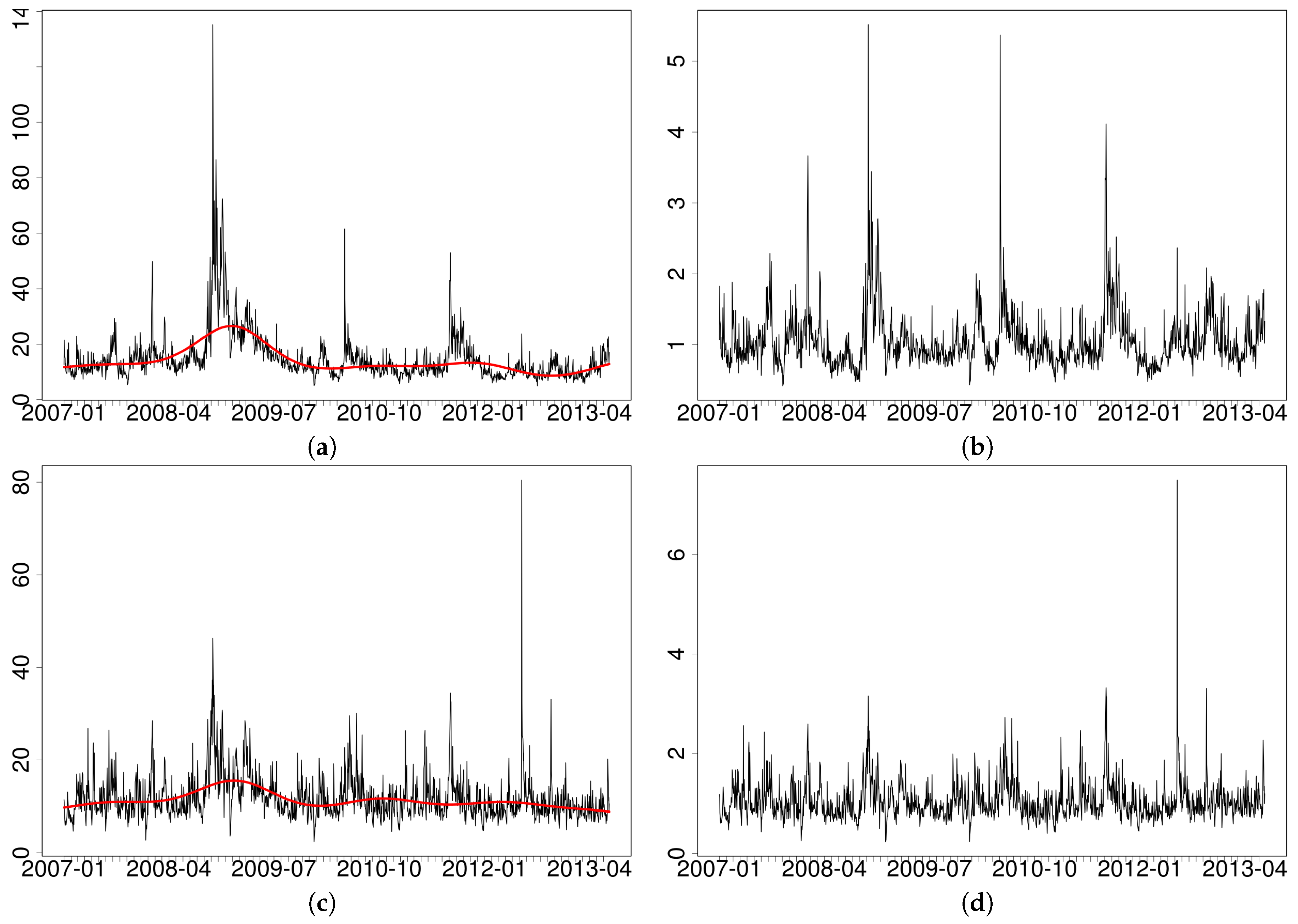
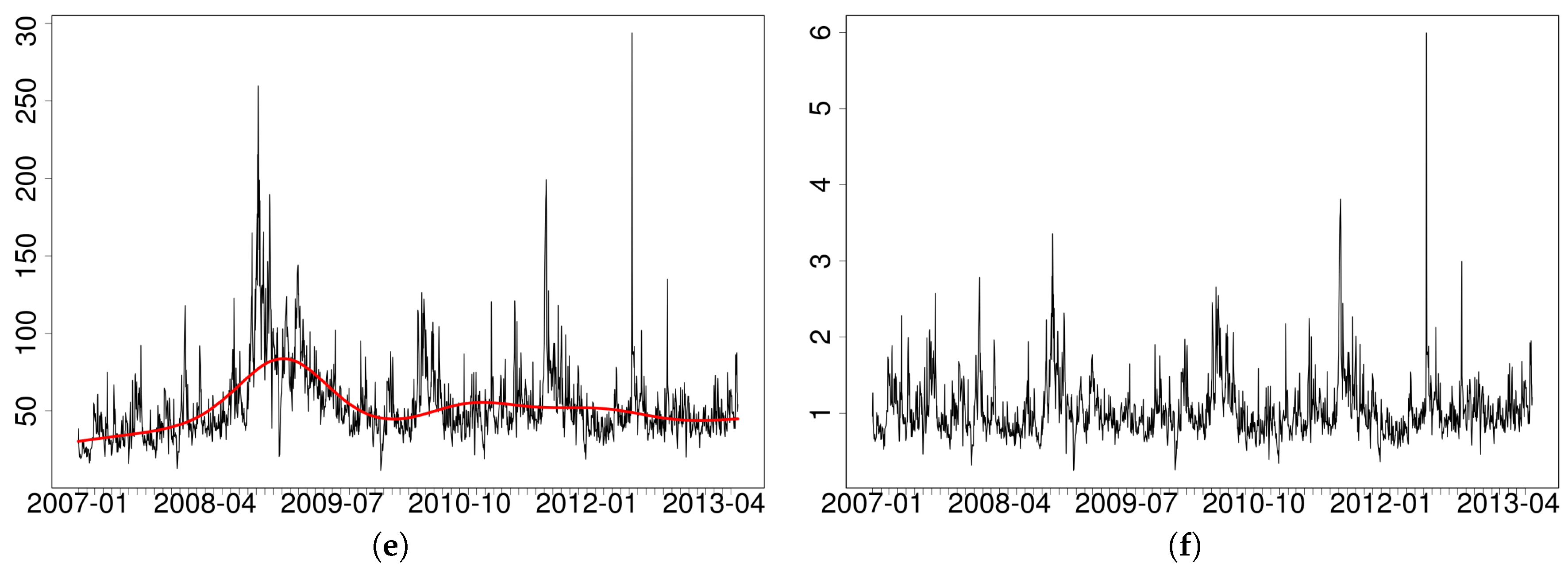
According to Figure 1, the turmoil originating with the subprime mortgage crisis is clearly affecting the profile of the series with an underlying low frequency component. For volatility, the presence of a changing average level was analyzed by Gallo and Otranto (2015) with a number of non-linear MEM’s. Without adopting their approach, in what follows we implement a filter (separately for each indicator) in order to identify short term interactions among series apart from lower frequency movements. The presence of an upward slope in the first portion of the sample is apparent and is reminiscent of the evidence produced by Andersen (1996) for volumes on an earlier period. Remarkably, this upward movement is interrupted after the peak of the crisis in October 2008, with a substantial and progressive reduction of the average level of the variables. To remove this pattern, we adopt a solution similar to Andersen (1996), that is, a flexible function of time which smooths out the series. Extracting low frequency movements in a financial market activity series with a spline is reminiscent of the stream of literature initiated by Engle and Rangel (2008) with a spline-GARCH and carried out in Brownlees and Gallo (2010) within a MEM context.

In detail, assuming that this component is multiplicative, we remove it in each indicator as follows:

• we take the log of the original series;
• we fit on each log-series a spline based regression with additive errors, using time t (a progressive counter from the first to the last observation in the sample) as an independent variable;5
• the residuals of the previous regression are then exponentiated to get the adjusted series.

When used to produce out-of-sample forecasts of the original quantities, the described approach is applied assuming that the low frequency component remains constant at the last in-sample estimate. This strategy is simple to implement and fairly reliable for forecasting at moderate horizons.

Table 1. Correlations for JNJ (3 January 2007–30 June 2013). $rkv=$ realized kernel volatility; $vol=$ volume; $nt=$ number of trades.

	Original		Low Freq. Comp.		Adjusted
	$vol$	$nt$	$vol$	$nt$	$vol$	$nt$
$rkv$	0.646	0.778	0.800	0.847	0.609	0.743
$vol$		0.890		0.780		0.932

shows some similarities across original and adjusted series, with some expected increase in the correlation between volumes and number of trades in the adjusted series (due to a smaller correlation in the corresponding low frequency components). Although still quite large overall, after adjustment, correlations are more spread apart: as mentioned, the value concerning volumes and the number of trades, above $0.9$, is the highest one; $cor(rkv,vol)$ is about $0.6$, whereas the $cor(rkv,nt)$ is still above $0.7$, all confirming the intuition that the information contained in other variables related to trading activity relevant.

5.1. Modeling Results

In the application, we consider a vMEM on adjusted data, where the conditional expectation ${\mathit{\mu }}_t$ has the form (cf. Equation (3))

$${\mathit{\mu }}_t=\mathit{\omega }+{\mathit{\alpha }}_1{\mathit{x}}_{t-1}+{\mathit{\alpha }}_2{\mathit{x}}_{t-2}+{\mathit{\gamma }}_1{\mathit{x}}_{t-1}^{(-)}+{\mathit{\beta }}_1{\mathit{\mu }}_{t-1}.$$

(44)

In order to appreciate the contribution of the different model variables, we consider alternative specifications for the coefficient matrices ${\mathit{\alpha }}_1$ and ${\mathit{\beta }}_1$ (${\mathit{\alpha }}_2$ and ${\mathit{\gamma }}_1$ are kept diagonal in all specifications), and for the error term.

As of the former, we consider specifications with both ${\mathit{\alpha }}_1$ and ${\mathit{\beta }}_1$ diagonal (labeled D); ${\mathit{\alpha }}_1$ full and ${\mathit{\beta }}_1$ diagonal (labeled A); ${\mathit{\alpha }}_1$ diagonal and ${\mathit{\beta }}_1$ full (labeled B); both ${\mathit{\alpha }}_1$ and ${\mathit{\beta }}_1$ full (labeled $AB$). For the joint distribution of the errors, we adopt a Student–T, a Normal and an Independent copula (T, N and I as respective labels), in all cases with Gamma distributed marginals. As a comparison, the $AB$ specification is also estimated by ML with log–Normal (AB-LN) and with GMM in the semiparametric AB-S. The estimated specifications are summarized in

Table 2. Estimated specifications of the vMEM defined by (1) and (44), with error distribution specified, alternatively, by (8), or (34), or (5). Notation: I for Independent copula with Gamma marginals; N for Normal copula with Gamma marginals; T for Student-T copula with Gamma marginals; $LN$ for log–Normal; S for semiparametric.

Conditional Mean (Parameters)	Error Distribution
	I	N	T	$\mathit{LN}$	S
D: ${\mathit{\alpha }}_1$, ${\mathit{\beta }}_1$, ${\mathit{\gamma }}_1$, , ${\mathit{\alpha }}_2$ diagonal	D-I
A: ${\mathit{\alpha }}_1$ full; ${\mathit{\beta }}_1$, ${\mathit{\gamma }}_1$, ${\mathit{\alpha }}_2$ diagonal	A-I	A-N	A-T
B: ${\mathit{\beta }}_1$ full; ${\mathit{\alpha }}_1$, ${\mathit{\gamma }}_1$, ${\mathit{\alpha }}_2$ diagonal		B-N	B-T
$AB$: ${\mathit{\alpha }}_1$, ${\mathit{\beta }}_1$ full; ${\mathit{\gamma }}_1$, ${\mathit{\alpha }}_2$ diagonal		AB-N	AB-T	AB-LN	AB-S

. When coupled with the conditional means in the table, the specifications with the Independent copula can be estimated equation–by–equation.

Estimation results are reported in

Table 3. Estimated coefficients of the realized volatility equation for different model formulations (cf. Table 2) for JNJ (3 January 2007–30 June 2013). Robust t-stats in parentheses. An empty space indicates that the specification did not include the corresponding coefficient. Rows labeled $vol$ and $nt$ report the p-values for causality tests (see the text for details). Overall model diagnostics report Log-likelihood values, Akaike and Bayesian Information Criteria, and p-values of a joint Ljung–Box test of no autocorrelation at various lags. Last row reports the estimation time (in seconds).

	D-I	A-I	A-N	A-T	B-N	B-T	AB-N	AB-T	AB-LN	AB-S
$rk{v}_{t-1}$	$0.4967$	$0.4575$	$0.4194$	$0.4165$	$0.4048$	$0.4019$	$0.3687$	$0.3724$	$0.3630$	$0.3777$
	($\mathit{58.10}$)	($\mathit{51.94}$)	($\mathit{48.57}$)	($\mathit{48.72}$)	($\mathit{45.25}$)	($\mathit{47.42}$)	($\mathit{39.13}$)	($\mathit{40.77}$)	($\mathit{50.76}$)	($\mathit{45.77}$)
$vo{l}_{t-1}$		$-0.0300$	$-0.0339$	$-0.0265$			$-0.0230$	$-0.0337$	$-0.0318$	$-0.0298$
		($-\mathit{1.11}$)	($-\mathit{0.97}$)	($-\mathit{0.75}$)			($-\mathit{0.54}$)	($-\mathit{0.78}$)	($-\mathit{0.93}$)	($-\mathit{0.75}$)
$n{t}_{t-1}$		$0.0668$	$0.0726$	$0.0606$			$0.1897$	$0.1890$	$0.1691$	$0.1726$
		($\mathit{1.77}$)	($\mathit{1.57}$)	($\mathit{1.36}$)			($\mathit{2.83}$)	($\mathit{2.82}$)	($\mathit{3.95}$)	($\mathit{3.51}$)
$rk{v}_{t-2}$	$-0.2672$	$-0.2485$	$-0.1878$	$-0.1923$	$-0.1950$	$-0.2054$	$-0.1778$	$-0.1827$	$-0.1811$	$-0.1790$
	($-\mathit{5.12}$)	($-\mathit{3.82}$)	($-\mathit{2.91}$)	($-\mathit{3.54}$)	($-\mathit{4.64}$)	($-\mathit{5.45}$)	($-\mathit{3.75}$)	($-\mathit{4.19}$)	($-\mathit{5.46}$)	($-\mathit{4.64}$)
$rk{v}_{t-1}^{(-)}$	$0.0252$	$0.0266$	$0.0265$	$0.0308$	$0.0255$	$0.0297$	$0.0171$	$0.0223$	$0.0211$	$0.0222$
	($\mathit{0.79}$)	($\mathit{0.79}$)	($\mathit{0.83}$)	($\mathit{1.00}$)	($\mathit{0.94}$)	($\mathit{1.13}$)	($\mathit{0.41}$)	($\mathit{0.53}$)	($\mathit{0.73}$)	($\mathit{0.67}$)
${\mu }_{t-1}^{(rkv)}$	$0.7223$	$0.7067$	$0.6793$	$0.6918$	$0.7235$	$0.7410$	$0.7588$	$0.7675$	$0.7626$	$0.7428$
	($\mathit{14.19}$)	($\mathit{9.94}$)	($\mathit{9.49}$)	($\mathit{11.41}$)	($\mathit{17.23}$)	($\mathit{20.73}$)	($\mathit{14.13}$)	($\mathit{16.46}$)	($\mathit{19.22}$)	($\mathit{15.50}$)
${\mu }_{t-1}^{(vol)}$					$-0.0317$	$-0.0139$	$-0.1138$	$-0.0466$	$-0.0909$	$-0.0938$
					($-\mathit{0.68}$)	($-\mathit{0.32}$)	($-\mathit{0.96}$)	($-\mathit{0.44}$)	($-\mathit{0.95}$)	($-\mathit{0.86}$)
${\mu }_{t-1}^{(nt)}$					$0.0492$	$0.0297$	$-0.0984$	$-0.1568$	$-0.0867$	$-0.0839$
					($\mathit{0.99}$)	($\mathit{0.66}$)	($-\mathit{0.76}$)	($-\mathit{1.26}$)	($-\mathit{0.87}$)	($-\mathit{0.73}$)
$vol$		0.2658	0.3296	0.4558	0.4970	0.7459	0.1705	0.2717	0.0853	0.1550
$nt$		0.0766	0.1153	0.1724	0.3202	0.5098	0.0051	0.0077	0.0001	0.0004
logLik	205.53	239.75	2012.39	2086.31	1967.02	2048.80	2045.81	2125.12	2153.79
AIC	−375.07	$-431.49$	$-3970.78$	−4116.61	−3880.05	−4041.60	$-4025.62$	$-4182.23$	$-4241.57$
BIC	$-258.11$	$-275.55$	$-3795.35$	$-3934.69$	$-3704.62$	$-3859.67$	−3811.20	−3961.32	$-4027.16$
LB(12)	0.0000	0.0000	0.0001	0.0001	0.0000	0.0000	0.0388	0.0141	0.0450	0.0596
LB(22)	0.0000	0.0000	0.0000	0.0000	0.0000	0.0000	0.0178	0.0109	0.0229	0.0264
LB(32)	0.0000	0.0000	0.0003	0.0003	0.0000	0.0000	0.0192	0.0132	0.0291	0.0267
time	0.342	0.753	2.628	15.044	2.485	14.707	2.714	14.859	0.155	0.132

, limiting ourselves to the equation for the realized volatility.6 Among copula-based specifications, the Student-T copula turns out to be the favorite version, judging upon a significantly higher log–likelihood function value, and lower information criteria;7 the equation–by–equation approach (Independent copula) is dominated in both respects.8

An estimation of the Diagonal model with the Normal/Student-T copula function (details not reported) shows log-likelihood values of $1947.91$, respectively, $2034.07$ (relative to the base value of $205.53$ in the first column), pointing to both a substantial improvement coming from the contemporaneous correlation of the innovations and to the joint significance of the other indicators when the A specification is adopted. The comparison of the A (${\mathit{\alpha }}_1$ full; ${\mathit{\beta }}_1$ and ${\mathit{\gamma }}_1$ diagonal) versus the B (${\mathit{\beta }}_1$ full; ${\mathit{\alpha }}_1$ and ${\mathit{\gamma }}_1$ diagonal) formulations, seems to indicate a dominance of the former, at least judging upon the overall log-likelihood values. It is also interesting to note that model residual autocorrelation is substantially reduced only in the case of richer parameterizations ($AB$), where non–diagonality in both ${\mathit{\alpha }}_1$ and ${\mathit{\beta }}_1$ captures possible interdependencies, with a sharp improvement in the LB diagnostics (although only marginally satisfying).

In general, it seems that the more relevant contribution in determining realized volatility comes from the lagged number of trades, but only in the $AB$ models (some collinearity effect, diminishing individual significance, is to be expected); the relevance of such information is also highlighted by the Granger Causality tests, to check whether lagged model components attributable to either $vol$ or $nt$ have joint significance. In detail, using three indices where the first refers to the LHS variable, the second to the conditioning variable, and the third the lag, we test $H_0:{\alpha }_{1,j,1}=0$ ($j=2,3$) in the A-based formulations; $H_0:{\beta }_{1,j,1}=0$ ($j=2,3$) in the B-based formulations; $H_0:{\alpha }_{1,j,1}={\beta }_{1,j,1}=0$ ($j=2,3$) in the $AB$-based formulations.

The own volatility coefficients at lag 2 are always significant (with negative signs); surprisingly, the leverage effect related to the sign of the returns is not.

The Normal and the Student-T specifications appear to provide similar point estimates, except for the non-diagonal $\beta$ coefficients: for the latter, once again, the picture may be clouded by collinearity, since a formal log–likelihood test does indicate joint significance.9

The overview of the estimation results is complete by examining the

Table 4. Square root of the estimated elements on the main diagonal of $\mathsf{\Sigma }$ (cf. Equation (5)).

	D-I	A-I	A-N	A-T	B-N	B-T	AB-N	AB-T	AB-LN	AB-S
${\sigma }_1$	0.209	0.208	0.207	0.212	0.209	0.214	0.206	0.210	0.204	0.226
${\sigma }_2$	0.254	0.251	0.252	0.256	0.257	0.262	0.252	0.256	0.252	0.272
${\sigma }_3$	0.227	0.227	0.229	0.236	0.232	0.240	0.228	0.235	0.228	0.242

, where we report the square root of the estimated elements on the main diagonal of $\mathsf{\Sigma }$ for all specifications, showing substantial similarity.

Finally, the correlation coefficients implied by the various specifications are reported in

Table 5. Estimated correlation matrices of the copula functions (specifications -N and -T), and of ${\mathit{\epsilon }}_t$ (specifications -LN and -S).

	A-N		A-T		AB-N		AB-T		AB-LN		AB-S
	${\mathit{vol}}_{\mathit{t}}$	${\mathit{nt}}_{\mathit{t}}$	${\mathit{vol}}_{\mathit{t}}$	${\mathit{nt}}_{\mathit{t}}$	${\mathit{vol}}_{\mathit{t}}$	${\mathit{nt}}_{\mathit{t}}$	${\mathit{vol}}_{\mathit{t}}$	${\mathit{nt}}_{\mathit{t}}$	${\mathit{vol}}_{\mathit{t}}$	${\mathit{nt}}_{\mathit{t}}$	${\mathit{vol}}_{\mathit{t}}$	${\mathit{nt}}_{\mathit{t}}$
$rk{v}_t$	0.483	0.610	0.505	0.626	0.485	0.612	0.505	0.628	0.469	0.596	0.481	0.605
$vo{l}_t$		0.902		0.917		0.903		0.918		0.902		0.906

, showing that a strong correlation among innovations further supports the need for taking simultaneity into account.

The alternative log–Normal and Semiparametric formulations deliver parameter inferences qualitatively similar to the corresponding versions based on copulas. The AIC and BIC statistics of the log–Normal are better than the copula based formulations (for the semiparametric they are not available); also its Ljung-Box diagnostics are marginally better.

A comparison of the estimation times across specifications10 reveals some differences. Student-T copula based formulations are the slowest; the Normal copula based estimated with the concentrated likelihood approach takes about 1/6 of time; finally, the log–Normal and the Semiparametric are a lot faster (about 1/20 of the Normal based). Differences notwithstanding, the largest times involved are very low on an absolute scale.

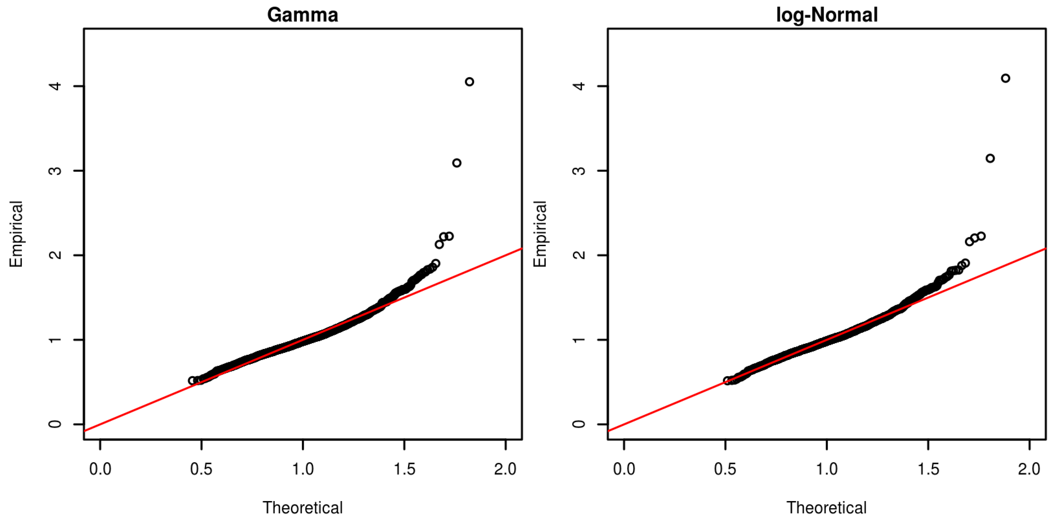
Figure 2 shows a comparison between the estimated residuals against their theoretical counterparts in the case of the Gamma and log–Normal distributions. In both cases, the fit seems to break apart for the tail of the distribution, pointing to the need for some care about the evolution of volatility of volatility (a mixture of distribution hypothesis is contemplated in, say, De Luca and Gallo (2009) in a MEM model).

5.2. Forecasting

We left the period 1 July–31 December 2013 (128 observations) for out–of–sample forecasting comparisons. We adopt a Diebold and Mariano (1995) test statistic for superior predictive ability using the error measures

$$e_{N,t}=\frac{1}{2}{(x_t-{\mu }_t)}^2{e}_{G,t}=\frac{x_t}{{\mu }_t}-1-ln\left(\frac{x_t}{{\mu }_t}\right).$$

(45)

where $x_t$ and ${\mu }_t$ denote here the observed and the predicted values, respectively. $e_{N,t}$ is the squared error, and can be interpreted as the loss behind an $x_t$ Normally distributed with mean ${\mu }_t$; similarly, $e_{G,t}$ can be interpreted as the loss we can derive considering $x_t$ as Gamma distributed with mean ${\mu }_t$ and variance proportional to ${\mu }_t^2$. Comparisons are performed on both Original and Adjusted (i.e., removing the low frequency component) series.

Table 6. Diebold-Mariano test statistics for unidirectional comparisons, against the AB-T specification, considering 1-step ahead forecasts (out–of–sample period 1 July–31 December 2013). The error measures are defined as $e_{N,t}=0.5{(x_t-{\mu }_t)}^2$ (Normal loss) and $e_{G,t}=x_t/{\mu }_t-1-ln(x_t/{\mu }_t)$ (Gamma loss), where $x_t$ and ${\mu }_t$ denote the observed and the predicted values, respectively (cf. Section 5.2 for the interpretation). Boldface (italic) indicates 5% (10%) significant statistics.

Specification	${\mathit{e}}_{\mathit{N},\mathit{t}}$		${\mathit{e}}_{\mathit{G},\mathit{t}}$
	Adjusted	Original	Adjusted	Original
D-I	−2.490	−2.107	−2.428	−2.132
A-I	−1.358	−1.200	−1.277	−1.173
A-N	$-0.668$	−0.621	−0.563	−0.591
A-T	$-0.510$	−0.449	−0.422	−0.431
B-N	$-0.553$	−0.557	$-0.449$	−0.560
B-T	$-0.474$	−0.479	−0.389	−0.490
AB-N	$-0.768$	−0.757	$-0.737$	−0.708
AB-LN	0.868	0.720	0.980	0.742
AB-S	$-0.277$	$-0.230$	$-0.180$	$-0.164$

reports the values of the Diebold-Mariano test statistic of different model formulations, against the AB-T specification (which has the lowest values of the information criteria among copula-based specifications, cf. Table 3), considering one-step ahead predictions.

There are no substantial differences in performance between the results on the original and the adjusted series.11 We notice a definite improvement of the specification involving simultaneous innovations over the equation–by–equation specifications (first two rows). The Student–T Copula improves upon the Normal formulation (marginally, line AB-N), but is substantially equivalent to the AB-LN (slightly better) and the AB-S (slightly worse).

6. Conclusions

The Multiplicative Error Model was originally introduced by Engle (2002) as a positive valued product process between a scale factor following a GARCH type dynamics and a unit mean innovation process. In this paper we have presented a general discussion of a vector extension of such a model with a dynamically interdependent formulation for the scale factors where lagged variables and conditional expectations may be both allowed to impact each other’s conditional mean. Engle and Gallo (2006) estimate a vMEM where the innovations are Gamma–distributed with a diagonal variance–covariance matrix (estimated equation–by-equation). The extension to a truly multivariate process requires a complete treatment of the interdependence among the innovation terms. One possibility is to avoid the specification of the distribution and adopt a semiparametric GMM approach as in Cipollini et al. (2013). In this paper we have derived a maximum likelihood estimator by framing the innovation vector as a copula function linking Gamma marginals; a parametric alternative with a multivariate log-Normal distribution is discussed, while we show that the specification using a multivariate Gamma distribution has severe shortcomings.

We illustrate the procedure on three indicators related to market trading activity: realized volatility, volumes, and number of trades. The empirical results are presented in reference to daily data on the Johnson and Johnson (JNJ) stock. The data on the three variables show a (slowly moving) time varying local average which was removed before estimating the parameters. The three components are highly correlated with one another, but interestingly, their removal does not have a substantial impact on the correlation among the adjusted series. The specifications adopted start from a diagonal structure where no dynamic interaction is allowed, and an Independent copula (de facto an equation–by–equation specification). Refinements are obtained by inserting a Normal copula and a Student–T copula (which dramatically improve the estimated log–likelihood function values) and then allowing for the presence of dynamic interdependence in the form of links either between lagged variables, or between lagged conditional means, or both. Although hindered by the presence of some collinearity, the results clearly show a significant improvement for the fit of the equation for realized volatility when volumes and number of trades are considered. This is highlighted by significantly better model log–likelihoods, lower overall information criteria and improved autocorrelation diagnostics. The results of an out–of–sample forecasting exercise confirm the need for a simultaneous approach to model specification and estimation, with a substantial preference for the Student-T copula results within the copula–based formulations. From a interpretive point of view, the results show that the past realized volatility is not enough information by itself to reconstruct the dynamics: its modeling and forecastability are clearly influenced by other indicators of market trading activity, and simultaneous correlations in the innovations must be accounted for.

Under equal models for conditional means, the copula approach is substantially equivalent to other forms of specifications, be they parametric with a multivariate log-Normal error, or semiparametric (with GMM estimation). The advantage of a slightly more expensive (from a computational point of view) procedure lies in gaining flexibility in the tail dependence offered by the Student–T copula, which can be a plus when reconstructing joint conditional distributions, or when reproducing more realistic behavior in simulation is desirable.

References

1. Andersen, Torben G. 1996. Return Volatility and Trading Volume: An Information Flow Interpretation of Stochastic Volatility. The Journal of Finance 51: 169–204. [Google Scholar] [CrossRef]
2. Andersen, Torben G., Tim Bollerslev, Peter F. Christoffersen, and Francis X. Diebold. 2006. Volatility and Correlation Forecasting. In Handbook of Economic Forecasting. Edited by Graham Elliott, Clive W.J. Granger and Allan Timmermann. New York: North Holland, pp. 777–878. [Google Scholar]
3. Barndorff-Nielsen, Ole E., Peter Reinhard Hansen, Asger Lunde, and Neil Shephard. 2009. Realised kernels in Practice: trades and quotes. Econometrics Journal 12: 1–32. [Google Scholar] [CrossRef]
4. Barndorff-Nielsen, Ole E., Peter Reinhard Hansen, Asger Lunde, and Neil Shephard. 2011. Multivariate realised kernels: Consistent positive semi-definite estimators of the covariation of equity prices with noise and non-synchronous trading. Journal of Econometrics 162: 149–69. [Google Scholar] [CrossRef]
5. Bodnar, Taras, and Nikolaus Hautsch. 2016. Dynamic conditional correlation multiplicative error processes. Journal of Empirical Finance 36: 41–67. [Google Scholar] [CrossRef]
6. Bollerslev, Tim. 1986. Generalized Autoregressive Conditional Heteroskedasticity. Journal of Econometrics 31: 307–27. [Google Scholar] [CrossRef]
7. Bouyé, Eric, Valdo Durrleman, Ashkan Nikeghbali, Gaël Riboulet, and Thierry Roncalli. 2000. Copulas for Finance: A Reading Guide and Some Applications. Technical Report. Credit Lyonnais, Paris: Groupe de Recherche Opérationelle. [Google Scholar]
8. Brownlees, Christian T., and Giampiero M. Gallo. 2006. Financial Econometric Analysis at Ultra–High Frequency: Data Handling Concerns. Computational Statistics and Data Analysis 51: 2232–45. [Google Scholar] [CrossRef]
9. Brownlees, Christian T., and Giampiero M. Gallo. 2010. Comparison of Volatility Measures: A Risk Management Perspective. Journal of Financial Econometrics 8: 29–56. [Google Scholar] [CrossRef]
10. Cerrato, Mario, John Crosby, Minjoo Kim, and Yang Zhao. 2015. Modeling Dependence Structure and Forecasting Market Risk with Dynamic Asymmetric Copula. Technical Report. Glasgow, Scotland: Adam Smith Business School, University of Glasgow. [Google Scholar]
11. Cherubini, Umberto, Elisa Luciano, and Walter Vecchiato. 2004. Copula Methods in Finance. New York: Wiley. [Google Scholar]
12. Chou, Ray Yeutien. 2005. Forecasting Financial Volatilities with Extreme Values: The Conditional Autoregressive Range (CARR) Model. Journal of Money, Credit and Banking 37: 561–82. [Google Scholar] [CrossRef]
13. Cipollini, Fabrizio, and Giampiero M. Gallo. 2010. Automated variable selection in vector multiplicative error models. Computational Statistics & Data Analysis 54: 2470–86. [Google Scholar] [CrossRef]
14. Cipollini, Fabrizio, Robert F. Engle, and Giampiero M. Gallo. 2013. Semiparametric Vector MEM. Journal of Applied Econometrics 28: 1067–86. [Google Scholar] [CrossRef]
15. De Luca, Giovanni, and Giampiero M. Gallo. 2009. Time-varying Mixing Weights in Mixture Autoregressive Conditional Duration Models. Econometric Reviews 28: 102–20. [Google Scholar] [CrossRef]
16. Demarta, Stefano, and Alexander J. McNeil. 2005. The t Copula and Related Copulas. International Statistical Review 73: 111–29. [Google Scholar] [CrossRef]
17. Diebold, Francis X., and Roberto S. Mariano. 1995. Comparing Predictive Accuracy. Journal of Business & Economic Statistics 13: 253–63. [Google Scholar] [CrossRef]
18. Embrechts, Paul, Alexander McNeil, and Daniel Straumann. 2002. Correlation and dependence in risk management: properties and pitfalls. In Risk Management: Value at Risk and Beyond. Edited by M. A. H. Dempster. Cambridge: Cambridge University Press, pp. 176–223. [Google Scholar]
19. Engle, Robert F. 2002. New Frontiers for ARCH Models. Journal of Applied Econometrics 17: 425–46. [Google Scholar] [CrossRef]
20. Engle, Robert F., and Giampiero M. Gallo. 2006. A Multiple Indicators Model for Volatility Using Intra-Daily Data. Journal of Econometrics 131: 3–27. [Google Scholar] [CrossRef]
21. Engle, Robert F., and Jeffrey R. Russell. 1998. Autoregressive Conditional Duration: A New Model for Irregularly Spaced Transaction Data. Econometrica 66: 1127–62. [Google Scholar] [CrossRef]
22. Engle, Robert F., and Joe Mezrich. 1995. Grappling with GARCH. Risk 8: 112–17. [Google Scholar]
23. Engle, Robert F., and Jose Gonzalo Rangel. 2008. The Spline-GARCH Model for Low Frequency Volatility and Its Global Macroeconomic Causes. Review of Financial Studies 21: 1187–222. [Google Scholar] [CrossRef]
24. Frahm, Gabriel, Markus Junker, and Alexander Szimayer. 2003. Elliptical Copulas: Applicability and Limitations. Statistics & Probability Letters 63: 275–86. [Google Scholar] [CrossRef]
25. Francq, Christian, Lajos Horvath, and Jean-Michel Zakoïan. 2011. Merits and drawbacks of variance targeting in GARCH models. Journal of Financial Econometrics 9: 619–56. [Google Scholar] [CrossRef]
26. Gallo, Giampiero M., and Edoardo Otranto. 2015. Forecasting realized volatility with changing average levels. International Journal of Forecasting 31: 620–34. [Google Scholar] [CrossRef]
27. Hamilton, James Douglas. 1994. Time Series Analysis. Princeton: Princeton University Press. [Google Scholar]
28. Hautsch, Nikolaus. 2008. Capturing common components in high-frequency financial time series: A multivariate stochastic multiplicative error model. Journal of Economic Dynamics and Control 32: 3978–4015. [Google Scholar] [CrossRef]
29. Hautsch, Nikolaus, Peter Malec, and Melanie Schienle. 2013. Capturing the Zero: A New Class of Zero-Augmented Distributions and Multiplicative Error Processes. Journal of Financial Econometrics 12: 89–121. [Google Scholar] [CrossRef]
30. Horváth, Lajos, Piotr Kokoszka, and Ricardas Zitikis. 2006. Sample and Implied Volatility in GARCH Models. Journal of Financial Econometrics 4: 617–35. [Google Scholar] [CrossRef]
31. Joe, Harry. 1997. Multivariate Models and Dependence Concepts. London: Chapman & Hall. [Google Scholar]
32. Johnson, Norman L., Samuel Kotz, and Narayanaswamy Balakrishnan. 2000. Continuous Multivariate Distributions. New York: John Wiley & Sons, vol. 1. [Google Scholar]
33. Kostadinov, Krassimir. 2005. Non-parametric Estimation of Elliptical Copulae with Application to Credit Risk. Technical Report. Munich, Germany: Munich University of Technology. [Google Scholar]
34. Kristensen, Dennis, and Oliver Linton. 2004. Consistent Standard Errors for Target Variance Approach to GARCH Estimation. Econometric Theory 20: 990–93. [Google Scholar] [CrossRef]
35. Lindskog, Filip, Alexander McNeil, and Uwe Schmock. 2003. Kendall’s tau for elliptical distributions. In Credit Risk: Measurement, Evaluation and Management. Edited by Georg Bol, Gholamreza Nakhaeizadeh, Svetlozar T. Rachev, Thomas Ridder and Karl-Heinz Vollmer. Heidelberg: Physica-Verlag. [Google Scholar]
36. Manganelli, Simone. 2005. Duration, Volume and Volatility Impact of Trades. Journal of Financial Markets 8: 377–99. [Google Scholar] [CrossRef]
37. McNeil, Alexander J., Rüdiger Frey, and Paul Embrechts. 2005. Quantitative Risk Management: Concepts, Techniques, and Tools. Princeton: Princeton University Press. [Google Scholar]
38. Nelsen, Roger B. 1999. An introduction to Copulas. Lecture Notes in Statistics. New York: Springer. [Google Scholar]
39. Newey, Whitney K., and Daniel McFadden. 1994. Large sample estimation and hypothesis testing. In Handbook of Econometrics. Edited by Robert Engle and Dan McFadden. New York: Elsevier, vol. 4, chapter 36. pp. 2111–45. [Google Scholar]
40. Nocedal, Jorge, and Stephen J. Wright. 2006. Numerical Optimization. Springer Series in Operations Research and Financial Engineering; Berlin: Springer. [Google Scholar]
41. Noss, Joseph. 2007. The Econometrics of Optimal Execution in an Order-Driven Market. Master’s dissertation, Nuffield College, Oxford University, Oxford, UK. [Google Scholar]
42. Okimoto, Tatsuyoshi. 2008. New Evidence of Asymmetric Dependence Structures in International Equity Markets. The Journal of Financial and Quantitative Analysis 43: 787–815. [Google Scholar] [CrossRef]
43. Patton, Andrew J. 2006. Modelling asymmetric exchange rate dependence. International Economic Review 47: 527–56. [Google Scholar] [CrossRef]
44. Patton, Andrew J. 2013. Copula Methods for Forecasting Multivariate Time Series. In Handbook of Economic Forecasting. Edited by Graham Elliott and Allan Timmermann. New York: Elsevier, vol. 2, Part B. pp. 899–960. [Google Scholar]
45. Powell, Michael J.D. 2006. The NEWUOA software for unconstrained optimization without derivatives. In Large-Scale Nonlinear Optimization. Edited by Gianni D. Pillo and Massimo Roma. New York: Springer Verlag, pp. 255–97. [Google Scholar]
46. Schmidt, Rafael. 2002. Tail dependence for elliptically contoured distributions. Mathematical Methods of Operations Research 55: 301–27. [Google Scholar] [CrossRef]
47. Song, Peter Xue-Kun. 2000. Multivariate Dispersion Models Generated From Gaussian Copula. Scandinavian Journal of Statistics 27: 305–20. [Google Scholar] [CrossRef]
1
In some applications, especially involving returns, their elliptical symmetry may constitute a limit (cf., for example, Patton (2006), Okimoto (2008), Cerrato et al. (2015) and reference therein). Copulas in the Archimedean family (Clayton, Gumbel, Joe-Clayton, etc.) offer a way to bypass such a limitation but suffer from other drawbacks and, in any case, seem to be less relevant for the variables of interest for a vMEM (here, different indicators of trading activity). They will not be pursued in what follows.
2
This is equivalent to variance targeting in a GARCH context (Engle and Mezrich 1995), where the constant term of the conditional variance model is assumed to be a function of the sample unconditional variance and of the other parameters. In this context, other than a preference for the term expectation targeting since we are modeling a conditional mean, the main argument stays unchanged.
3
Even when R is a ( 2 , 2 ) matrix, the value of R 12 has to satisfy the cubic equation:
R 12 3 R 12 2 q 1 q 2 T + R 12 q 1 q 1 T + q 2 q 2 T 1 q 1 q 2 T = 0 .
4
(40) and (41) come from standard properties of the multivariate Normal distribution: the former is implied by the fact that all centered odd moments of ln ε t are zero; the latter is implied by the structure of fourth centered moments of ln ε t .
5
Alternative methods, such as a moving average of fixed length (centered or uncentered), can be used but in practice they deliver very similar results and will not be discussed in detail here. The spline regression is estimated with the gam() function in the R package mgcv by using default settings.
6
All models are estimated using Expectation Targeting (Section 3.2.1). The Normal copula based specifications are estimated resorting to the concentrated log-likelihood approach (Section 3.2.2). We omit estimates of the constant term ω .
7
The estimated degrees of freedom are 8.53 (s.e. 1.16 ) and 8.18 (s.e. 1.05 ), respectively, in the A-T and AB-T formulations. We also tried full ML estimation of the AB-N specification getting a value of the log-likelihood equal to 2046.57 , very close to the concentrated log-likelihood approach (Section 3.2.2) used in Table 3.
8
The stark improvement in the likelihood functions, coming from the explicit consideration of the correlation structure, does not guarantee similar gains in the forecasting ability of the same variables. This is similar to what happens in modeling returns, when the likelihood function of ARMA models is improved by superimposing a GARCH structure on the conditional variances: no substantive change in the fit of the conditional mean and no better predictive ability.
9
No attempt at pruning the structure of the model following the automated procedure suggested in Cipollini and Gallo (2010) was performed.
10
Calculations with our routines written in R were performed on an Intel i7-5500U 2.4Ghz processor. We did not perform an extensive comparison of estimation times and we did not optimize performance by removing tracing of intermediate results. Moreover, the copula-based and the alternative specifications are optimized resorting to different algorithms: the first ones, more cumbersome to optimize, are estimated toward a combination of NEWUOA (Powell 2006) and Newton-Raphson; for the second ones we used a dogleg algorithm (Nocedal and Wright 2006, ch. 4).
11
One-step ahead predictions at time t for the original series are computed multiplying the corresponding forecast of the adjusted indicator by the value of the low frequency component at t 1 .
Figure 1. Time series of the trading activity indices for JNJ (3 January 2007–30 June 2013). (a,c,e) original data; (b,d,f) data after removing the low frequency component. (a,b) realized kernel volatility (annualized percentage); (c,d) volumes (millions); (e,f) number of trades (thousands). The spike on 13 June 2012 corresponds to an important acquisition and a buy back of some of its common stock by a subsidiary.
Econometrics 05 00016 g001aEconometrics 05 00016 g001b
Figure 2. QQ-plot between theoretical and empirical residuals for the realized volatility of JNJ. Comparison with Gamma and log–Normal distributions. Estimation period: 3 January 2007– 30 June 2013.
Econometrics 05 00016 g002