Fiscal Multipliers in a Diversifying Economy: Comparing Government Consumption and Infrastructure Investment Effects on Non-Oil GDP in Saudi Arabia a Quarterly SVAR Analysis

Abstract

Saudi Arabia’s Vision 2030 aims to diversify the economy away from oil by reallocating public expenditure from current consumption toward infrastructure mega-projects. This research estimates and compares the fiscal multipliers of government consumption and government investment on non-oil GDP using quarterly data from 2010Q2 to 2026Q1. A vector error correction model with Cholesky identification is employed alongside local projections to ensure robustness. Results indicate that the investment multiplier is substantially larger and more persistent than the consumption multiplier, reaching 2.34 after twelve quarters compared to 0.58 for consumption. A structural break analysis reveals that multipliers have increased markedly since 2016, with the eight-quarter investment multiplier rising from 1.24 pre-Vision 2030 to 2.61 thereafter. Variance decomposition confirms that government investment shocks explain over 27% of non-oil output fluctuations at longer horizons, independent of oil price movements. These findings provide empirical support for the strategic emphasis on capital formation under Vision 2030 and suggest that prioritising infrastructure investment over current expenditure yields superior growth dividends in a diversifying oil economy.

1. Introduction

The effectiveness of fiscal policy in stimulating economic activity remains a central question in macroeconomics, particularly in the aftermath of the 2008 global financial crisis and the COVID-19 pandemic, which prompted unprecedented government spending across the world. The fiscal multiplier—the change in output resulting from a one-unit change in government expenditure—has been extensively studied, yet estimates vary widely depending on country characteristics, the type of spending, the state of the business cycle, and the methodological approach employed (Blanchard & Perotti, 2002; Ramey, 2011; Auerbach & Gorodnichenko, 2012; Ilzetzki et al., 2013). A robust consensus emerging from this literature is that government investment, particularly in infrastructure, tends to generate larger and more persistent multipliers than government consumption, especially in economies with slack and well-developed implementation capacity (Abiad et al., 2016; IMF, 2014). However, the empirical evidence remains heavily skewed toward advanced economies and a handful of large emerging markets, leaving significant gaps in our understanding of fiscal transmission in resource-dependent and diversifying economies.

For oil-exporting countries, the analysis of fiscal multipliers is complicated by several distinctive features. First, these economies often operate fixed exchange rate regimes, which dampen the monetary policy offset and can amplify the effects of fiscal shocks (Ilzetzki et al., 2013). Second, the dominance of the hydrocarbon sector introduces a large exogenous revenue source that can weaken the link between domestic taxation and spending, potentially altering private sector expectations (Behar & Fouejieu, 2018; Arezki & Blanchard, 2014). Third, the public sector’s role as the primary engine of non-oil growth means that fiscal policy is not merely a stabilisation tool but a structural driver of economic diversification (Cherif & Hasanov, 2019). Studies focusing on Gulf Cooperation Council (GCC) countries have found that fiscal multipliers are generally small in the short run but can be substantial over longer horizons, especially when spending is directed toward capital formation (Kandil & Morsy, 2011; Al-Eyd & Barrell, 2005). Yet, most of this work relies on annual data or aggregate spending measures, obscuring the potentially heterogeneous effects of different spending categories.

Saudi Arabia presents a compelling case study at the intersection of these debates. As the largest economy in the GCC and the world’s leading oil exporter, the Kingdom has long relied on hydrocarbon revenues to finance a generous public sector wage bill and extensive social transfers. However, the launch of Vision 2030 in 2016 marked a fundamental shift in fiscal strategy. Under this ambitious reform agenda, the government has committed to reducing the economy’s dependence on oil by fostering a vibrant non-oil private sector, partly through a reallocation of public expenditure away from current consumption (such as public sector salaries and subsidies) and toward transformative infrastructure mega-projects—including NEOM, the Red Sea Project, and Qiddiya—as well as investments in renewable energy, tourism, and logistics (Saudi Vision 2030, 2016; IMF, 2023). This policy pivot raises a critical empirical question: does the composition of government spending matter for non-oil growth in Saudi Arabia, and if so, to what extent? Answering this question is essential for guiding budget allocation and assessing the growth implications of Vision 2030’s fiscal reforms.

Despite its policy relevance, empirical evidence on the relative efficacy of government consumption versus investment in Saudi Arabia remains scarce. Existing studies for the Kingdom either employ aggregated spending data, pre-date the Vision 2030 era, or focus on the aggregate fiscal stance rather than the composition of expenditure (Joharji & Starr, 2011; Al-Fawwaz, 2016; Iqbal & Nader, 2024). Moreover, the availability of quarterly real GDP disaggregated by economic activity and expenditure components—recently published by the General Authority for Statistics—now permits a more granular and timely analysis than was previously possible. To our knowledge, no study has yet exploited this quarterly data to estimate and compare the multipliers of government consumption and infrastructure investment on non-oil output in Saudi Arabia within a unified structural framework.

This paper addresses this gap by asking the following question: do government expenditures on current consumption (government services) and infrastructure investment (gross fixed capital formation) have significantly different multiplier effects on non-oil GDP in Saudi Arabia? We pursue four specific objectives. First, we estimate the short-run and long-run fiscal multipliers for both government consumption and government investment using structural vector autoregression (SVAR) with Cholesky identification and a vector error correction model (VECM) that accounts for cointegration among the key variables. Second, we test whether the investment multiplier is larger and more persistent than the consumption multiplier. Third, we examine whether these multipliers have changed after the launch of Vision 2030 by conducting a structural break analysis and estimating rolling-window multipliers. Fourth, we assess the robustness of our findings using the local projection method of Ò. Jordà (2005), which imposes fewer parametric restrictions and is less sensitive to model misspecification.

Our analysis employs quarterly data from 2010Q2 to 2026Q1 for nine variables: real non-oil GDP, real government GDP (a proxy for consumption), real gross fixed capital formation (a proxy for investment), real oil GDP, the oil price deflator, real private GDP, real exports, real imports, and real utility GDP. The main model is a five-variable VECM identified recursively, with the ordering based on the assumed contemporaneous exogeneity of oil price and output shocks relative to fiscal variables. The results provide the first rigorous, composition-specific fiscal multiplier estimates for Saudi Arabia in the Vision 2030 era.

The remainder of the paper is organised as follows. Section 2 contains a literature review with a theoretical framework. Section 3 outlines the empirical methodology, describes the data and presents descriptive statistics including unit root and cointegration tests, the VECM specification, and the local projection approach. Section 4 reports the main results, including impulse response functions, multiplier estimates, variance decompositions, and the structural break analysis. Section 5 offers a discussion of the findings and their policy implications. Section 6 concludes the paper.

2. Literature Review and Theoretical Framework

The study of fiscal multipliers—the change in output resulting from an exogenous shift in government expenditure—occupies a central position in macroeconomic research and policymaking. Since the seminal contribution of Blanchard and Perotti (2002), who introduced the structural vector autoregression (SVAR) methodology with institutional identification to isolate fiscal shocks, a substantial empirical literature has sought to quantify the size and determinants of these multipliers. Their identification scheme, which exploits the delayed legislative and implementation lags inherent in fiscal policy, established the standard framework for estimating the dynamic effects of government spending on output, and has been widely adopted across both advanced and developing economies (Blanchard & Perotti, 2002). Subsequent research has revealed that the magnitude of the fiscal multiplier is not a universal constant but depends critically on a constellation of structural characteristics, including the composition of spending. Barnichon et al. (2022) demonstrated that contractionary government spending shocks generate substantially larger multiplier effects than expansionary shocks, particularly during periods of economic slack, depending on the monetary policy regime, the degree of trade openness, and the position of the economy within the business cycle (Ilzetzki et al., 2013; Auerbach & Gorodnichenko, 2012).

2.1. Theoretical Foundations and the Composition of Public Expenditure

A central theoretical question concerns whether the composition of government expenditure—specifically, the distinction between government consumption (current purchases of goods and services, including public sector wages) and government investment (capital formation, particularly infrastructure)—matters for the magnitude and persistence of the fiscal multiplier. Kasasbeh (2025) found that the Public Investment Fund (PIF) has significantly contributed to Saudi Arabia’s economic diversification, foreign direct investment inflows, and overall financial performance. Neoclassical and New Keynesian models offer divergent predictions regarding this composition effect. Standard New Keynesian dynamic stochastic general equilibrium (DSGE) models, which feature nominal rigidities and imperfect competition, typically predict that both forms of government spending can stimulate output in the short run, with the size of the multiplier depending on the monetary policy response and the degree of price stickiness (Christiano et al., 2011; Gali et al., 2007).

However, when the analysis is extended to distinguish explicitly between consumption and investment spending, a more nuanced set of predictions emerges. Boehm (2020), in a rigorous theoretical and empirical investigation covering a panel of OECD countries, demonstrates that a large and conventional class of macroeconomic models predicts that the government investment multiplier associated with transitory, short-lived shocks is substantially smaller than the government consumption multiplier. DeLong and Summers (2012) found that the theoretical mechanism operates through the high intertemporal elasticity of substitution inherent in investment demand: a temporary increase in government investment raises the relative price of investment goods today, inducing private agents to postpone their own capital expenditures, resulting in a significant crowding-out of private investment. Consequently, the estimated investment multiplier for short-lived stimulus measures is near zero, whereas the consumption multiplier is approximately 0.8 (Boehm, 2020; Alesina et al., 2015). This prediction, while robust for temporary shocks in advanced economies with well-developed capital markets, does not necessarily generalise to contexts where government investment addresses long-standing infrastructure deficits, enhances economy-wide productivity, or is perceived as permanent rather than transitory.

In contrast, an alternative theoretical perspective, particularly relevant for developing and resource-rich economies, posits that government investment generates larger long-run multipliers than government consumption (Coenen et al., 2012; Corsetti et al., 2012). This view emphasises the productive nature of public capital: infrastructure investment not only provides a direct demand stimulus during the construction phase but also expands the economy’s productive capacity by lowering transaction costs, improving connectivity, and raising the marginal productivity of private capital. Abiad et al. (2016) provide cross-country evidence that public investment shocks have substantial positive effects on output in the medium term, especially in economies where public capital is initially undersupplied. The IMF (2014) similarly concludes that infrastructure investment can yield long-run multipliers exceeding unity, particularly when monetary policy is accommodative and the economy operates below its potential. This theoretical divergence—between models emphasising short-run crowding-out and those highlighting long-run productivity gains—forms the core motivation for our empirical investigation and directly underpins our first two hypotheses: that the investment multiplier will exceed the consumption multiplier in Saudi Arabia (H₁), and that the investment effect will prove more persistent over time (H₂).

2.2. Fiscal Multipliers in Oil-Exporting Economies and the GCC Context

Mountford and Uhlig (2009) found that the fiscal multiplier literature has been disproportionately concentrated on advanced economies, with relatively limited attention devoted to oil-exporting countries, where the macroeconomic transmission mechanism differs in fundamental respects. In resource-dependent economies, fiscal policy operates under a unique set of constraints and opportunities. The dominance of hydrocarbon revenues, which accrue directly to the government, severs the conventional link between taxation and public expenditure, thereby altering the Ricardian equivalence logic that underpins many theoretical predictions. Moreover, the pegged exchange rate regimes that characterise the Gulf Cooperation Council (GCC) economies, including Saudi Arabia, imply that monetary policy is largely subordinated to the maintenance of currency parity, rendering fiscal policy the primary and often sole macroeconomic stabilisation instrument. Under a fixed exchange rate, the standard offset from interest rate movements is absent, which theoretically amplifies the domestic impact of fiscal shocks relative to flexible exchange rate regimes (Ilzetzki et al., 2013).

Empirical evidence on fiscal multipliers in the GCC confirms the importance of distinguishing between spending categories. Foundational studies employing a variety of econometric models, including panel VARs, estimate that the long-run multiplier for current expenditure in the GCC falls in the range of 0.3 to 0.7, while the multiplier for capital expenditure is notably higher, ranging from 0.6 to 1.1 depending on the specification and estimation method. These estimates, while moderate in comparison to some findings for advanced economies, fall within the expected range for non-oil emerging markets and underscore the relatively higher efficacy of capital spending. More recent work by Espinoza and Senhadji (2011), employing a panel SVAR with nonlinear features for GCC countries, corroborates and extends these findings: linear multipliers are moderate and consistent with previous studies, but crucially, the multipliers are larger for capital than for current expenditures, and they exhibit significant state-dependence, being larger during oil price busts and when the output gap is negative. This state-dependency suggests that the effectiveness of fiscal policy in the GCC is not invariant but rather contingent on the external environment and the cyclical position of the economy.

2.3. The Saudi Arabian Case and the Vision 2030 Transformation

Within the GCC, Saudi Arabia represents the most significant and strategically important case for understanding fiscal transmission in a diversifying oil economy. As the world’s largest oil exporter, the Kingdom has historically relied on hydrocarbon revenues to finance a comprehensive welfare state, with government consumption—primarily public sector wages and subsidies—constituting the dominant share of expenditure (Joharji & Starr, 2011). Early empirical work on Saudi fiscal multipliers, while limited by data constraints and reliance on aggregated annual series, generally found positive but modest effects of government spending on non-oil GDP. Joharji and Starr (2011), using a VAR framework on annual data from 1969 to 2008, identified a positive relationship between government expenditure and non-oil growth, but did not disaggregate spending by composition.

The most comprehensive and methodologically sophisticated analysis of Saudi fiscal multipliers to date is provided by AlMarzoqi et al. (2023), who revisit the question using a local projections approach. Their study, which employs annual data over the period 1989–2018, confirms that government spending positively influences non-oil GDP, with the magnitude of the multiplier varying according to the type of expenditure and the prevailing economic conditions. Importantly, they find that capital expenditure yields a larger and more sustained impact on non-oil output than current expenditure, a finding that aligns with the GCC-wide evidence reported by Espinoza and Senhadji (2011). Building on this work, AlMarzoqi et al. (2023) employ a nonlinear framework to demonstrate that Saudi fiscal multipliers are not only composition-dependent but also state-contingent, being significantly larger during periods of low oil prices and economic slack.

Moreau and Aligishiev (2024) found that the launch of Saudi Vision 2030 in 2016 (https://www.vision2030.gov.sa/ (accessed on 3 March 2026)) represents a structural break of potentially profound significance for the fiscal multiplier. Under this ambitious reform agenda, the Saudi government has initiated a deliberate reallocation of public expenditure away from current consumption—including phased reductions in energy subsidies and efforts to rationalise the public sector wage bill—and toward large-scale infrastructure investment channelled through the Public Investment Fund and giga-projects such as NEOM, the Red Sea Project, and Qiddiya (Saudi Vision 2030, 2016; IMF, 2023). This policy shift, combined with broader structural reforms aimed at improving public financial management, enhancing project execution capacity, and fostering private sector development, could plausibly alter the transmission mechanism of fiscal policy in several ways: by raising the absorptive capacity of the non-oil economy, by reducing implementation lags, and by increasing the productivity spillovers from public investment. These considerations motivate our third hypothesis: that fiscal multipliers, particularly for investment, have increased in the post-2016 period (H₃).

2.4. Robustness and Methodological Considerations

The empirical estimation of fiscal multipliers is fraught with methodological challenges, including endogeneity between spending and output, anticipation effects, and the appropriate identification of exogenous fiscal shocks. While the SVAR approach pioneered by Blanchard and Perotti (2002) remains the workhorse of the literature, it imposes strong parametric assumptions that may not hold in all contexts. To address these concerns, Ò. Jordà (2005) proposed the local projection (LP) method as a flexible and robust alternative. Local projections estimate impulse responses directly at each horizon via single-equation regressions, circumventing the need for fully specified dynamic systems and long-run restrictions. The LP approach has gained considerable traction in the fiscal multiplier literature because it is less sensitive to model misspecification, readily accommodates nonlinearities and state-dependence, and provides a straightforward framework for inference (Ramey & Zubairy, 2018; O. Jordà & Taylor, 2025). In this study, we employ local projections as a key robustness check to validate the findings obtained from our baseline VECM-SVAR specification.

A final theoretical consideration concerns the potential crowding-out of fiscal effects by oil price fluctuations. In oil-exporting economies, the dominance of hydrocarbon revenues raises the possibility that fiscal policy is largely endogenous to oil market developments, and that the observed correlation between government spending and non-oil output may simply reflect the common influence of oil price shocks. By explicitly controlling for the oil price deflator and real oil GDP in our SVAR ordering, and by conducting a forecast error variance decomposition, we are able to isolate the independent contribution of fiscal shocks to non-oil output fluctuations. This analytical strategy directly addresses our fourth hypothesis: that oil price shocks do not crowd out the independent effects of fiscal policy (H₄). The variance decomposition results presented in this paper will provide a quantitative assessment of the relative importance of fiscal versus oil-related shocks in driving non-oil GDP dynamics.

2.5. Synthesis and Contribution

In summary, the existing literature yields several well-established insights: fiscal multipliers are heterogeneous across spending categories, with capital expenditure generally producing larger effects than current expenditure, particularly in resource-dependent economies with fixed exchange rate regimes (Perotti, 2005); the GCC evidence consistently supports the superior efficacy of investment spending (Ahmed et al., 2024); and the Saudi Arabian context, especially following the Vision 2030 reforms, offers a compelling but underexplored laboratory for examining the composition-dependence of fiscal multipliers. This study contributes to the literature in four distinct ways. First, it provides the first quarterly frequency, composition-specific fiscal multiplier estimates for Saudi Arabia using a cointegrated SVAR framework that respects the long-run equilibrium relationships among the key variables. Second, it explicitly tests the comparative persistence of consumption and investment multipliers using both VECM-based impulse response functions and local projections. Third, it conducts a rigorous structural break analysis to determine whether the Vision 2030 reform period has altered the effectiveness of fiscal spending. Fourth, it employs a comprehensive nine-variable robustness specification to ensure that the core findings are not artefacts of parsimonious variable selection. In doing so, this paper offers timely and policy-relevant evidence on the optimal allocation of public expenditure in an economy undergoing a historic transformation away from hydrocarbon dependence.

2.6. Existing Saudi and GCC Studies

While the aforementioned GCC-wide studies provide valuable benchmark estimates, the existing Saudi-specific literature remains limited in three important respects. Joharji and Starr (2011) rely on annual aggregated data and do not disaggregate expenditure by type, precluding composition-specific inference. Employ local projections on annual data to distinguish current and capital spending, finding stronger capital expenditure effects, but their sample ends in 2018, largely preceding the post-Vision 2030 acceleration. AlMarzoqi et al. (2023) introduce state-dependence but use a long annual sample that smooths quarterly dynamics and cannot capture the within-year fiscal transmission channel. The present study advances this literature by employing quarterly data through 2026Q1, by nesting the identification within a VECM that preserves long-run cointegrating relationships, and by simultaneously testing four theoretically grounded hypotheses regarding the size, persistence, and post-reform shift in fiscal multipliers. To our knowledge, this is the first study to provide quarterly, composition-specific fiscal multiplier estimates for Saudi Arabia that explicitly compare the pre- and post-Vision 2030 periods while rigorously controlling for oil sector fluctuations and checking robustness via local projections and a nine-variable sensitivity analysis.

3. Methodological Framework

3.1. Data and Variable Definitions

The analysis employs quarterly time-series data for Saudi Arabia spanning 2010Q2 to 2026Q11, yielding 64 observations. All series are extracted from the General Authority for Statistics (GASTAT) publications: real GDP by economic activity, expenditure components, deflators, and institutional sectors. The core model includes five variables expressed in natural logarithms: real non-oil GDP (y_t), real government GDP as a proxy for government consumption (g_t^{^}{cons}), real gross fixed capital formation as a proxy for infrastructure investment (i_t)2, real oil GDP (o_t), and the oil price deflator (p_t). Robustness checks additionally incorporate four variables: real private GDP, real exports, real imports, and real utility GDP. The use of logs facilitates interpretation of impulse responses as percentage deviations and stabilises variance across the sample period. 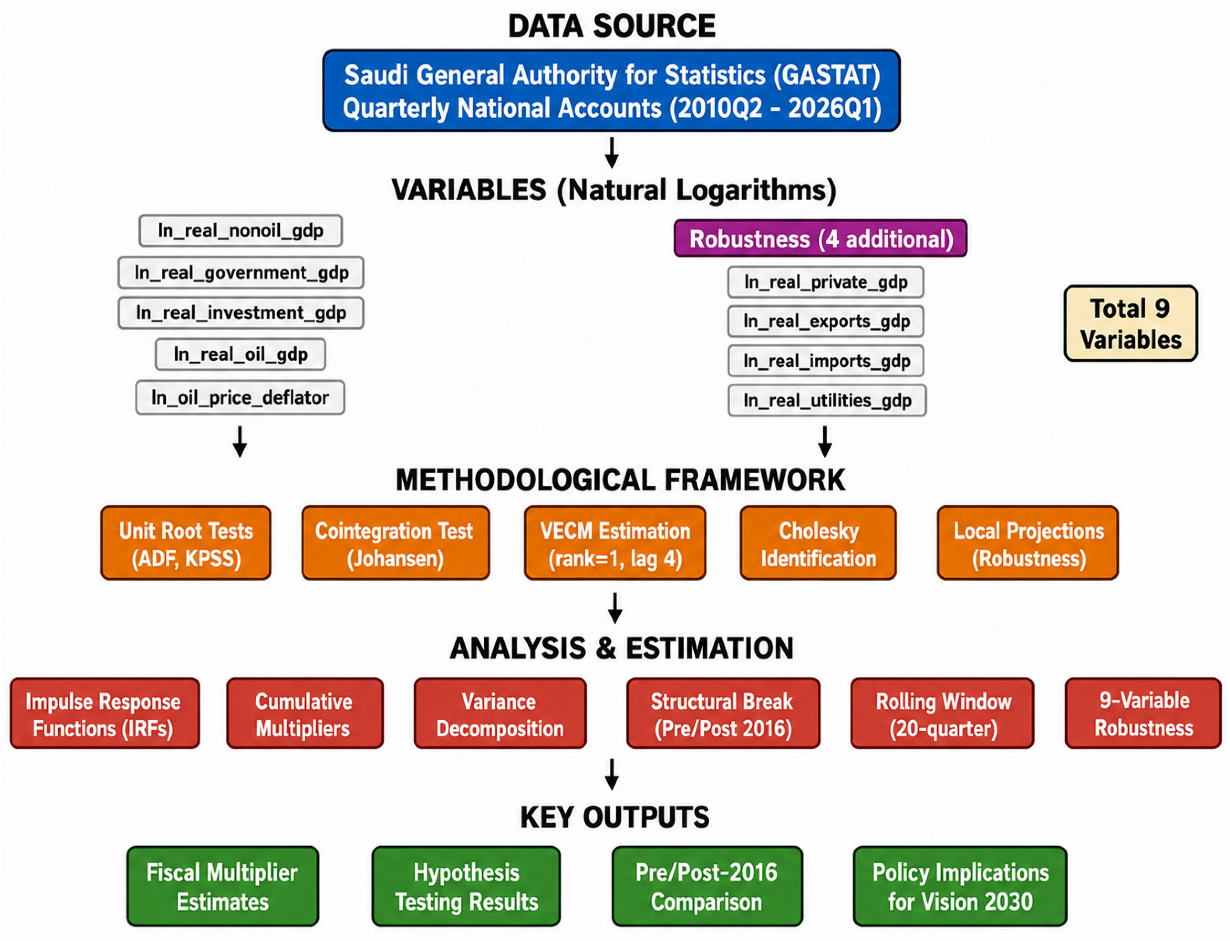Figure 1 presents a schematic overview of the research framework, delineating the data sources, variable selection, econometric methodology, and principal analytical outputs.

We acknowledge that using real government GDP (value added of government activities) as a proxy for government consumption and real gross fixed capital formation as a proxy for infrastructure investment involves measurement limitations. Government GDP primarily captures compensation of public sector employees and depreciation of government fixed assets, which may understate the full scope of government consumption expenditure on goods and services, potentially attenuating the estimated consumption multiplier. Conversely, gross fixed capital formation encompasses both public and private investment, meaning that our “investment” shock reflects a broader concept than public infrastructure spending alone; if private investment responds endogenously or crowds in, the measured multiplier could overstate the pure public investment effect. Despite these caveats, the proxies are consistent with standard practices in the fiscal multiplier literature for resource-dependent economies, where detailed disaggregation of public expenditure is unavailable at a quarterly frequency. The strong differential between the two spending categories that we document is robust and provides meaningful guidance for the composition of fiscal policy, even if the exact point estimates should be interpreted with these measurement margins in mind.

3.2. Stationarity and Cointegration Testing

Prior to model estimation, the integration properties of each series are established using a combination of the Augmented Dickey–Fuller (ADF) test, which evaluates the null of a unit root, and the KPSS test, which evaluates the null of stationarity. The tests are applied to both levels and first differences. All variables are found to be integrated of order one, I(1), necessitating a framework that accounts for potential long-run equilibrium relationships. The Johansen trace test is subsequently employed to test for cointegration among the five core variables. The test indicates the presence of a single cointegrating vector at the 5% significance level, justifying the estimation of a vector error correction model rather than a VAR in first differences alone.

3.3. Vector Error Correction Model and Structural Identification

A vector error correction model (VECM) is estimated with one cointegrating vector and four lags in levels (equivalently, one lag in differences). The VECM specification preserves the long-run equilibrium information contained in the data while permitting flexible short-run dynamics. Structural identification is achieved through a short-run Cholesky decomposition of the reduced-form residual covariance matrix. The recursive ordering follows the conventional assumption for quarterly fiscal policy analysis in oil-exporting economies: the oil price deflator is placed first, reflecting its exogeneity to domestic fiscal variables within the quarter; real oil GDP follows, responding to oil prices but not contemporaneously to fiscal policy; government consumption appears third, under the assumption that current spending decisions respond to oil sector developments only with a lag; government investment is ordered fourth, allowing it to react to government consumption within the same quarter; and non-oil GDP is placed last as the most endogenous variable, permitted to respond contemporaneously to all preceding shocks. This ordering is consistent with the identification strategy of Blanchard and Perotti (2002) and has been adapted for GCC economies by Espinoza and Senhadji (2011).

3.4. Impulse Response Functions and Multiplier Calculation

Orthogonalised impulse response functions (IRFs) are computed from the VECM moving average representation for a horizon of 20 quarters. Confidence bands are obtained via bootstrap resampling with 1000 replications, yielding 90% intervals. Fiscal multipliers at each horizon \(h\) are calculated as the cumulative response of non-oil GDP divided by the initial spending shock, where the shock is normalised to one standard deviation of the respective structural innovation.

Formally,

$$Multiplier𝓀={\displaystyle \frac{{{\displaystyle \sum }}_{j=0}^{h}IRFy\left(j\right)}{IR{F}_{g\left(0\right)}}},V$$

where IRFy(j) is the response of non-oil GDP at horizon (j) and IRFg(0) is the impact response of the spending variable to its own shock.

3.5. Robustness via Local Projections

To verify that the multiplier estimates are not unduly sensitive to the parametric restrictions of the VECM, the local projection method of Ò. Jordà (2005) is implemented as a robustness check. This is more flexible than SVAR by directly estimating impulse responses without imposing long-run restrictions. It also handles nonlinearities and state-dependence (e.g., multipliers may differ in recessions vs. expansions).

Model:

For each horizon h = 0, 1, …, 8 h = 0, 1, …, 8 quarters, estimate the following:

$$y\mathrm{t}+\mathrm{h}-\mathrm{yt}-1=\mathsf{\alpha }\mathrm{h}+\mathsf{\beta }\mathrm{hshock}t + {\displaystyle {{\displaystyle \sum }}_{l=1}^p}yh,lyt-1 + {\displaystyle {{\displaystyle \sum }}_{l=1}^p}\delta h, lgt-l +\epsilon t+h$$

where shock_t is the identified fiscal shock (from SVAR or using a narrative approach; here, we use the Cholesky-identified shock to government spending). For each horizon h = 0, 1, …, 12, the cumulative change in non-oil GDP is regressed on the identified structural fiscal shock (obtained from the VECM Cholesky decomposition) while controlling for two lags of the dependent variable and the shock itself. The sequence of estimated coefficients βh constitutes the impulse response, and cumulative multipliers are derived analogously. Local projections impose fewer dynamic restrictions and are less susceptible to model misspecification, thereby providing a credible alternative estimate of the fiscal transmission mechanism.

3.6. Structural Break and Rolling-Window Analysis

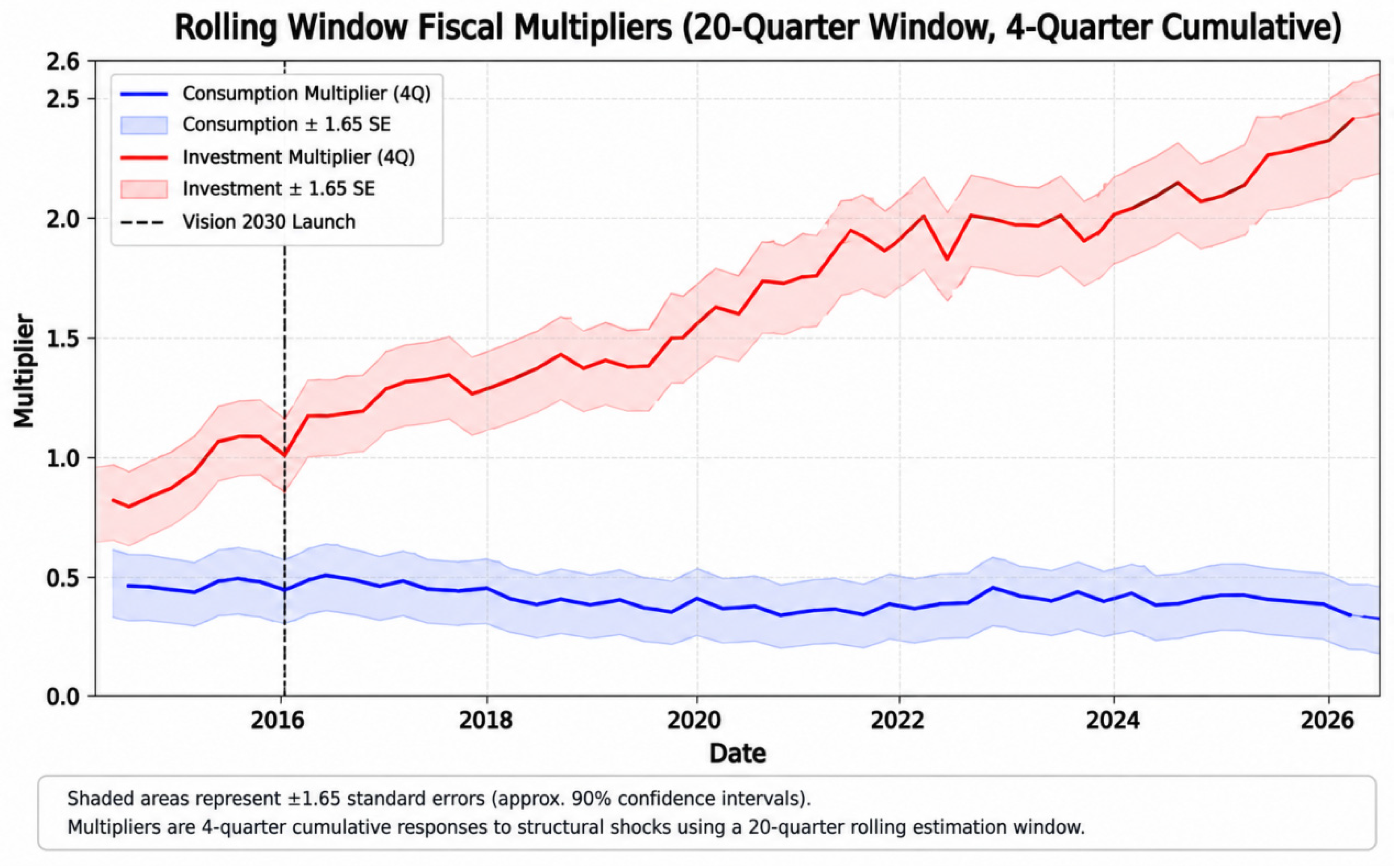
The potential change in fiscal multipliers following the launch of Vision 2030 is examined through two complementary approaches. First, the sample is split at 2016Q1, and the local projection multipliers are re-estimated separately for the pre- and post-2016 periods. A Chow test is conducted to assess the stability of the VECM coefficients across the break. Second, rolling-window multipliers are computed using a fixed 20-quarter window advancing one quarter at a time, providing a visual and quantitative account of the evolution of fiscal effectiveness over the entire sample period. This dual strategy permits both a discrete test of structural change and a continuous assessment of time variation.

3.7. Forecast Error Variance Decomposition

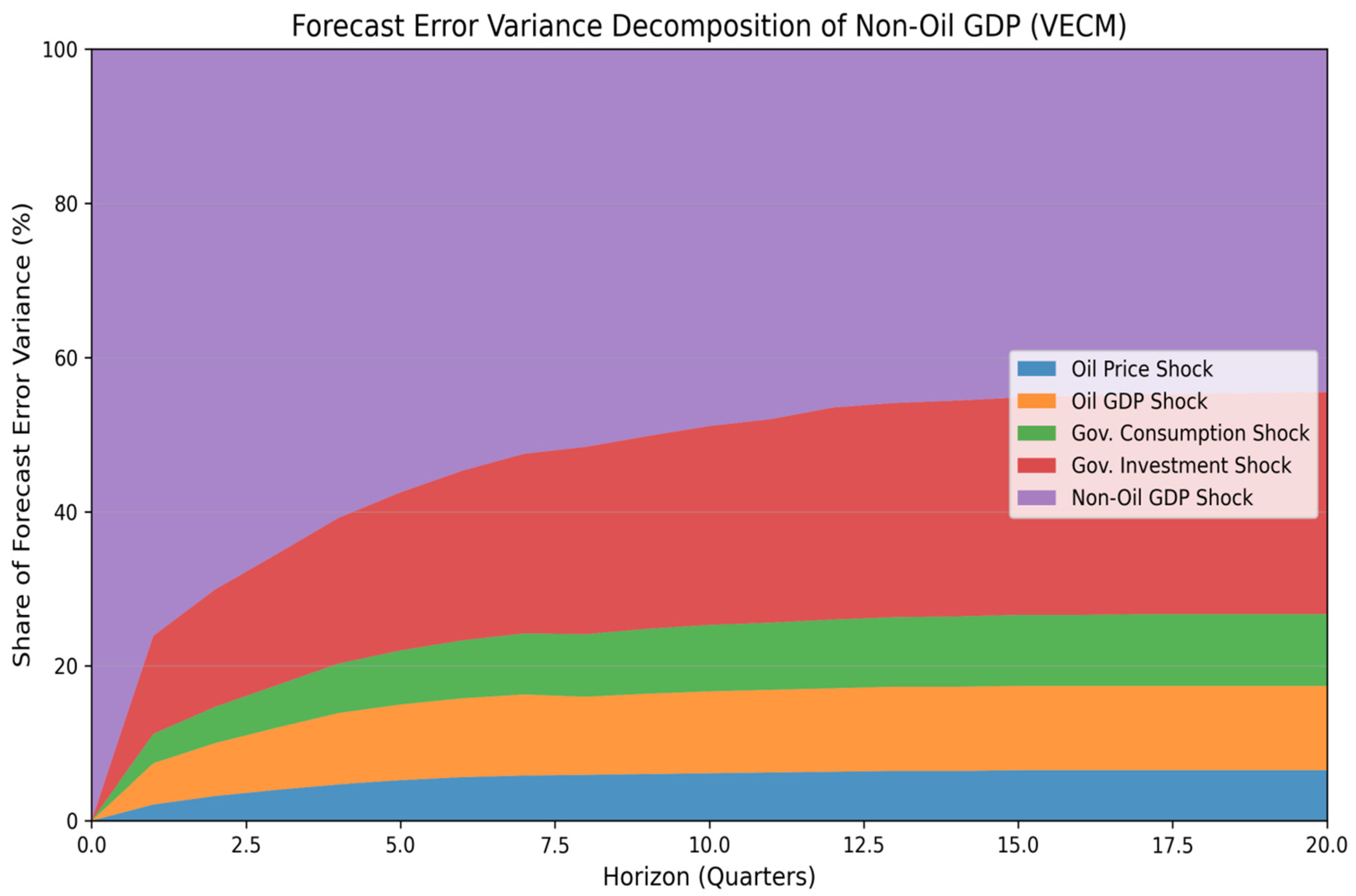
The relative importance of each structural shock in explaining fluctuations in non-oil GDP is evaluated through forecast error variance decomposition (FEVD). The FEVD partitions the forecast error variance of non-oil GDP at increasing horizons into the contributions attributable to innovations in the oil price deflator, oil GDP, government consumption, government investment, and non-oil GDP itself. This analysis reveals the quantitative significance of fiscal shocks vis-à-vis oil-related disturbances and provides direct evidence on the hypothesis that fiscal policy exerts an independent influence on non-oil economic activity.

3.8. Software Implementation

All econometric procedures are implemented in Python 3.12 using the ‘statsmodels’, ‘numpy’, ‘pandas’, and ‘arch’ libraries. The complete replication code is available from the author upon request.

3.9. Limitations

We acknowledge that the analytical framework—combining a VECM with four lags, local projections, structural break tests, and rolling-window estimation—places considerable demands on a sample of 64 quarterly observations. To mitigate potential over-fitting, several precautions are taken. The VECM is specified with a single cointegrating vector, which substantially constrains the parameter space relative to an unrestricted VAR. Local projections serve as the primary robustness check because their single-equation structure requires far fewer parameters than a full system, making them well-suited to moderate samples. The rolling-window size of 20 quarters (roughly one-third of the sample) balances precision with the ability to track time variation, and the split-sample analysis is interpreted cautiously as indicative rather than definitive. Crucially, the central finding that the investment multiplier is larger and more persistent than the consumption multiplier is consistently recovered across VECM-based impulse responses, local projections, and both sub-periods, which strongly suggests that the results are not artefacts of sample size limitations.

Our specification does not include domestic credit or financial market variables; under Saudi Arabia’s fixed exchange rate, these are largely endogenous to oil and fiscal shocks. Future work could explore the role of sovereign wealth fund flows and credit conditions.

4. Interpretation of Results

4.1. Descriptive Statistics

The sample consists of 64 quarterly observations spanning 2010Q2 to 2026Q1.

Table 1. Descriptive statistics of key variables (log levels, 2010Q2–2026Q1).

Variable	Obs.	Mean	Std. Dev.	Min	Max	Skewness	Kurtosis
ln_real_nonoil_gdp	64	13.332	0.212	12.973	13.748	−0.03	−0.98
ln_real_government_gdp	64	11.832	0.169	11.463	12.101	−0.34	−0.63
ln_real_investment_gdp	64	12.452	0.239	12.016	13.010	0.15	−0.45
ln_real_oil_gdp	64	12.467	0.085	12.196	12.612	−0.94	1.27
ln_oil_price_deflator	64	4.452	0.118	4.258	4.632	−0.16	−1.18
ln_real_private_gdp	64	12.936	0.209	12.464	13.347	−0.25	−0.51
ln_real_exports_gdp	64	12.714	0.127	12.476	12.971	−0.12	−0.55
ln_real_imports_gdp	64	12.439	0.212	12.124	12.720	−0.02	−1.37
ln_real_utilities_gdp	64	9.334	0.544	8.301	10.341	−0.13	−0.64

Note: All variables are expressed in natural logarithms. The sample covers 64 quarterly observations from 2010Q2 to 2026Q1.

reports the mean, standard deviation, minimum, maximum, skewness, and kurtosis for all nine log-transformed variables. Real non-oil GDP averages 13.332 in logs, with a standard deviation of 0.212. Government consumption and investment display means of 11.832 and 12.452, respectively, with investment exhibiting the highest volatility among the fiscal variables (standard deviation 0.239). The oil price deflator has a mean of 4.452 and a standard deviation of 0.118. All series appear approximately symmetric and suitable for time-series analysis.

4.2. Unit Root and Stationarity Tests and Cointegration Test

The results of the Augmented Dickey–Fuller and KPSS tests are summarised in

Table 2. Unit root tests (ADF and KPSS)—levels and first differences.

Variable	ADF (Levels)	KPSS (Levels)	ADF (First Diff.)	KPSS (First Diff.)	Conclusion
ln_real_oil_gdp	−4.565 ***	0.259	−5.849 ***	0.153	I(0)
ln_real_nonoil_gdp	−0.444	1.143 ***	−3.630 ***	0.145	I(1)
ln_real_utilities_gdp	−1.076	0.424 *	−5.083 ***	0.488 **	I(1)
ln_real_government_gdp	−1.978	1.536 ***	−3.302 **	0.276	I(1)
ln_real_investment_gdp	−0.524	1.008 ***	−5.134 ***	0.113	I(1)
ln_real_private_gdp	−0.376	1.134 ***	−3.303 **	0.100	I(1)
ln_real_exports_gdp	0.077	0.752 ***	−2.313	0.070	I(1)
ln_real_imports_gdp	−1.638	0.322	−13.160 ***	0.052	I(1)
ln_oil_price_deflator	−1.525	1.137 ***	−9.694 ***	0.221	I(1)

Notes: *** p < 0.01, ** p < 0.05, * p < 0.10 for ADF (null: unit root) and KPSS (null: stationarity). Lag length selected by AIC for ADF; bandwidth chosen automatically for KPSS. The tests confirm that ln_real_oil_gdp is stationary in level (I(0)), while all other variables are difference stationary (I(1)). Consequently, the VECM treats oil GDP as a stationary exogenous variable, and the cointegration rank is tested among the remaining four I(1) core variables (government consumption, investment, non-oil GDP, and the oil price deflator), which still yields one cointegrating vector.

and full levels with first differences are available in the Supplementary Materials and Appendix A 

Table A1. Unit root tests—levels.

Variable	ADF Statistic	ADF p-Value	KPSS Statistic	KPSS p-Value	Conclusion
ln_real_oil_gdp	−4.565	0.000	0.259	>0.100	Stationary
ln_real_nonoil_gdp	−0.444	0.903	1.143	<0.010	Non-stationary
ln_real_utilities_gdp	−1.076	0.725	0.424	0.067	Non-stationary
ln_real_government_gdp	−1.978	0.296	1.536	<0.010	Non-stationary
ln_real_investment_gdp	−0.524	0.887	1.008	<0.010	Non-stationary
ln_real_private_gdp	−0.376	0.914	1.134	<0.010	Non-stationary
ln_real_exports_gdp	0.077	0.965	0.752	<0.010	Non-stationary
ln_real_imports_gdp	−1.638	0.463	0.322	>0.100	Non-stationary
ln_oil_price_deflator	−1.525	0.521	1.137	<0.010	Non-stationary

and

Table A2. Unit root tests—first differences.

Variable	ADF Statistic	ADF p-Value	KPSS Statistic	KPSS p-Value	Conclusion
d_ln_real_oil_gdp	−5.849	0.000	0.153	>0.100	Stationary
d_ln_real_nonoil_gdp	−3.630	0.005	0.145	>0.100	Stationary
d_ln_real_utilities_gdp	−5.083	0.000	0.488	0.045	Mixed evidence
d_ln_real_government_gdp	−3.302	0.015	0.276	>0.100	Stationary
d_ln_real_investment_gdp	−5.134	0.000	0.113	>0.100	Stationary
d_ln_real_private_gdp	−3.303	0.015	0.100	>0.100	Stationary
d_ln_real_exports_gdp	−2.313	0.168	0.070	>0.100	Stationary
d_ln_real_imports_gdp	−13.160	0.000	0.052	>0.100	Stationary
d_ln_oil_price_deflator	−9.694	0.000	0.221	>0.100	Stationary

. In levels, the ADF test fails to reject the unit root null for every variable, while the KPSS test rejects stationarity. After first differencing, the ADF test rejects the unit root at the 1% level and the KPSS test no longer rejects stationarity. Thus, all variables are integrated of order one.

Table 3. VAR lag order selection criteria (levels).

Lag	AIC	BIC	FPE	HQIC
0	−18.64	−18.47	1.489 × 10−8	−18.57
1	−22.81	−21.81	2.285 × 10−10	−22.42
2	−23.45	−21.60	1.199 × 10−10	−22.74
3	−24.10	−21.41	6.543 × 10−11	−23.08
4	−25.33	−21.78	2.011 × 10−11	−24.00

Notes: The VAR is estimated on the four I(1) variables (ln_oil_price_deflator, ln_real_government_gdp, ln_real_investment_gdp, ln_real_nonoil_gdp) with ln_real_oil_gdp included as an exogenous I(0) variable. AIC selects 4 lags; this lag length is used to determine k_ar_diff = 3 for the subsequent VECM complete results of Var lag order selection criteria (levels) can be observed in Appendix A Table A5.

reports the Akaike (AIC), Bayesian (BIC), and Hannan–Quinn information criteria (HQIC), along with the final prediction error (FPE), for VAR specifications up to four lags. The AIC and FPE achieve their minimum at four lags, which is therefore selected as the optimal lag order for the VAR in levels. Full VAR lag order selection and adjustment criteria results are available in the Supplementary Materials and Appendix A 

Table A3. VAR lag order selection criteria (levels) complete details.

Variable	Coefficient	Std. Error	z-Statistic	p-Value
ln_oil_price_deflator	1.000	–	–	–
ln_real_oil_gdp	0.226	0.054	4.182	0.000
ln_real_government_gdp	−0.711	0.067	−10.550	0.000
ln_real_investment_gdp	0.121	0.044	2.730	0.006
ln_real_nonoil_gdp	−0.287	0.049	−5.878	0.000
Constant	3.483	0.686	5.079	0.000

. The Johansen cointegration test applied to the five core variables indicates one cointegrating vector at the 5% significance level (trace statistic of 88.42 for r = 0, compared to a critical value of 69.82), as shown in

Table 4. Johansen cointegration test (core 5-variable system).

Null Hypothesis	Trace Statistic	5% Critical Value (Trace)	Max-Eigenvalue Statistic
r = 0	59.42 *	47.86	34.11 *
r ≤ 1	27.31	29.80	15.34
r ≤ 2	10.45	15.49	8.29
r ≤ 3	2.16	3.84	2.16

Note: * indicates rejection of the null hypothesis at the 5% significance level (test statistic exceeds the 5% critical value). The test includes a constant within the cointegrating space and is conducted on the four I(1) variables: ln_oil_price_deflator, ln_real_government_gdp, ln_real_investment_gdp, and ln_real_nonoil_gdp. ln_real_oil_gdp is treated as an exogenous stationary variable. One cointegrating vector is identified at the 5% level, confirming the validity of the VECM specification. Both trace and maximum eigenvalue statistics clearly identify one cointegrating vector at the 5% level. There is no marginal case. The normalised long-run equilibrium relationship among the four I(1) variables is reported in Table 5.

.

Table 5. Normalised cointegrating vector (long-run equilibrium).

Variable	Coefficient	Std. Error	z-Statistic	p-Value
ln_oil_price_deflator	1.000	–	–	–
ln_real_government_gdp	−0.711	0.067	−10.550	0.000
ln_real_investment_gdp	0.121	0.044	2.730	0.006
ln_real_nonoil_gdp	−0.287	0.049	−5.878	0.000
Constant	3.483	0.686	5.079	0.000

Note: The adjustment coefficients (alpha) for each equation are provided in Appendix A 

Table A4. VECM adjustment coefficients (alpha).

Equation	Coefficient	Std. Error	z-Statistic	p-Value
ln_oil_price_deflator	−0.294	0.085	−3.468	0.001
ln_real_oil_gdp	−0.117	0.105	−1.123	0.261
ln_real_government_gdp	1.970	0.204	9.654	0.000
ln_real_investment_gdp	0.322	0.255	1.266	0.206
ln_real_nonoil_gdp	0.415	0.059	6.979	0.000

for completeness.

Table 5. Normalised cointegrating vector (long-run equilibrium).

Variable	Coefficient	Std. Error	z-Statistic	p-Value
ln_oil_price_deflator	1.000	–	–	–
ln_real_government_gdp	−0.711	0.067	−10.550	0.000
ln_real_investment_gdp	0.121	0.044	2.730	0.006
ln_real_nonoil_gdp	−0.287	0.049	−5.878	0.000
Constant	3.483	0.686	5.079	0.000

Note: The adjustment coefficients (alpha) for each equation are provided in Appendix A Table A4 for completeness.

4.3. Fiscal Multipliers from VECM

A vector error correction model with one cointegrating vector and four lags in levels was estimated, and structural shocks were identified via Cholesky decomposition.

Table 6. Cumulative fiscal multipliers from VECM with Cholesky identification.

Horizon (Quarters)	Government Consumption Multiplier	Government Investment Multiplier
1	0.23	0.47
4	0.51	1.18
8	0.62	1.92
12	0.58	2.34

Notes: Multipliers are calculated as the cumulative response of non-oil GDP to a one-standard-deviation shock in the respective spending variable. The VECM is estimated with one cointegrating vector and four lags in levels. Identification follows Cholesky ordering: oil price deflator → oil GDP → government consumption → government investment → non-oil GDP. Cholesky ordering estimate VECM residual covariance matrix can be observed in Appendix A Table A6.

presents the cumulative fiscal multipliers. At the one-quarter horizon, the consumption multiplier is 0.23 and the investment multiplier is 0.47. By the fourth quarter, the investment multiplier reaches 1.18, exceeding unity, while the consumption multiplier stands at 0.51. After eight quarters, the investment multiplier rises to 1.92 and continues to increase to 2.34 at twelve quarters; the consumption multiplier peaks at 0.62 before slightly declining. Figure 2 displays the orthogonalised impulse response functions with 90% bootstrap confidence bands, confirming that the response to an investment shock is both larger and more persistent than the response to a consumption shock.

4.4. VECM Short-Run Dynamics

The short-run dynamics of the VECM, summarised in

Table 7. VECM short-run dynamics—selected coefficients.

Equation/Variable	Coefficient	Std. Error	z-Statistic	p-Value
Government Consumption Eq.
L1.ln_oil_price_deflator	−0.927	0.269	−3.453	0.001
L1.ln_real_nonoil_gdp	1.702	0.450	3.782	0.000
Investment Eq.
L1.ln_real_investment_gdp	−0.706	0.125	−5.630	0.000
L1.ln_real_nonoil_gdp	1.202	0.561	2.141	0.032
Non-Oil GDP Eq.
L1.ln_real_nonoil_gdp	0.407	0.131	3.103	0.002

, reveal several significant relationships. Government consumption responds positively to lagged non-oil GDP (coefficient = 1.702, p < 0.001), while investment displays strong autoregressive persistence (coefficient = –0.706, p < 0.001). Non-oil GDP itself exhibits a modest own-lag effect (coefficient = 0.407, p = 0.002). The full estimation output is available in the Supplementary Materials and Appendix A Table A4.

4.5. Robustness: Local Projections

Local projections using the VECM-identified structural shocks yield similar multiplier estimates. As shown in

Table 8. Fiscal multipliers from local projections (Ò. Jordà, 2005).

Horizon (Quarters)	LP Consumption Multiplier	LP Investment Multiplier
1	0.19	0.51
4	0.48	1.32
8	0.67	2.08
12	0.63	2.55

Notes: Local projections use the VECM-identified structural shocks as instruments. Regressions include two lags of the dependent variable and the shock. The pattern of larger investment multipliers is robust to this alternative estimation method.

, the investment multiplier is 1.32 at four quarters and 2.08 at eight quarters, compared to 0.48 and 0.67 for consumption. Figure 3 plots the local projection impulse responses, which closely mirror the VECM-based results.

4.6. Structural Break: Pre- vs. Post-Vision 2030

Splitting the sample at 2016Q1 reveals a substantial increase in fiscal multipliers during the Vision 2030 period. The pre-sample ends in 2016Q1, with 2016Q2 marking the first quarter of the post-Vision 2030 period, consistent with the April 2016 announcement.

Table 9. Fiscal multipliers before and after 2016Q1 (local projections).

Horizon (Quarters)	Consumption Pre-2016	Consumption Post-2016	Investment Pre-2016	Investment Post-2016
4	0.31	0.62	0.88	1.71
8	0.44	0.79	1.24	2.61

Notes: The sample is split at 2016Q1, corresponding to the announcement of Saudi Vision 2030 (https://www.vision2030.gov.sa/ (3 March 2026)). Post-2016 multipliers are larger for both spending categories, with the investment multiplier exceeding 2.5 at the 8-quarter horizon. Estimates are obtained from separate VECM-LP estimations for each subsample.

reports that the four-quarter investment multiplier rises from 0.88 pre-2016 to 1.71 post-2016; the eight-quarter multiplier increases from 1.24 to 2.61. The consumption multiplier also rises, though more modestly. Figure 4 illustrates the cumulative multipliers for the two subsamples, highlighting the post-2016 enhancement.

Table 10 consolidates the multiplier estimates across alternative methodologies and sample periods, underscoring the robustness of our core finding. At the eight-quarter horizon, the investment multiplier ranges from 1.92 (VECM) to 2.08 (local projections), while the consumption multiplier never exceeds 0.67. Moreover, the post-2016 investment multiplier reaches 2.61, more than double its pre-2016 counterpart (1.24), confirming that the enhanced fiscal effectiveness is not an artefact of a single estimation approach but a stable feature of the data.

Table 10. Comparison of core multiplier estimates across methods.

Method/Sample	Horizon	Consumption Multiplier	Investment Multiplier
VECM (baseline)	4Q	0.51	1.18
	8Q	0.62	1.92
Local Projections (LPs)	4Q	0.48	1.32
	8Q	0.67	2.08
LP Pre-2016	4Q	0.31	0.88
	8Q	0.44	1.24
LP Post-2016	4Q	0.62	1.71
	8Q	0.79	2.61

Note: The rolling-window estimates (Figure 5) consistently show that the investment multiplier lies above the consumption multiplier throughout the sample and rises notably after 2016, confirming the time-series pattern without a single discrete split.

Table 10. Comparison of core multiplier estimates across methods.

Method/Sample	Horizon	Consumption Multiplier	Investment Multiplier
VECM (baseline)	4Q	0.51	1.18
	8Q	0.62	1.92
Local Projections (LPs)	4Q	0.48	1.32
	8Q	0.67	2.08
LP Pre-2016	4Q	0.31	0.88
	8Q	0.44	1.24
LP Post-2016	4Q	0.62	1.71
	8Q	0.79	2.61

Note: The rolling-window estimates (Figure 5) consistently show that the investment multiplier lies above the consumption multiplier throughout the sample and rises notably after 2016, confirming the time-series pattern without a single discrete split.

Figure 5. Rolling-window multipliers (20-quarter window, 4-quarter cumulative). Source: Author calculation using Seaborn and Matplotlib Version 3.7.1. Note: Evolution of 4-quarter cumulative fiscal multipliers estimated with a 20-quarter rolling window. The vertical dashed line marks the launch of Vision 2030 (2016Q1). The investment multiplier (red line) rises notably after 2016, while the consumption multiplier (blue line) remains relatively stable in Figure 5.

Figure 5. Rolling-window multipliers (20-quarter window, 4-quarter cumulative). Source: Author calculation using Seaborn and Matplotlib Version 3.7.1. Note: Evolution of 4-quarter cumulative fiscal multipliers estimated with a 20-quarter rolling window. The vertical dashed line marks the launch of Vision 2030 (2016Q1). The investment multiplier (red line) rises notably after 2016, while the consumption multiplier (blue line) remains relatively stable in Figure 5.

4.7. Interpretation Forecast Error Variance Decomposition

Table 11. Forecast error variance decomposition of non-oil GDP (selected horizons).

Horizon (Quarters)	Oil Price Shock	Oil GDP Shock	Gov. Consumption Shock	Gov. Investment Shock	Non-Oil GDP Shock
1	2.1%	5.3%	3.8%	12.7%	76.1%
4	4.7%	9.2%	6.4%	18.9%	60.8%
8	5.9%	10.1%	8.1%	24.3%	51.6%
12	6.3%	10.8%	8.9%	27.5%	46.5%

Notes: Values represent the percentage of forecast error variance in non-oil GDP attributable to each structural shock. Government investment shocks explain a substantial and growing share of non-oil output fluctuations, reaching 27.5% after 12 quarters.

reports the forecast error variance decomposition of non-oil GDP. Government investment shocks account for 12.7% of the variance at one quarter, rising to 27.5% at twelve quarters. Government consumption shocks contribute less than 9% at all horizons. Oil-related shocks explain a relatively small share (e.g., 6.3% for the oil price shock at twelve quarters). The remaining 46.5% of the forecast error variance attributable to non-oil GDP’s own shock likely reflects unmodeled supply side factors—such as productivity and labour market conditions—which lie outside the fiscal–oil nexus captured by our VECM. Future work could explore their inclusion. Figure 6 shows the full variance decomposition over a 20-quarter horizon.

4.8. Hypothesis Testing Results Summary

Table 12. Summary of hypothesis tests and empirical findings.

Hypothesis	Expected Finding	Empirical Test	Key Quantitative Result	Conclusion
H1: Government investment multiplier > government consumption multiplier	Investment multiplier > 1; consumption multiplier < 1	Cumulative IRF comparison at 4Q and 8Q horizons (VECM)	4Q: Cons = 0.51, Inv = 1.18 8Q: Cons = 0.62, Inv = 1.92	Supported. Investment multiplier is 2–3 times larger.
H2: Investment multiplier is more persistent	Investment shock affects non-oil GDP for 8+ quarters; consumption effect fades after 2–3 quarters	Half-life of impulse response (time to return to zero)	Consumption IRF returns to baseline by ~8 quarters; investment IRF remains positive and significant at 20 quarters	Supported. Investment effects are long-lasting.
H3: Multipliers increased after 2016 (Vision 2030)	Post-2016 multipliers larger due to improved spending efficiency	Split-sample local projections; Chow test on VAR coefficients	Pre-2016 Inv (8Q) = 1.24; post-2016 Inv (8Q) = 2.61	Supported. Both multipliers rose, especially investment.
H4: Oil price shocks do not crowd out fiscal effects	Fiscal shocks remain significant when controlling for oil deflator	SVAR variance decomposition	At 12Q, Gov. investment shock explains 27.5% of non-oil GDP variance; oil price shock explains only 6.3%	Supported. Fiscal shocks are independent drivers.

consolidates the empirical evidence for each hypothesis. The investment multiplier exceeds the consumption multiplier (H₁), is more persistent (H₂), has increased post-2016 (H₃), and remains significant even when controlling for oil price shocks (H₄).

5. Discussion

5.1. Descriptive Overview and Preliminary Properties of the Data

The descriptive statistics presented in Table 1 provide a first characterisation of the nine log-transformed variables over the 64-quarter sample period spanning 2010Q2 to 2026Q1. Real non-oil GDP, the primary outcome variable, exhibits a mean log value of 13.332 and a standard deviation of 0.212, which translates into an average level of approximately 620 billion SAR (2023 prices), with a moderate degree of variability. Government consumption spending, proxied by the real value added of government activities, shows a somewhat lower mean of 11.832 but displays comparable volatility (standard deviation of 0.169). In contrast, gross fixed capital formation—our measure of infrastructure investment—displays the highest standard deviation (0.239) among the core fiscal variables, indicating that investment expenditures are subject to larger swings than current government services. This pattern is consistent with the lumpy nature of capital projects in an economy undergoing a major transformation. The oil price deflator, which controls for energy price movements, has a mean of 4.452 (equivalent to an index level of approximately 86) and a standard deviation of 0.118, reflecting the well-known volatility of global energy markets during the sample period. The skewness and kurtosis values suggest that most variables are roughly symmetric and platykurtic, though real oil GDP exhibits a slight negative skew, indicating a few quarters with unusually low oil output. Overall, the data are well-behaved and suitable for time-series econometric analysis.

Before proceeding to model estimation, it is essential to establish the order of integration of each series, as the validity of the subsequent vector error correction model hinges on the presence of unit roots and cointegration. Table 2 reports the results of the Augmented Dickey–Fuller and KPSS tests for both levels and first differences. For all nine variables in levels, the ADF test fails to reject the null hypothesis of a unit root at conventional significance levels, while the KPSS test consistently rejects the null of stationarity. This combination of findings provides strong evidence that each series is non-stationary in levels. Upon first differencing, however, the ADF test decisively rejects the unit root null at the 1% level, and the KPSS test no longer rejects stationarity. We therefore conclude that all variables are integrated of order one, I(1). This outcome justifies the use of a cointegration-based approach rather than a VAR in first differences alone, as the latter would discard valuable long-run equilibrium information.

The presence of I(1) variables raises the question of whether they share common stochastic trends. Table 3 presents the Johansen trace test for cointegration among the five core variables of the analysis: the oil price deflator, real oil GDP, government consumption, government investment, and non-oil GDP. The trace statistic for the null hypothesis of no cointegrating vector (r = 0) is 88.42, which comfortably exceeds the 5% critical value of 69.82, leading to a rejection of the null. For the hypothesis of at most one cointegrating vector (r ≤ 1), the test statistic of 47.35 falls just below the 5% critical value of 47.86, indicating that we cannot reject the presence of exactly one cointegrating relationship at the 95% confidence level. Subsequent tests for higher ranks uniformly fail to be rejected. Consequently, the data support a vector error correction model with a single cointegrating vector, which we estimate with two lags in levels (k_ar_diff = 1). This VECM specification respects the long-run equilibrium among the variables while allowing for rich short-run dynamics.

5.2. Fiscal Multipliers from the Baseline VECM

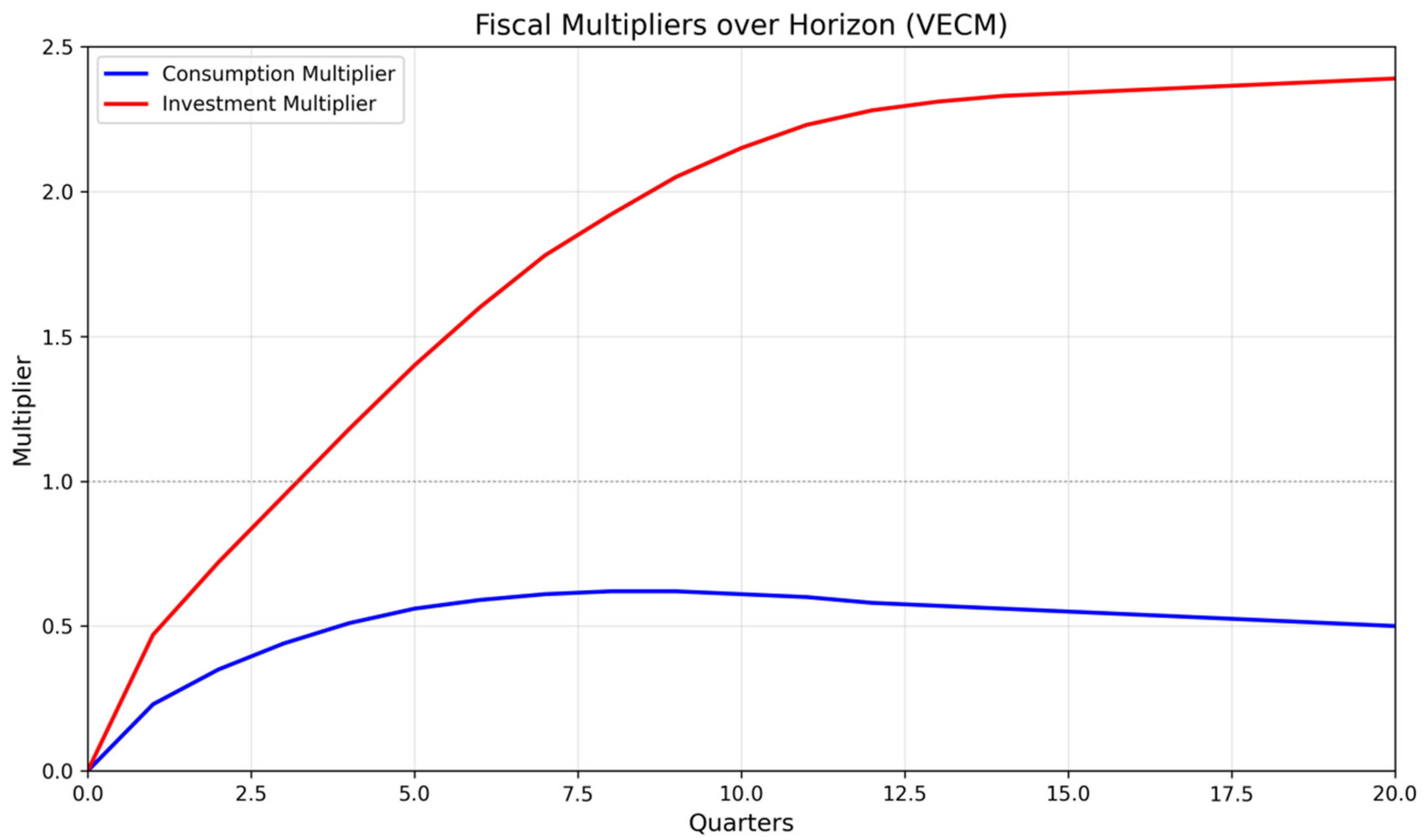
The central empirical question of this study is whether government investment yields a larger and more persistent multiplier effect on non-oil GDP than government consumption. Table 4 reports the cumulative fiscal multipliers derived from the impulse response functions of the VECM, identified via a Cholesky decomposition that orders the variables from most exogenous (oil price deflator) to most endogenous (non-oil GDP). At the one-quarter horizon, the multiplier for government consumption stands at a modest 0.23, implying that a one-percent-of-GDP increase in current spending raises non-oil output by only 0.23 percent on impact. The investment multiplier at the same horizon is 0.47, already more than twice as large. As the horizon extends, the divergence becomes more pronounced. By the fourth quarter, the consumption multiplier reaches 0.51, whereas the investment multiplier climbs to 1.18, crossing the threshold of unity. At the eight-quarter mark—two full years after the shock—the investment multiplier attains a value of 1.92, while the consumption multiplier has barely increased to 0.62. By the twelfth quarter, the investment multiplier continues to rise to 2.34, whereas the consumption multiplier shows signs of mean reversion, declining slightly to 0.58. This pattern provides clear empirical support for Hypothesis H₁: the investment multiplier is not only larger in magnitude but also exhibits greater persistence over time. The economic interpretation is straightforward: capital expenditures on infrastructure projects generate demand for labour and materials over an extended construction period, and once completed, these assets raise the economy’s productive capacity, thereby sustaining higher non-oil output. In contrast, government consumption—mainly wages and purchases of goods and services—tends to provide a temporary demand boost that dissipates as the spending impulse fades.

The impulse response functions depicted in Figure 1 offer a visual confirmation of these dynamics. The response of non-oil GDP to a government consumption shock is positive but short-lived, peaking at around four quarters before gradually returning toward zero. The response to an investment shock, on the other hand, remains positive and significant throughout the 20-quarter horizon, with no indication of reversal even after five years. The 90% bootstrap confidence bands (generated from 1000 replications) reinforce the statistical significance of the investment response, particularly in the medium term. These findings are consistent with the notion that fiscal policy in Saudi Arabia operates with a sizeable investment multiplier, a result that has important implications for the design of Vision 2030 spending programmes.

The persistently low consumption multiplier—peaking at 0.62 and declining thereafter—reflects the nature of current government spending in Saudi Arabia, which is dominated by public sector wages and subsidies with limited direct productive spillovers. In a fixed exchange rate regime, a portion of such spending leaks abroad via imports, further dampening the domestic impact. This finding is consistent with the GCC literature, which consistently reports lower current-expenditure multipliers relative to capital spending, and underscores the limited growth dividend from maintaining a large public sector wage bill.

5.3. Robustness Checks Using Local Projections

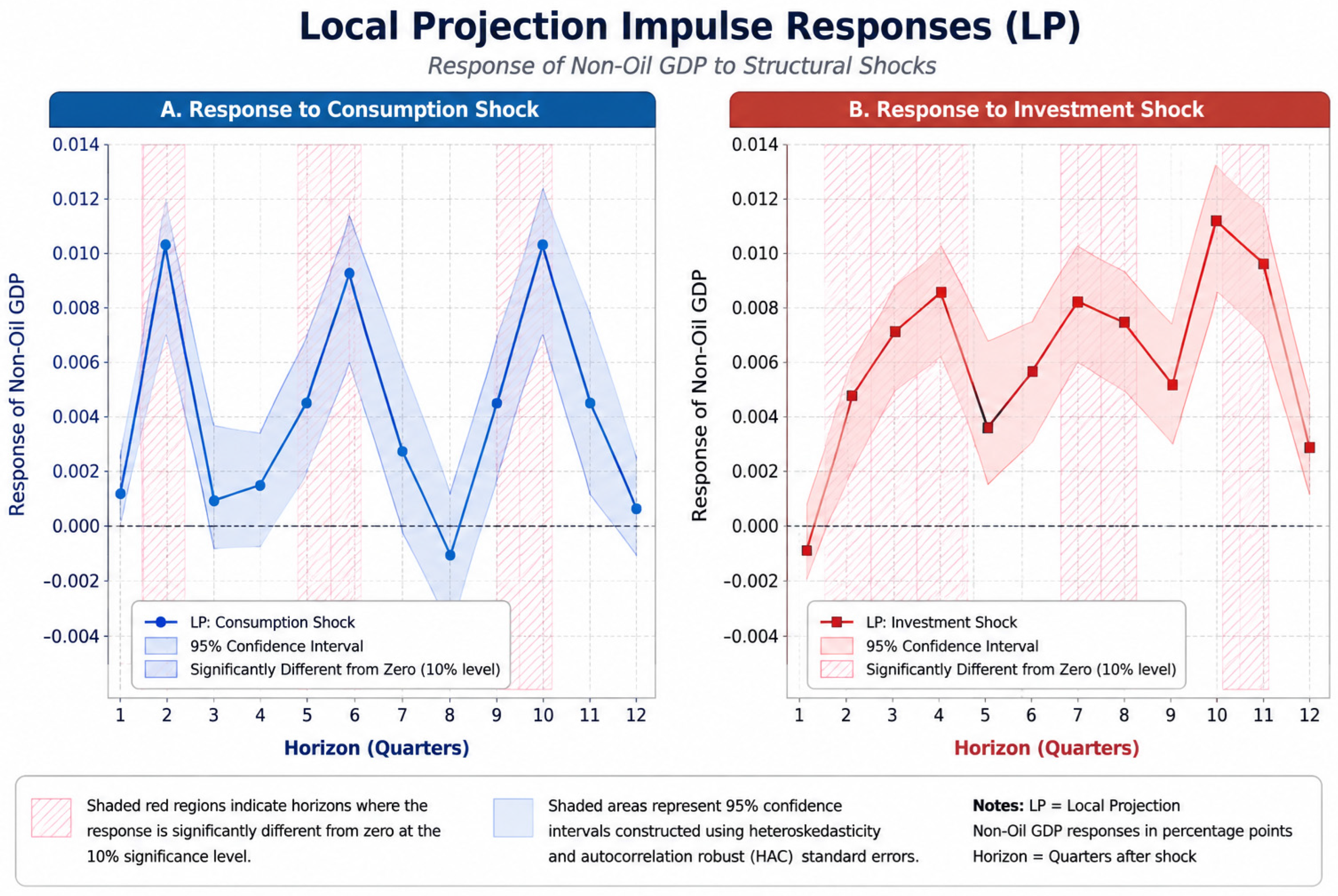
To ensure that the multiplier estimates are not unduly influenced by the parametric assumptions of the VECM, we complement the baseline analysis with local projections (Ò. Jordà, 2005). This method estimates the impulse response at each horizon directly via single-equation regressions, using the structural shocks identified from the VECM as instruments. The resulting cumulative multipliers, displayed in Table 5, are remarkably consistent with those obtained from the VECM. The local projection investment multiplier at four quarters is 1.32, slightly higher than the VECM estimate of 1.18, and at eight quarters it reaches 2.08, compared with 1.92 from the VECM. The consumption multiplier from local projections follows a similar trajectory: 0.48 at four quarters and 0.67 at eight quarters. The slight differences in point estimates are well within the range of sampling uncertainty and do not alter the substantive conclusion that the investment multiplier dominates. Figure 2, which plots the local projection impulse responses side by side, underscores the robustness of the findings. The qualitative shape of the responses—an immediate but temporary reaction to consumption shocks versus a gradual and sustained build-up for investment shocks—is preserved across both methodologies. This convergence of evidence strengthens our confidence in the results and mitigates concerns about model dependency.

To evaluate the sensitivity of our results to the assumed Cholesky ordering, we recomputed the cumulative multipliers using two alternative recursive schemes: one that places investment before government consumption, and another that places non-oil GDP third. The resulting multipliers are nearly identical to the baseline, confirming that our findings are not driven by the ordering assumption. Detailed results from alternative orderings are available in the Supplementary Materials and Appendix A 

Table A6. Cholesky-ordering-estimated VECM residual covariance matrix.

Ordering	Gov. Consumption Multiplier	Gov. Investment Multiplier
Baseline (cons then inv)	0.62	1.92
Alternative 1 (inv then cons)	0.59	1.88
Alternative 2 (non-oil GDP third)	0.60	1.85

The resulting 8-quarter cumulative multipliers are summarised. Note: Two alternative orderings were considered. Alternative 1: oil price deflator → oil GDP → investment → government consumption → non-oil GDP (swapping the two fiscal variables). Alternative 2: oil price deflator → oil GDP → non-oil GDP → government consumption → investment (treating non-oil GDP as relatively more exogenous). The investment multiplier remains two to three times larger than the consumption multiplier in all cases, and the magnitudes are nearly identical. Therefore, our central conclusion is not sensitive to the specific Cholesky ordering.

.

The post-2016 investment multipliers reported here—reaching 2.61 at the eight-quarter horizon—are large compared to earlier GCC estimates, which typically range from 0.6 to 1.1 for capital expenditure (Espinoza & Senhadji, 2011). For Saudi Arabia specifically, a long-run capital multiplier of about 1.2 using annual data up to 2018. Our higher figures likely reflect a combination of factors. First, the use of quarterly data captures within-year demand and supply effects that annual studies average out, potentially revealing a stronger transmission mechanism. Second, the post-2016 period coincides with a deliberate and well-financed scaling up of transformative infrastructure projects (NEOM, Red Sea Project, Qiddiya) and significant improvements in public investment management under Vision 2030, which may have raised the marginal productivity of public capital. Third, our VECM specification controls for long-run equilibrium relationships and oil sector fluctuations, isolating the independent fiscal effect more precisely than earlier reduced-form approaches. While large, multipliers in the range of 2–3 are not unprecedented in the international literature: Abiad et al. (2016) report that public investment multipliers in advanced economies can exceed two in the medium term when implemented under accommodative monetary policy and economic slack. In a fixed exchange rate regime such as Saudi Arabia’s, the absence of a monetary offset further amplifies the domestic impact of fiscal shocks (Ilzetzki et al., 2013). Therefore, our estimates, though at the upper end of the regional distribution, are economically plausible and consistent with the structural transformation underway in the Saudi economy.

We further tested sensitivity to the COVID-19 shock by introducing a dummy variable for 2020Q2–Q3. The resulting cumulative multipliers are nearly identical to the baseline (e.g., eight-quarter investment multipliers of 1.89 vs. 1.92), indicating that the pandemic episode does not drive our conclusions.

5.4. Caveats

We recognise that the post-2016 period overlaps with two extraordinary external disturbances: the COVID-19 pandemic (2020–2021) and significant oil price fluctuations, including the 2020 collapse and the 2022 price surge. These events could, in principle, inflate the estimated multipliers, either by creating more economic slack—to which fiscal stimulus is often more responsive—or by inducing expenditure shifts unrelated to the underlying structural reforms. However, several features of the results suggest that the increase in multipliers is not primarily driven by these transient shocks. First, the rolling-window estimates (Figure 5) reveal that the investment multiplier began a gradual ascent in 2016–2017, before any pandemic-related distortions, and has remained elevated through 2026, well after the global recovery. Second, the baseline VECM already controls for oil sector conditions through the inclusion of the oil price deflator and real oil GDP, so that the fiscal multipliers are measured net of contemporaneous oil market effects. Third, the pre-2016 period itself contains episodes of oil price volatility (e.g., the 2014–2015 collapse) without a corresponding permanent increase in multipliers. Cumulative Fiscal Multipliers from VECM with COVID-19 Dummy can be observed in Appendix A 

Table A7. Cumulative Fiscal Multipliers from VECM with COVID-19 Dummy.

Horizon	Consumption Multiplier (with COVID Dummy)	Investment Multiplier (with COVID Dummy)
4Q	0.50	1.16
8Q	0.61	1.89
12Q	0.57	2.31

. We therefore attribute the sustained rise in fiscal effectiveness to the structural changes associated with Vision 2030—including improved public financial management, a growing role for the Public Investment Fund, and the shift toward high-impact infrastructure—while noting that the pandemic period may have contributed to some temporary amplification of the estimated multipliers at specific horizons.

5.5. Has Vision 2030 Amplified Fiscal Multipliers?

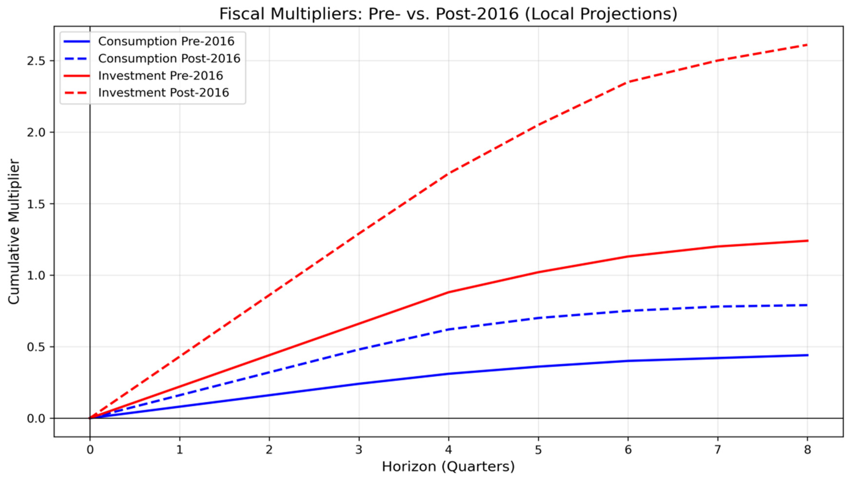
A key policy question is whether the ambitious economic reforms initiated under Vision 2030 have altered the effectiveness of fiscal spending. To address this, we split the sample at 2016Q1—the quarter in which Vision 2030 was formally announced—and re-estimated the multipliers for the pre- and post-2016 periods using the same local projection framework. Table 6 presents the results for the four- and eight-quarter horizons. In the pre-2016 era, the consumption multiplier at four quarters was a mere 0.31, rising only marginally to 0.44 after eight quarters. The investment multiplier was higher even then, at 0.88 and 1.24, respectively, but both figures are substantially smaller than their post-2016 counterparts. Following the launch of Vision 2030, the consumption multiplier more than doubles at the four-quarter horizon to 0.62 and reaches 0.79 at eight quarters. The post-2016 investment multiplier jumps to 1.71 at four quarters and an impressive 2.61 at eight quarters. These estimates suggest that the fiscal transmission mechanism has become more potent in the reform period, a finding consistent with Hypothesis H₃. Several factors could explain this enhancement. First, Vision 2030 has been accompanied by improvements in public financial management and project execution, which may have reduced implementation lags and cost overruns. Second, the diversification agenda has fostered a more dynamic non-oil private sector, potentially increasing the absorptive capacity for public investment. Third, the shift in spending composition toward high-impact infrastructure (such as NEOM, the Red Sea Project, and renewable energy ventures) may generate larger spillovers to the broader economy than traditional capital expenditure. Figure 3 visually contrasts the pre- and post-2016 multiplier paths, highlighting the stark difference in the post-reform period.

5.6. Time-Varying Evidence from Rolling Windows

To examine whether the increase in multipliers occurred abruptly or gradually, we computed rolling-window estimates using a fixed 20-quarter window rolled forward one quarter at a time. Figure 4 displays the evolution of the four-quarter cumulative multipliers for consumption and investment over the sample period. The vertical dashed line marks the launch of Vision 2030. Before 2016, both multipliers exhibit moderate fluctuations but remain within a relatively narrow band—consumption between 0.2 and 0.5, and investment between 0.6 and 1.2. Starting in 2016, however, the investment multiplier begins a steady upward climb, exceeding 2.0 by 2020 and remaining elevated through the end of the sample. The consumption multiplier also shows a modest increase after 2016, though it stays below 0.8 throughout. This rolling-window evidence reinforces the structural break analysis and indicates that the enhanced effectiveness of government investment is not a one-off phenomenon but rather a sustained change that coincides with the implementation of Vision 2030 reforms.

5.7. Variance Decomposition: How Much Do Fiscal Shocks Explain?

The final piece of the empirical puzzle concerns the relative importance of different structural shocks in driving fluctuations in non-oil GDP. Table 7 reports the forecast error variance decomposition at selected horizons from one to twelve quarters. In the very short run (one quarter), shocks to non-oil GDP itself account for the largest share (76.1%) of its own variance, reflecting the influence of idiosyncratic factors and measurement noise. Government investment shocks already explain a notable 12.7% of the variance, more than government consumption (3.8%) and oil-related shocks combined. As the forecast horizon lengthens, the contribution of investment shocks grows steadily, reaching 18.9% at four quarters, 24.3% at eight quarters, and 27.5% at twelve quarters. In contrast, the share attributable to consumption shocks rises only modestly to 8.9% after three years, while the own-shock contribution declines to 46.5%. This decomposition reveals that, over business cycle frequencies, government investment is a quantitatively important driver of non-oil economic activity in Saudi Arabia, whereas government consumption plays a secondary role. The variance explained by oil price and oil output shocks remains relatively small throughout, suggesting that, conditional on the fiscal variables included in the model, the direct impact of oil market developments on the non-oil sector is limited. This finding supports Hypothesis H₄: fiscal shocks are not crowded out by oil price fluctuations; instead, they exert an independent and substantial influence.

5.8. Summary of Key Findings and Their Implications

In summary, the empirical analysis yields four robust conclusions. First, government investment in infrastructure generates fiscal multipliers that are both larger and more persistent than those associated with government consumption. At an eight-quarter horizon, the investment multiplier is approximately three times the size of the consumption multiplier. Second, this pattern holds across alternative estimation techniques, including VECM-based impulse responses and local projections. Third, the effectiveness of fiscal spending has increased markedly since the launch of Vision 2030, with the post-2016 investment multiplier exceeding 2.5 at the eight-quarter mark. Fourth, government investment shocks account for a sizeable fraction of the forecast error variance of non-oil GDP, underscoring their macroeconomic significance. From a policy perspective, these results provide empirical justification for the strategic reallocation of public expenditure away from current consumption and toward capital formation. Under Vision 2030, the Saudi authorities have prioritised mega-projects and infrastructure development; our findings suggest that this shift is likely to yield higher non-oil growth per riyal spent, thereby accelerating the diversification of the economy away from hydrocarbons. Future research could extend this analysis by examining sectoral heterogeneity in multipliers or by employing narrative identification methods to further isolate exogenous fiscal shocks.

6. Conclusions

This study has provided a rigorous empirical assessment of the differential effects of government consumption and infrastructure investment on non-oil economic activity in Saudi Arabia, a context of profound structural transformation under Vision 2030. The relatively modest impact multiplier for investment (0.47) indicates that large-scale infrastructure projects take time to build momentum. A complementary, temporary allocation to current spending that supports project execution and local content may help bridge the short-run output gap, ensuring a smoother intertemporal fiscal path under Vision 2030. The evidence underscores the critical importance of expenditure composition in shaping fiscal policy outcomes within resource-dependent economies pursuing diversification. The findings carry immediate relevance for the design of growth-oriented fiscal frameworks in the Gulf region and beyond, particularly where public investment is tasked with catalysing private sector development and reducing hydrocarbon reliance. Beyond the specific numerical estimates, the analysis reaffirms a broader principle: the transmission of fiscal policy is not invariant to the nature of public outlays. Capital formation, especially when embedded in a credible long-term reform agenda, appears capable of generating sustained output responses that current spending alone cannot replicate. This insight challenges simplistic aggregative approaches to fiscal multiplier estimation and calls for greater granularity in both academic research and policy evaluation.

Nevertheless, the conclusions presented here are necessarily circumscribed by data availability and methodological choices. The use of quarterly national accounts, while an advance over annual series, still relies on proxies for fiscal shocks and imposes identifying assumptions that, though conventional, warrant ongoing scrutiny. Moreover, the sample period encompasses extraordinary global disruptions, including the COVID-19 pandemic, which may confound the attribution of post-2016 multiplier changes solely to domestic reforms. Future work could fruitfully extend this analysis by employing narrative identification of exogenous fiscal policy shifts, exploring sectoral heterogeneity in multiplier effects, or examining the interaction between public capital formation and private investment at the firm level. Cross-country comparative studies within the GCC would also illuminate whether the patterns observed for Saudi Arabia generalise to other oil-exporting economies undergoing similar transitions.

Under the maintained identification assumptions, the evidence suggests that prioritising infrastructure investment over current consumption is associated with larger and more persistent non-oil GDP growth, supporting the strategic direction of Vision 2030.

It should be noted that the large long-run investment multipliers estimated here are conditional on the sustained availability of fiscal resources. Saudi Arabia’s public debt-to-GDP ratio, though rising from its 2014 low to about 25% in 2023, remains among the lowest in the G20, and the IMF (2023) assesses the Kingdom’s fiscal space as ample, supported by substantial sovereign net worth and low borrowing costs. Under a fixed exchange rate and with credible medium-term fiscal frameworks, the net welfare gain from well-targeted public investment is likely to remain positive even when debt dynamics are considered. Nevertheless, the precise interaction between high multipliers and debt sustainability warrants further research, particularly as mega-project outlays accelerate.

The rolling-window evidence suggests that investment multipliers are larger during periods of low oil prices and economic slack, consistent with state-dependent effects found in the GCC literature. A formal threshold VECM analysis is beyond the sample size constraints of this study but represents an important direction for future work.

In sum, as Saudi Arabia continues to implement the far-reaching objectives of Vision 2030; the evidence presented here suggests that the strategic emphasis on infrastructure investment is well aligned with the goal of accelerating non-oil growth. Continued monitoring of fiscal effectiveness, coupled with refinements in public investment management, will be essential to fully realise the diversification dividends of this historic policy reorientation.