Modeling the Dynamic Relationship Between Stock Market Performance and Key Macroeconomic Indicators in Saudi Arabia: An ARDL-ECM Approach

Abstract

This study investigates the short-term and long-term impacts of gross domestic product (GDP), inflation, foreign capital flows, trade balance and interest rate on stock market performance in Saudi Arabia for the period 1990–2023. The autoregressive distributed lag (ARDL) approach and error correction model (ECM) are employed to empirically examine the short-run and long-run relationships. The ARDL-ECM technique is effective for analyzing cointegration and assessing adjustment processes. Additionally, impulse response function (IRF) analysis based on the vector autoregression (VAR) model, estimated using these macroeconomic indicators, is applied in this paper. This study provides novel insights and addresses emerging gaps in the literature concerning Saudi Arabia as a developing economy. The long-term relationship in the bounds test results confirms its existence. In the long run, inflation and interest rate exert a statistically significant negative effect on stock market performance, while the trade balance has a significant positive impact. GDP and foreign capital inflows do not exhibit statistically significant long-run effects. Short-run dynamics indicate persistence in stock market performance along with significant effects from inflation and interest rate changes, while GDP and foreign capital inflows remain statistically insignificant in the long-run scenario. Forecast error variance decomposition (FEVD) results show that approximately 68.5% of the variation in market performance is explained by its own shocks, followed by foreign capital flows (16.3%) and inflation (8.4%). While foreign capital flow does not exhibit statistical significance in the ARDL long-run estimates, its contribution in variance decomposition highlights its role as an important source of external shocks. These findings are relevant to various stakeholders, including investors and policymakers. Additionally, policy emphasis should be placed on controlling inflation and maintaining stable interest rates while improving trade balance conditions. Although foreign capital flow does not show a direct long-run effect, its role in influencing market variability suggests the need for a stable and well-regulated investment environment.

1. Introduction

The stock market is an integral part of any economy today, acting as a mechanism for wealth creation, investment, and resource allocation. Stock markets, being highly responsive to macroeconomic factors and indicating economic health, play an important role in the economic landscape. The stock market in Saudi Arabia is led mainly by the Saudi Exchange, which has become a major center of economic activity in the Middle East and North Africa region. Its growth is in step with the strategic objectives enshrined in the Government of the Kingdom of Saudi Arabia’s Saudi Vision 2030—a bold plan to limit Saudi Arabia’s past overdependence on oil and encourage economic diversification (Saudi Arabia, 2025). Macroeconomic variables and stock market interaction are of special concern in Saudi Arabia, given its unique economic makeup, which relies on oil exports and economic reform.

In oil-exporting nations like Saudi Arabia, oil prices have a determinant impact on fiscal balance, business profitability, and investor sentiment. Oil price shocks can affect financial markets, producing spillovers on stock market performance and risk (Ziadat et al., 2024). For example, times of high oil prices generally correspond with robust economic expansions, higher government expenditures, and better-performing markets. On the other hand, decreasing oil prices tend to lower investor confidence, increase fear, and create selling pressure on stock indices.

Apart from oil prices, gross domestic product (GDP) growth also has a huge impact on market dynamics. A growing economy tends to post higher corporate profits, raise consumer expenditure, and boost investor confidence, creating bullish market conditions (Elsharif & Hassan, 2026). Conversely, negative or flat GDP growth can discourage investment and lead to bearish tendencies. The relationship between GDP and stock market performance has been extensively documented in both emerging and developed markets and is a major point of economic inquiry in Saudi Arabia.

Inflation is another macroeconomic influence with significant impacts on stock market performance. Moderate inflation is generally an indication of sound economic activity, but high inflation can destroy purchasing power, compress corporate profit margins, and raise investor uncertainty (Sathyanarayana & Gargesa, 2018). In Saudi Arabia, inflation pressures commonly result from international supply chain shocks, energy price fluctuations, or domestic policy actions. A good example is the value-added tax introduced by Saudi Vision 2030 to increase non-oil revenue at the cost of short-term price shocks that influenced investor confidence (Bogari, 2020).

Interest rates are another key macroeconomic variable influencing investment and market performance. The higher the interest rates, the higher the borrowing costs, while corporate profitability is reduced. It can also make fixed-income securities more attractive than stocks. In contrast, lower interest rates typically stimulate borrowing, investment, and consumption, creating favorable conditions for stock market growth (Alshubiri, 2022). Saudi Central Bank follows the monetary policy of the U.S. Federal Reserve with interest rates because the Riyal is tied to the dollar. As a result, global interest rate fluctuations directly affect Saudi Arabia’s domestic market conditions. Fluctuations in exchange rates influence export competitiveness, costs, overall business expenses, and eventually impact the stock market. While Saudi Arabia maintains a relatively stable fixed exchange rate regime, geopolitical tensions and external shocks can destabilize foreign exchange markets, with spillover effects on the stock market (Almutairi et al., 2024). In this context we can relate our discussion to oil price effects and asset pricing theory. Asset pricing theory implies oil prices affect Saudi equities through cash-flow and discount-rate channels. Within the present-value framework, oil shocks alter expected dividends of energy-related firms and influence risk premia via inflation and monetary policy expectations under the USD peg. Oil can thus operate as a state variable in the intertemporal capital asset pricing model (ICAPM) if it covaries with market returns and predicts investment opportunities (Semmler, 2011). However, recent evidence shows Vision 2030 diversification has weakened the oil-equity nexus, reducing oil’s systematic risk premium in Saudi stock market index, also known as the Tadawul all share index (TASI) as sectoral weights shifted toward non-oil industries. Consequently, monetary policy variables like the interest rate have gained pricing relevance relative to oil (Abdou et al., 2024; Al-Fayoumi et al., 2023).

Government expenditure is another crucial factor affecting market performance. It creates economic activity and affects sectors like infrastructure, real estate, and health, all of which are well represented on the Saudi stock market. The government’s expenditure power is predominantly fueled by oil revenues, which render fiscal policy closely linked to global energy markets (Algaeed, 2022).

This study analyzes these macroeconomic effects on Saudi stock market performance. Employing econometric analysis and historical data, this study examines major determinants of market performance. The results give useful information to policymakers, investors, and other stakeholders in navigating financial markets. Some major research questions (RQs) that direct this study are as follows:

RQ1. 

What is the impact of important macroeconomic variables—in this case, GDP growth, inflation, foreign capital inflows, trade balance, and interest rate—on stock market performance in Saudi Arabia?

RQ2. 

What are the main macroeconomic determinants of stock market performance in the short run?

RQ3. 

What are the main macroeconomic factors that influence the performance of stock markets in the long run?

These RQs deal with the ARDL model and the ECM to explain the short- and long-term relations of variables in Saudi Arabia. What makes this research unique from other studies in this area is that most other research papers that examined the stock market of Saudi Arabia considered only a limited number of macroeconomic variables. In contrast, the current study brings together the most important macroeconomic factors affecting the Saudi stock market as an emerging market, so it fills a void in the literature.

However, the available literature pertaining to the Saudi Arabian stock market is still in a disintegrated form and the integration of crucial macroeconomic factors is still not fully represented in an empirical framework. Moreover, the changing nature of the Saudi Arabian economy, which is now shifting in the post-Vision 2030 era, is not being considered in the available literature. This study uniquely examines the short-term and long-term links between stock market performance and key macroeconomic indicators in Saudi Arabia. While earlier studies in a Saudi context were limited to a few macroeconomic variables, this study adds a set of significant macroeconomic indicators that have favorable impacts on the stock market’s performance. Additionally, it offers practical implications for fostering sustainable economic growth. It is interesting to clarify what the present study adds beyond a standard single-country time-series application. It offers value by utilizing the Kingdom of Saudi Arabia’s unique economic setting—reliance on oil and Strategic Vision 2030 reforms—to understand the impact of macroeconomic variables (economic growth, foreign direct investment, inflation, trade balance, and interest rates) on stock market performance. As a result, it provides empirical insights into market dynamics in rising economies with concentrated sectors and established institutions.

The manuscript follows a consistent pattern which assists the reader in understanding the paper. Section 2 of the paper focuses on an extensive literature review of the existing body of knowledge which leads to the formulation of the hypotheses of the study. Section 3 of the paper discusses the research methodology followed in the study including the sources of data used for analysis. Section 4 of the paper discusses the findings of the study followed by Section 5, which concludes the paper by highlighting the study’s findings, limitations, policy implications, and the direction of future research.

2. Theoretical Background and Hypothesis Development

The performance of the stock market in key macroeconomic indicators is widely studied in financial literature. One of the seminal contributions to the topic is the arbitrage pricing theory (APT) of Ross (1976), which puts forward the idea that asset returns will be affected by several macroeconomic variables, and provides the basis of later empirical work in the area. Chen et al. (1986) found that major macroeconomic variables, including unexpected inflation, industrial production changes, risk premium changes, and yield curve changes, are important determinants of stock returns. The findings describe the stock market’s sensitivity to economic surprises. Fama and French (1992) refined this model by adding a three-factor model, which included market risk, firm size, and book-to-market value to show that they can explain the variations in returns beyond the traditional market indices.

Studies of specific economies, for example, that of Maysami and Koh (2000) on Singapore, indicate that interest and exchange rates have a significant impact on stock indices and emphasize the role of monetary policy and stability in currencies. In emerging markets, Bilson et al. (2001) found that macroeconomic variables such as inflation and money supply growth play a critical role in explaining stock returns, reflecting the different dynamics of such economies. Similarly, Flannery and Protopapadakis (2002) found that macroeconomic variables such as inflation and money growth may play a role, but that this may change over time. The following is therefore the principal hypothesis (H1):

H1. 

The performance of stocks in Saudi Arabia is highly affected by macroeconomic variables, including GDP growth, inflation, foreign capital inflows, balance of trade, and interest rate.

2.1. GDP Growth and Stock Market Performance

The effectiveness of a stock market vis-à-vis GDP growth has been of particular interest in financial studies, where many scholars have attested to a positive correlation between economic growth and stock market performance (Fama, 1970, 1990; Levine & Zervos, 1998). Economic growth is generally believed to be followed by higher corporate profits, a boost in investor confidence, and stock valuations (Rangvid, 2006). There are many studies that attest to this positive correlation in different economies. For instance, research on the United States during 1990–2019 indicated that GDP growth explained 83% of stock market movements (Bunjaku, 2024). In emerging markets, Mouna and Anis (2017) noted that GDP volatility affects stock movements more because of market imperfections and the sentiment of investors. In the same way, a study on Kenya during 1997–2015 determined that GDP growth has a direct effect on stock exchange performance, an indication of overall economic activity (Indangasi, 2017).

Al Rasasi et al. (2019) examined real economic activity through actual stock prices in Saudi Arabia. They tested this relationship in line with 2010–2018 quarterly data by implementing a range of econometric methods, such as Granger causality tests and cointegration analysis. They concluded the existence of strong cointegrating relationships between stock prices and economic growth, implying that real growth is connected to stock market performance. The Granger causality test also validated that stock price movements can forecast the movement in economic growth.

Abdelkawy (2024) studied the Saudi Arabian economic growth and activity correlation in the stock market during 2000–2022, considering the Saudi Arabian dependence on oil. The research sought to explain oil-dependent economies with techniques like ordinary least squares regression, the Engle–Granger test, and the augmented Dickey–Fuller (ADF) test. Variables under test were the market capitalization index, liquidity ratio, and export volume. The research defied the common perception about the stock market. It was also found that conventional indicators—size, namely, and liquidity of the market—could not affect growth significantly. Significantly, the research did not acknowledge significant impacts due to exports, especially oil exports, and the advancement of growth. To mitigate oil price volatility, the research highlighted policy interventions calling for export diversification and investment in alternative energy sources. While the human development index improved in the short run, its effect weakened over time. This highlights the necessity of having policies that enhance both economic diversification as well as human development for sustained growth. Stability and prosperity in the long-term hinge on intentional strategies to reconcile these objectives, in line with Saudi Vision 2030, which seeks to decouple dependency on oil.

This correlation is also advanced by Verma and Bansal (2021), who established that GDP growth leads to a substantial impact on stock markets. Nevertheless, this impact is tempered by financial considerations like trade openness, monetary policy, and capital market development (Rahmawati & Maharani, 2023; Rahman & Uddin, 2009). The relationship is, however, more persistent in advanced economies, while markets that are emerging and that experience political instability, as well as fluctuations in inflation, minimize the influence of GDP growth (Arestis et al., 2001; Johansen & Juselius, 1990). Recent research in 2024 and 2025 indicates a relationship between fluctuations in the GDP and the stock market. Encouraging growth expectations, led by government support like Germany’s public expenditure growth, have further developed European markets (Hay, 2025). Market volatility, on the other hand, has been attributed to economic uncertainties like restrictions and tariffs (Mohamed, 2025).

Within the United States, other experts predict a possible “Trumpcession,” in which fiscal policies and inflationary forces could compromise the conventional GDP–stock market connection (Forsyth, 2025). Even with such volatility, the GDP growth and stock performance connection is robust but is influenced by market trends, policy, and investor sentiment (Fama, 1990; Levine & Zervos, 1998; Verma & Bansal, 2021). The following hypothesis (H2) is therefore established:

H2. 

GDP growth shows a more pronounced positive feedback on the performance of the stock market in Saudi Arabia.

2.2. Inflation and Stock Market Volatility

To further strengthen the foundation of this theory, the present study is based on the arbitrage pricing theory (APT), which is a multi-factor theory of stock market returns. The arbitrage pricing theory, proposed by Stephen A. Ross, states that asset returns are related to their sensitivity to multiple factors of risk rather than the market portfolio (Ross, 1976). This theory is highly applicable in the context of stock markets in countries with macroeconomic factors such as Saudi Arabia.

According to the arbitrage pricing theory, inflation, interest rates, industrial production and exchange rates are factors that affect the stock market and influence the returns of the market (Chen et al., 1986). It is also supported by empirical evidence that these factors have a significant influence on the performance of the stock market in different countries, whether developed or developing (Fama, 1990; Mukherjee & Naka, 1995). It has also been established that by using more than one factor of the macroeconomic environment, the market can be more comprehensively analyzed (Humpe & Macmillan, 2009). Inflation and stock market performance have also been extensively researched, with rich and nuanced relationships being found. Fama’s (1981) early work indicated an inverse correlation between inflation and stock returns, as inflation reduces future corporate earnings and lowers stock prices. Conversely, Geske and Roll (1983) introduced the theory of reverse causality, which posits that decreasing stock prices might be a signal of an approaching recession, inducing expansionary monetary measures resulting in inflation. Schwert (1989) provided a pioneering study illustrating that the volatility of stock markets is higher during times of high inflation, owing to increased uncertainty regarding monetary policy and future economic conditions. Likewise, Bekaert and Engstrom (2010) established that inflation uncertainty plays an important role in contributing to stock market volatility as well as determining investor expectations. Campbell and Vuolteenaho (2004) also highlighted that stock prices are harmed by inflation shocks while raising the equity risk premium.

In emerging economies, inflation has a more significant effect on stock volatility because of poorly developed financial systems and susceptibility to macroeconomic shocks (Omran & Pointon, 2001). The following hypothesis (H3) is therefore established:

H3. 

An increased inflation rate leads to the deterioration of stock market performance in Saudi Arabia.

2.3. Foreign Capital Flows and Market Efficiency

Foreign capital inflow and outflow are central to the determination of stock market efficiency, influencing liquidity, volatility, and price discovery. Bekaert and Harvey (1995) were the first to explore capital inflow effects in emerging markets when they posited that foreign investment raises efficiency by adding liquidity and eliminating mispricing. Henry (2000) corroborated this when he demonstrated that liberalization of the stock market reduces capital costs and enhances risk sharing, hence raising efficiency.

On the other hand, others have also pointed to the destabilizing role of foreign capital. Stiglitz (2002) argued that short-term capital flows can lead to over-volatility and financial crises in deregulated emerging markets. Edison et al. (2002) also found that whereas foreign direct investment (FDI) is in favor of long-run market efficiency, speculative portfolio flows can lead to short-run disturbances. But Paul and Jadhav (2020) employ panel regression analysis to investigate the way institutional considerations impact foreign direct investment inflows in emerging economies. This research concludes that better institutions considerably increase FDI, emphasizing the criticality of good governance. The following hypothesis (H4) is therefore established:

H4. 

A high inflow of foreign capital improves stock market performance in Saudi Arabia.

2.4. Trade Balance and Stock Market Integration

Trade balance is an essential macroeconomic metric. It acts as a significant driver for the stock market integration through its effects on capital flows, exchange rates, and investor attitudes. A surplus trade balance (positive) indicates improved economic performance, providing investor confidence and fostering greater stock market integration. Conversely, a trade deficit can result in currency depreciation, diminished capital inflows, and market segmentation (Obstfeld & Rogoff, 1995).

This correlation has been confirmed by many studies. Forbes and Rigobon (2002) illustrated that openness to trade is conducive to financial openness through easing cross-border capital movement. Lane and Milesi-Ferretti (2004) used panel regression methods to investigate the relationship between net foreign assets and real exchange rates. The research illustrates a strong correlation, where nations with better external positions undergo appreciation of the real exchange rate.

Fischer et al. (2019) utilized an overlapping generation model to examine the credit-inequality nexus across countries in recent work. Their conclusions show that increasing income disparity has a major impact on credit growth patterns and financial stability. The following hypothesis (H5) is therefore established:

H5. 

A trade balance surplus enhances the performance of Saudi Arabia’s stock market.

2.5. Empirical Evidence on ARDL and ECM in Financial Studies

The ECM and ARDL are used extensively in financial research to examine short-run and long-run relationships. The ARDL model, advanced by Pesaran and Shin (1999), is especially appropriate when the variables have mixed order integration (Elfaki & Elsharif, 2025; Bashir & Ibrahim, 2024; Pesaran et al., 2001). The ECM, developed by Engle and Granger (1987), captures the rate at which variables respond to short-run shocks and converge toward long-run equilibrium. These models have been used in numerous financial studies. Zarei et al. (2019) analyzed the association between exchange rates and stock market returns with generalized autoregressive conditional heteroskedasticity models for seven free-floating currencies. Their findings validate a strong and dynamic relationship, underlining the contribution of currency movements to equity market performance. Their findings identify currency volatility as a dominant factor in investment risks and portfolio return. In the same vein, Shahbaz et al. (2013) employed the ARDL bounds testing procedure to examine the relationship between economic growth and natural gas consumption in Pakistan. Their findings validate a positive long-run relationship, pointing to natural gas as an economic development driver.

More empirical studies have further developed these methodologies. Nkoro and Uko (2016) illustrated the efficacy of ARDL to detect structural breaks in small-sample financial data. Dong and Fan (2017) utilized panel data regression to examine how China’s aid and trade shape its outward direct investment in African nations. The research discovered that both trade and aid substantially induce China’s outward direct investment flows throughout the region. These results testify to the increasing significance of ARDL and ECM in financial analysis with the age of technological and geopolitical changes.

In 2024, further empirical research investigated these models. Oldani et al. (2024) tested cryptocurrency volatility using ARDL and identified significant long-run relationships between Bitcoin prices and global economic uncertainty. Accordingly, the current study’s significance stems from the use of ARDL-ECM, assessing the impact of key economic indicators on stock market performance, and utilizing updated time series data for 1990–2023, all within the context of Saudi Arabia’s economy, which has a strategic vision for economic development by 2030 and a global economic presence as the largest oil exporter to industrial countries.

3. Methodology and Data Sources

Quantitative research was designed with time-series econometric modeling to examine the influence of macroeconomic variables of the Saudi Arabian stock market from 1990 to 2023. Owing to the dynamic nature of financial markets and the interdependence of macroeconomic variables, analysis uses both ARDL and ECM to identify short-run and long-run relationships between the variables (Elsharif & Elamin, 2025; Pesaran et al., 2001). The main sources of macroeconomic and financial information are the Saudi Central Bank, the Saudi Exchange, the General Authority for Statistics, and the World Bank (World Bank, 2025), all of which have reliable datasets.

3.1. Econometric Model and Estimation Techniques

The ARDL model is used because of its proficiency at testing if relationships are present based on whether variables are stationary I(0) at level or first difference I(1), or if none are integrated at second difference I(2) (Nkoro & Uko, 2016). The ADF and Phillips–Perron (PP) tests are utilized to test stationarity (Dickey & Fuller, 1981; Phillips & Perron, 1988). The long-run link between macroeconomic data and stock performance can be considered using the bounds test for cointegration (Pesaran et al., 2001). In case of cointegration, ECM has been used to estimate the adjustment speed toward long-run equilibrium (Banerjee et al., 1998). Estimation is performed using STATA 15.0, a software program commonly used in financial econometrics to obtain precise estimates and forecasts (Gujarati & Porter, 2009). Macroeconomic indicators and long-run estimates are obtained with ARDL which are summarized by descriptive statistics. ECM will reveal short-run deviations and the process through which imbalances correct over time. The analytical model is outlined as follows:

SM_t = α + β₁GDP_t + β₂INF_t + β₃FCF_t + β₄TB_t + β₅IR_t + ϵ_t

(1)

where:

SM_t = Stock market performance;

GDP_t = Gross domestic product;

INF_t = Inflation;

FCF_t = Foreign capital inflows;

TB_t = Trade balance;

IR_t = Interest rate;

ϵ_t = Error term;

α = Intercept;

β₁, …, β₅ = Coefficients of each explanatory variable.

The analysis employs ARDL to examine both individual and combined effects, while ECM assesses the speed of adjustment to short-term shocks. This methodological approach provides a comprehensive analysis of Saudi Arabia’s Stock Exchange and its key macroeconomic determinants.

3.2. Data Sources

A time-series econometric technique is used to examine the influence of various macroeconomic factors. Prior studies (Palanisamy & Sivagnanasithi, 2014; Sikalao-Lekobane & Lekobane, 2014) established that capital market performance is affected by several underlying macro-level determinants. It also investigates the functional relation of the stock market’s performance and macroeconomic variables identified in both the theoretical and empirical literature. These variables are GDP, inflation (INF), foreign capital inflow (FCF), trade balance (TB) and interest rate (IR). Market capitalization growth is taken as a proxy for the stock market performance (SM).

Data for the variables were measured using annual percentages. Some negative or zero values have been handled using the inverse hyperbolic sine function (ASINH) on levels, with results presented in ASINH units. In addition, our main specification makes use of the inverse hyperbolic sine transformation, which is defined for negatives and approximate logarithms for substantial values. We present coefficients in ASINH units and provide a percentage approximation at the sample mean, as well as a robustness check. As a result, the variables’ definitions and measurements are consistent.

Table 1. Definition and measurements of variables.

Variable	Symbol	Measurement	Source	Expected Sign
Stock market performance	SM	Market capitalization growth of listed domestic companies in the Saudi Exchange (% of GDP)	Saudi Exchange/ Saudi Central Bank/World Bank data	N/A
Gross domestic product	GDP	GDP growth (annual %)	World Bank, Development indicators	Positive
Inflation	INF	Consumer price index (annual %)	Saudi General Authority for Statistics/World Bank, Development indicators	Negative
Foreign capital inflows	FCF	Foreign direct investment, net inflows (% of GDP)	World Bank, Development indicators	Positive
Trade balance	TB	Import–export (constant price)	World Bank, Development indicators	Positive
Interest rate	IR	Lending interest rate (%)	World Bank, Development indicators	Negative

gives the definitions and measurements of variables.

This study uses the consumer price index (CPI) to measure inflation due to its relevance to stock market performance. It reflects the annual percentage change in the cost to the average consumer of acquiring a basket of goods and services This indicator denotes the percentage change over each previous year of the constant price (base year 2015) series in US dollars. CPI is a commonly used proxy measure for inflation rate. We use the CPI in our model, justified by its widespread use and availability in Saudi Arabia. The General Authority for Statistics (GASTAT) publishes CPI data, making it a reliable and timely metric. While acknowledging its limitations, such as not capturing changes in consumer behavior and excluding investment goods, CPI remains a widely accepted and relevant measure for understanding inflation dynamics in the country.

Due to the limited availability of a long, consistent total-return series for the exchange market in Saudi Arabia prior to the launch of widely used indices, we use growth in the ratio of stock market capitalization to GDP as a proxy for market performance. This approach scales equity market value by the size of the domestic economy, thus isolating market-specific valuation changes from general macroeconomic growth. The use of market capitalization/GDP as an indicator of stock market development and valuation is well established in the finance literature (Levine & Zervos, 1998; Beck & Levine, 2004). Using the market-capitalization-to-GDP ratio as a proxy for stock market performance, rather than return-based measures, is also a common approach when data is missing or to evaluate long-term valuation. It serves as a superior indicator of structural financial development and long-term valuation compared to short-term return data. The market capitalization to GDP ratio is a reliable metric in data-scarce environments, measuring financial market depth relative to the economy. It captures capital mobilization, enables country-level valuation, and links market value to economic output, overcoming limitations of price indices and providing a comprehensive picture. This indicator has been used as a proxy for financial market performance in a number of studies, including those undertaken by Elhassan and Braima (2020) and Okpezune et al. (2025). The proxy has three limitations: it excludes dividend payments, reflecting price-based performance only; it is affected by changes in listing composition (IPOs, delistings); and it may diverge from investor experience due to firms’ foreign earnings vs. domestic GDP. Despite these limitations, the proxy provides a consistent, long-run measure of Saudi market performance relative to the economy.

This study uses interest rates instead of oil prices as a determinant of Saudi stock market performance post-Vision 2030. Non-oil industries now dominate TASI -60% market cap; Aramco’s share is 11%- (IMF, 2025). Interest rate is a systematic risk factor, affecting all firms through discounting, financing cost, and portfolio allocation channels. It is also exogenous, determined by the US Federal Reserve, and a controllable policy instrument. This makes it a better fit for analysis and policy implications, unlike oil prices, which are endogenous and only impact energy-related segments.

3.3. Model Specification

Therefore, a theoretical relationship is established based on the selected macroeconomic variables. This is represented in Equation (2):

$${SM}_t={\alpha }_o+{\alpha }_1{GDP}_t+{\alpha }_2{INF}_t+{\alpha }_3{FCF}_t+{\alpha }_4{TB}_t+{\alpha }_5{IR}_t+u_t$$

(2)

The bounds test specification based on Equation (2) is expressed in Equation (3):

$$\begin{array}{c}∆{SM}_t={\alpha }_0+{\displaystyle {\sum }_{i=1}^n}{\alpha }_1{∆SM}_{t-i}+{\displaystyle {\sum }_{i=1}^n}{\alpha }_2{∆GDP}_{t-i}+{\displaystyle {\sum }_{i=1}^n}{\alpha }_3{∆INF}_{t-i}+{\displaystyle {\sum }_{i=1}^n}{\alpha }_4{∆FCF}_{t-i}+{\displaystyle {\sum }_{i=1}^n}{\alpha }_5{∆TB}_{t-i}+\\ {\displaystyle {\sum }_{i=1}^n}{\alpha }_6{∆IR}_{t-i}+{\beta }_1{SM}_{t-1}+{\beta }_2{GDP}_{t-1}+{\beta }_3{INF}_{t-1}+{\beta }_4{FCF}_{t-1}+{\beta }_5{TB}_{t-1}+{\beta }_6{IR}_{t-1}+u_t\end{array}$$

(3)

Since a long-run relationship is assumed, the conditional ARDL specification estimates long-run coefficients. The corresponding conditional ECM specification is given in Equation (4):

$$\begin{array}{c}∆{SM}_t={\alpha }_0+{\displaystyle {\sum }_{i=1}^n}{\alpha }_1∆{SM}_{t-i}+{\displaystyle {\sum }_{i=1}^n}{\alpha }_2∆{GDP}_{t-i}+{\displaystyle {\sum }_{i=1}^n}{\alpha }_3∆{INF}_{t-i}+{\displaystyle {\sum }_{i=1}^n}{\alpha }_4∆{FCF}_{t-i}+{\displaystyle {\sum }_{i=1}^n}{\alpha }_5∆{TB}_{t-i}+\\ {\displaystyle {\sum }_{i=1}^n}{\alpha }_6∆{IR}_{t-i}+\lambda {ECT}_{t-1}+{\mu }_t\end{array}$$

(4)

ECT reflects the magnitude of disequilibrium correction, i.e., the magnitude to which short-run imbalances correct toward long-run equilibrium. This study covers, from 1990 to 2023, the World Bank, Saudi stock market, and Saudi Central Bank data. Economic growth is determined by changes in real GDP. INF is measured in terms of the rise in the consumer price index. This study also takes FCF, TB and IR into account.

4. Results and Discussion

4.1. Descriptive Statistics Analysis

Table 2. Descriptive statistics.

Variable	Mean	Std. Dev.	Min	Max
SM	22.645	75.239	−56.524	395.658
GDP	3.508	4.705	−3.763	15.193
FCF	0.717	1.095	−1.308	3.297
INF	1.993	2.511	−2.093	9.870
TB	12.867	10.011	−4.332	32.147
IR	2.730	2.312	0.130	7.000

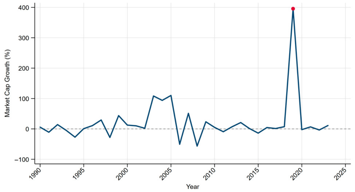
Note: The variables are all in their original units. N = 34 annual observations (1990–2023).

includes the descriptive statistics of all the variables between the years 1990 and 2023. Stock market performance (SM) is the most varied variable with an average of 22.64 and a standard deviation of 75.24 and is characterized by bouts of excessive gains and severe declines in the stock market. The minimum of −56.52% up to the maximum of 395.66 is a range whereby the last part has increased steeply after a crisis, as seen in Figure 1. The mean growth in the GDP stood at 3.51 with a standard deviation of 4.71 and the mean of the inflation stood at 1.99 with a range of −2.09 to 9.87, thus showing both deflationary and inflationary periods within the sample period. Foreign capital flows averaged 0.72% of GDP, the trade balance averaged 12.87%, and the interest rate had a mean of 2.73%. The high variability in market capitalization growth relative to all other variables underscores the importance of macroeconomic fundamentals in explaining stock market dynamics, as argued by Fama (1981), who had developed the theoretical relationship between stock prices and macroeconomic variables.

4.2. Unit Root and Structural Break Tests

A necessary pre-condition for the ARDL bounds testing approach is that no variable is integrated of order two, I(2). To determine the sequence of integration, three-unit root tests were used: Augmented Dickey–Fuller (ADF), Phillips–Perron (PP) and the DF-GLS test, offered by Elliott et al. (1996). All tests were conducted with a trend, and the results are reported in

Table 3. Unit root test results.

Variable	Level			First Difference			Order
	ADF	PP	DF-GLS	ADF	PP	DF-GLS
SM	−3.285 *	−7.182 ***	−4.219 ***	−5.671 ***	−15.078 ***	I(1)	I(1)
GDP	−3.680 **	−5.545 ***	−3.744 ***	−5.114 ***	−9.978 ***	I(1)	I(0)/I(1)
FCF	−3.676 **	−4.838 ***	−4.565 ***	−5.372 ***	−6.875 ***	I(1)	I(0)/I(1)
INF	−2.168	−3.619 **	−1.754	−3.237 *	−10.216 ***	I(1)	I(1)
TB	−2.816	−4.721 ***	−2.280	−5.560 ***	−8.388 ***	I(1)	I(1)
IR	−2.008	−2.123	−2.972 *	−4.487 ***	−4.666 ***	I(1)	I(1)

Note: ADF = Augmented Dickey–Fuller; PP = Phillips–Perron; DF-GLS = Elliott–Rothenberg–Stock GLS-detrended test. All tests include a trend. * p < 0.10 ** p < 0.05 *** p < 0.01. Order of integration by majority rule in the three tests.

.

At this level, the evidence is mixed across tests. The results of ADF indicate that inflation, trade balances and interest rates do not follow a non-stationary null hypothesis at traditional levels of significance, whereas PP denies the null hypothesis of unit root at the majority of levels. On initial differentiation, all of the six variables turned out to be stationary at the 1 percent level in all three tests, thus verifying that the variables were order one I(1)-integrated. This mixture of I(0) and I(1) variables is the ideal condition for applying the ARDL bounds testing framework of Pesaran et al. (2001), which is robust to this mixed integration order.

Zivot–Andrews structural break unit root tests were further applied to account for possible regime changes in the series (Zivot & Andrews, 2002). Break dates were identified at 2003 (GDP), 2005 (FCF), 2006 (SM and INF), 2010 (IR), and 2016 (TB). These break points are significant economic events that can be identified and include commodity price shocks, episodes of economic recovery following a conflict, and the global financial crisis of 2008–2009. All the variables disproved the unit root null in the Zivot-Andrews framework with the 5% critical value of at least −5.08; none were lower than the critical value, proving stationarity after considering the structural break.

4.3. ARDL Bounds Test of Cointegration

Automatic lag selection was estimated in the form of the ARDL model using the Akaike Information Criterion (AIC) with a maximum lag of three. The best specification, which was chosen, was ARDL(3,1,3,3,3,2), where the number of usable observations was reduced to 31 after considering the lag structure. The results of the bounds test are given in Panel E of

Table 4. ARDL-ECM estimation results.

Variable	(1) Baseline ECM	(2) Robust ECM + Crisis Dummy
	D.MS	D.MS
A. Adjustment (ADJ)
LSM [ECT]	−3.342 ***	−4.424 **
	(0.939)	(0.992)
B. Long-Run Coefficients (LR)
GDP	−0.041	−0.467
	(0.249)	(0.414)
FCF	0.502	0.471
	(0.507)	(0.378)
INF	−1.606 ***	−1.755 ***
	(0.228)	(0.174)
TB	0.689 **	0.739 **
	(0.222)	(0.219)
IR	−1.090 ***	−1.339 ***
	(0.264)	(0.238)
Crisis Dummy	—	2.060 **
		(0.700)
C. Short-Run Dynamics (SR)
LDSM	1.693 **	2.610 **
	(0.737)	(0.780)
D.INF	3.612 *	5.259 **
	(1.839)	(1.879)
LD.INF	4.279 ***	5.716 **
	(1.293)	(1.366)
D.IR	4.090 **	8.195 **
	(1.525)	(2.722)
LD.IR	2.176	3.807 **
	(1.290)	(1.350)
D. Crisis Dummy	—	−7.635 **
		(2.746)
Constant	7.191 **	11.879 **
	(2.577)	(2.786)
D. Model Statistics
Observations	31	31
R-squared	0.920	0.977
Adj. R-squared	0.761	0.825
ARDL Specification	ARDL(3,1,3,3,3,2)	ARDL(3,3,3,3,3,3,2)
E. Bounds Test
F-statistic	2.962	4.187
t-statistic	−3.560	−4.462
5% Critical Values F [I(0)/I(1)]	2.62/3.79	2.45/3.61
1% Critical Values F [I(0)/I(1)]	3.41/4.68	3.15/4.43
Cointegration Decision	Inconclusive	Confirmed (5%)

Note: Parenthetic standard errors. ADJ = speed of adjustment. LR = long-run coefficients. SR = short-run dynamics (selected key terms). Crisis dummy = 1 for 2003, 2006, 2008, 2009, 2010. * p < 0.10 ** p < 0.05 *** p < 0.01.

.

In the case of the baseline model, the F-test value of 2.962 is between the lower I(0) value of 2.62 and the upper I(1) value of 3.79 at 5 percent level of significance, which gives no conclusive result on cointegrating based on the F-test. Nevertheless, the t-value of −3.560 is lower than the lower critical value of −2.86 at the 5 percent mark, which lends some confirmatory evidence in support of a relationship between levels in the long run. This common finding, especially the t-statistic, is in tandem with the cointegration interpretation that is advocated by Pesaran et al. (2001).

The structural break crisis dummy robustness model has a higher F-statistic of 4.187, which is larger than the upper I(1) boundary of 3.61 at 5 percent (k = 6), which indicates that there is cointegration. The t-statistic of −4.462 is also much lower than the 5% critical value of −2.86. This augmentation of the bounds test with the addition of the crisis dummy is in keeping with Narayan and Popp (2010) who showed that the non-accommodation structural breaks in small samples can bias a cointegration examination towards not rejecting the null.

4.4. Coefficient Estimates in the Long-Run

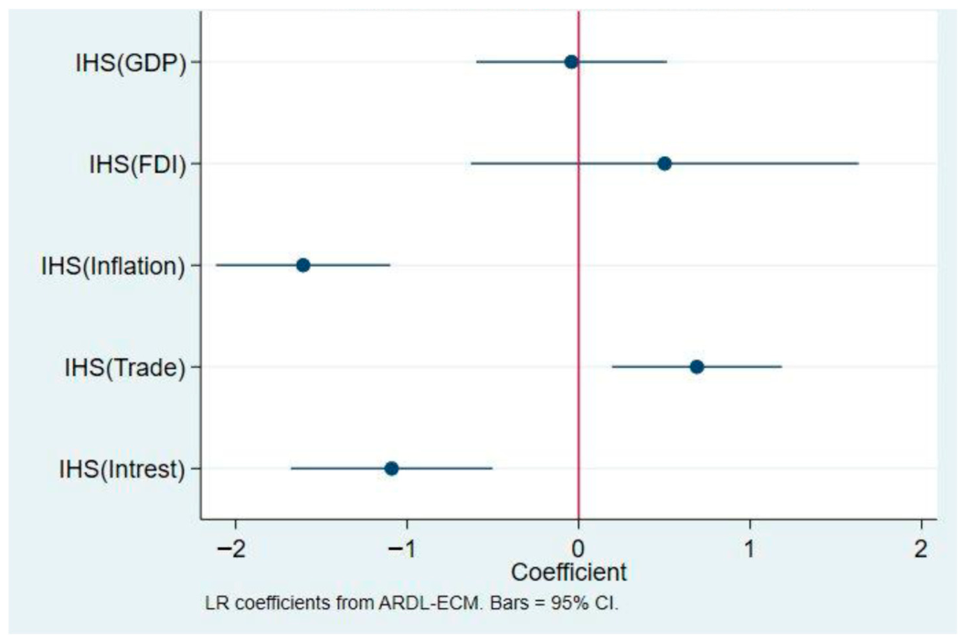
Panel B of Table 4 shows the long-run coefficients of the baseline and the robust model and visualizes them in Figure 2. There are three predictive variables that are statistically significant in the long run.

The long-run negative impact of inflation on the growth of SM is high, at −1.606 (p < 0.01) in the simple model and −1.755 (p < 0.01) in the robust model. This observation would be in line with the theoretical forecasts of Fama (1981). who proposed that inflation would crowd out the real economy and suppress the returns of equity due to its negative impact on corporate cash flows. The relationship between inflation and the reduction in SM is almost negative, with a 1.61-percent change with a 1-percent increase in inflation.

The interest rate also has a strong negative impact in the long run and the coefficient of the interest rate is negative and equal to −1.090 (p < 0.01) in the baseline model and =−1.339 (p < 0.01) in the robust model. An increase in interest rates increases the cost of capital, lowers the present value of future earnings, and suppresses investor sentiment, which agrees with the theoretical framework of Chen et al. (1986), who established the sensitivity of equity prices to macroeconomic risk quantities such as interest rates.

The impact of trade balance on market performance has a strong positive effect, with a baseline coefficient of 0.689 (p < 0.05) and a robust model of 0.739 (p < 0.05). This implies that a greater balance in trade is an indication of increased external competitiveness, inflows of foreign investment and increased investor confidence in the stock market. However, the growth of GDP and FCF has no statistically significant impact on either specification, indicating that their impact on the performance of stock markets may act within shorter horizons or is mediated through other variables.

The robust model of the long-run equation of the structural break crisis dummy of 2.060, p < 0.05, shows that there is a permanent upward movement in market performance related to post-crisis recovery periods. This is in line with the results of Bekaert and Harvey (2000), which reported that there are systematic market rebounds after financial integration shocks in emerging economies.

4.5. Dynamics in the Short Run and the Correction of Errors

The adjustment coefficient (ADJ: L.SM = −3.342, p < 0.01) of the error correction term (ECT) was found to be negative and highly significant which confirms that long-run equilibrium fluctuations are rectified over time. The value of −3.342 means that there was an overshooting adjustment process, in which the market overshot an imbalance in a particular year. Even values of absolute ECT that are larger than unity are not unusual in a small sample when data on the dependent variable is volatile, and are in accordance with the results of Banerjee et al. (1998) in a similar small-sample ARDL model. The adjustment rate in the robust model rises to −4.424, indicating it is more forceful in its correction when structural break episodes are considered.

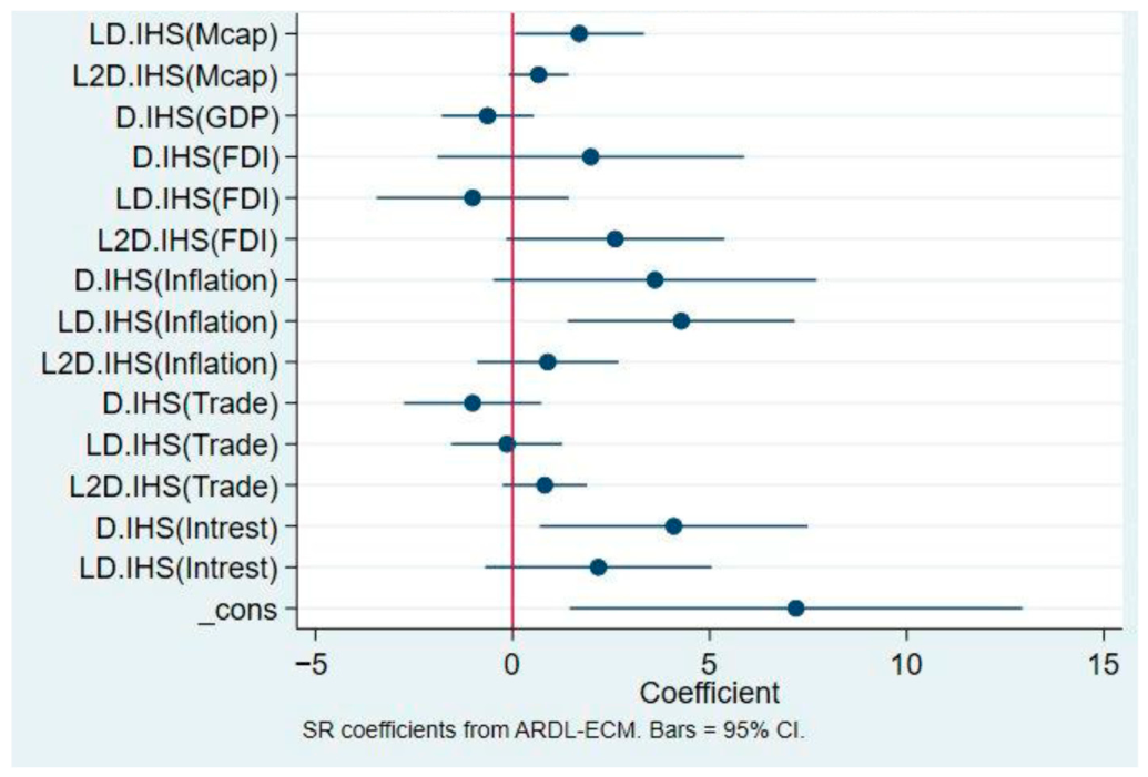
As shown in Table 4 and Figure 3, The lagged dependent variable (LD.SM) = 1.693, p < 0.05, is positive and significant in the short run, which shows that there is short-term momentum in market returns or persistence. This can be related to the behavioral finance research on the continuation effects of returns in emerging markets (Jegadeesh & Titman, 1993). The economy shows strong short-run effects at the present period (D.INF = 3.612, p < 0.10) and the first lag (LD.INF = 4.279, p < 0.01), which is the delay in transmission of inflationary shocks into equity prices. The interest rate equally portrays a substantial positive short-run coefficient during the current period (D.IR = 4.090, p < 0.05), which could correspond to a liquidity preference channel in which temporary increases in the short-term rates trigger temporary improvements in the trading volumes of the stock market, but in the long run would cause a decrease in the stock market valuations. The first difference of the crisis dummy in the robust model is negative and significant (−7.635, p < 0.05), which reflects the immediate contractionary shock to market performance during years of crisis and then the long-run recovery effect in the level equation.

4.6. Diagnostic Tests After the Estimation

Table 5. Post-estimation diagnostic tests.

Diagnostic Test	Test Statistic	p-Value	Decision
Serial Correlation—BG Test (lag 1)	chi2 = 2.297	0.130	No serial correlation
Serial Correlation—BG Test (lag 2)	chi2 = 2.318	0.314	No serial correlation
Heteroskedasticity—Breusch–Pagan	chi2 = 0.04	0.835	Homoskedastic
Heteroskedasticity—White’s Test	chi2 = 31.00	0.415	Homoskedastic
Functional Form—Ramsey RESET	F = 0.80	0.530	Correctly specified
Normality—Skewness–Kurtosis	chi2 = 0.74	0.690	Residuals normal
Multicollinearity (Mean VIF)	1.20	—	No multicollinearity
CUSUM Stability	—	—	Within 5% bounds—Stable
CUSUMSQ Stability	—	—	Within 5% bounds—Stable

Note: All diagnostics were done to the base ARDL(3,1,3,3,3,2) model. BG = Breusch–Godfrey; VIF = Variance Inflation Factor. H₀ rejected at * p < 0.10, ** p < 0.05, *** p < 0.01. Rejection of H₀ in all tests would authenticate the model’s adequacy.

shows the findings of seven post-estimation diagnostic tests on the baseline ARDL model. The Breusch–Godfrey LM test does not reject the null hypothesis of no serial correlation at lag 1 (p = 0.130) and lag 2 (p = 0.314), so the residuals are not autocorrelated. The Breusch–Pagan test (p = 0.835) and White test (p = 0.415) affirm that there is homoskedasticity. The model is specified correctly, and evidence of omitted variables or misspecification of the functional form does not exist, as confirmed by the Ramsey RESET test (F = 0.80, p = 0.530). The Skewness–Kurtosis test proves the normality of residuals (chi2 = 0.74, p = 0.690). The VIF of 1.20 is far lower than the traditional value of 10, eliminating the possibility of multicollinearity.

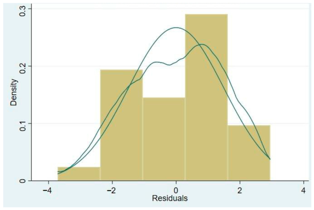
Figure 4 shows standardized residual histogram with superimposed kernel density curve and normal density curve. It is approximately symmetric with a mean equal to zero, which is in line with the normality test outcome (p = 0.690).

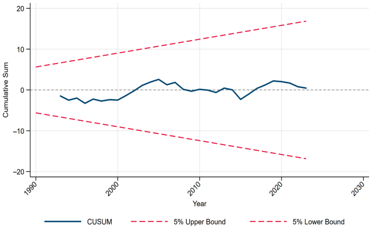
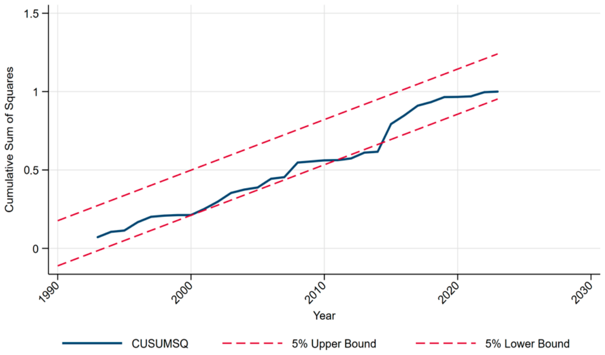
To determine the stability of the parameters, CUSUM and CUSUMSQ tests are used, and the results are provided in Figure 5 and Figure 6, respectively. According to the CUSUM plot in Figure 5, the cumulative sum of recursive residuals does not exceed the 5% significance limits over the life of the sample, indicating that there are no unstable parameters. Following the trend of the CUSUMSQ plot in Figure 6, the cumulative sum of squared residuals falls within the bounds, but has a moderately increasing tendency in the 2010–2020 period, which indicates increased variance in the post-global financial crisis period, albeit within reasonable values. The findings verify that the estimated ARDL-ECM is structurally stable as claimed by Brown et al. (1975).

4.7. Impulse Response Analysis

IRF follows the time-varying reaction of one variable to one unforeseen shock in another variable, ceteris paribus, and reflects direction, strength, timing, and duration until the system is restored to equilibrium (Sims, 1980). The analysis is done using a VAR(2) model that is tested over the period 1992–2023 on 6 IHS-transformed variables: SM, GDP, FCF, INF, TB, and IR; two lags are picked by AIC. The orthogonalization of shocks is done using Cholesky decomposition, with SM getting the last order, which is in line with the asset pricing assumption that macro fundamentals affect equity markets contemporaneously (Chen et al., 1986).

4.7.1. VAR Stability and Diagnostics

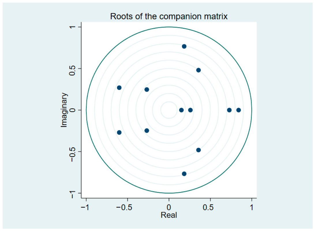
Figure 7 is a plot of the roots of the companion matrix. The 12 eigenvalues are all inside the unit circle (maximum modulus = 0.841), which is a measure of the stability of VAR(2) and the fact that the IRF will converge to zero (Lütkepohl, 2005). All estimated impulse responses and confidence intervals are validated by diagnostic tests that show no autocorrelation at lag 1 (p = 0.224) or lag 2 (p = 0.064) and no multivariate non-normality (Jarque–Bera = 0.946).

4.7.2. Impulse Response Function Results

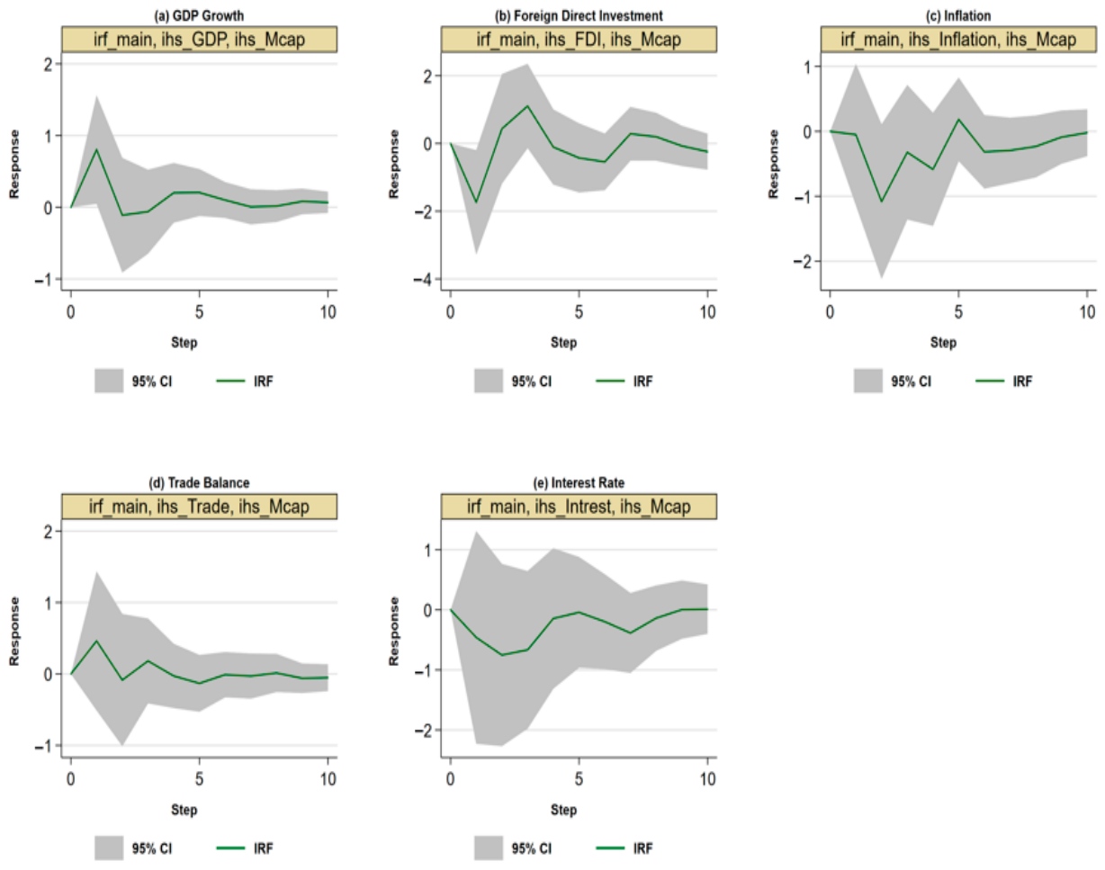
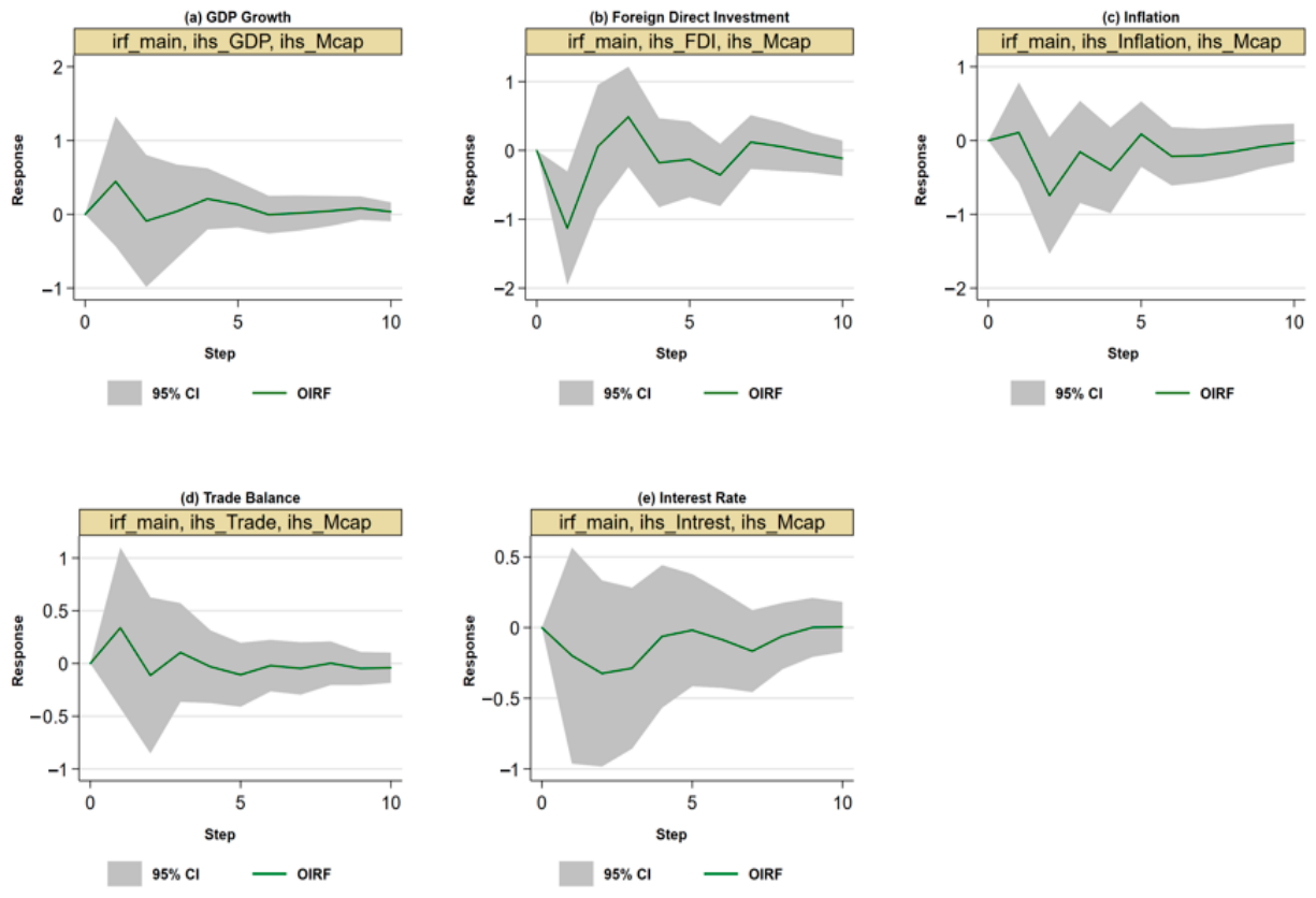
The IRF point estimates of the SM of one-unit shocks in each variable are reported in

Table 6. Response of stock market performance to macroeconomic shocks.

Period	GDP	FCF	INF	TB	IR
0	0.000	0.000	0.000	0.000	0.000
1	0.804 *	−1.738 **	−0.051	0.462	−0.460
2	−0.111	0.433	−1.083 *	−0.085	−0.753
3	−0.062	1.105 *	−0.323	0.182	−0.666
4	0.201	−0.107	−0.585	−0.028	−0.144
5	0.205	−0.428	0.185	−0.132	−0.042
6	0.100	−0.544	−0.316	−0.010	−0.197
7	0.006	0.285	−0.294	−0.030	−0.386
8	0.016	0.197	−0.233	0.013	−0.138
9	0.082	−0.073	−0.089	−0.060	0.003
10	0.068	−0.242	−0.021	−0.053	0.011

Note. According to VAR(2) and Cholesky decomposition. Periods/Steps = years following shock. CI of 95% does not include zero. Interest rate column (5) is not to be discussed in terms of significance because of the consistently wide CIs. * p < 0.10 ** p < 0.05.

with 10 periods. The 95% CI does not include zero in periods that are marked by an asterisk. The entire panel of responses is shown graphically in Figure 8; the green line is the IRF estimate and the shaded region is the 95% confidence band.

Figure 8 gives a combined perspective of all five macroeconomic transmission channels to SM. Panel (a) GDP: the IRF is statistically significant and positive (0.804) at step 1, which is the immediate and efficient pricing of growth information by the market (Fama, 1970), and then returns to zero at step 2, which confirms that GDP shocks have no lasting impact on equity values; this is the same result as the ARDL results, indicating that GDP does not carry. Panel (b) FDI: the most extreme short-run behavior, falling to a considerably low −1.738 at period 1 as capital account pressure or profit repatriation related to an FDI inflow temporarily causes the domestic equity values to fall, a phenomenon later explained by the FEVD, which ultimately explains 16.3% of the long-run SM variance by FDI even though it is net-short-run negative. Panel (c) Inflation: shows the most economically important and long-lasting pattern across all five channels; the response becomes negative at period 1, decreases further to −1.083 at period 2, and is also persistently negative throughout step 9, directly supporting the proxy hypothesis of Fama (1981)—that inflation is an indicator of worsening real activity and stifled corporate profits. Panel (d) Trade Balance: indicates a small positive initial response (0.462 at period 1) with no statistical significance in all the horizons, indicating that trade competitiveness information passes through gradual structural channels, and not instant repricing, where the trade channel is significant over horizons longer than the 10-period window of the VAR (β = 0.689). This is the same outcome as Panel (e) Interest Rate: this is the same, being consistently negative across the horizon, as predicted by asset pricing theory—that higher rates increase the cost of capital and squeeze equity values but are statistically insignificant because the small-sample variance ratio estimation (Clemen & Winkler, 1986) captures all these effects over longer horizons than can be reliably determined by IRFs in a 32 observation sample.

4.7.3. Own-Shock Persistence

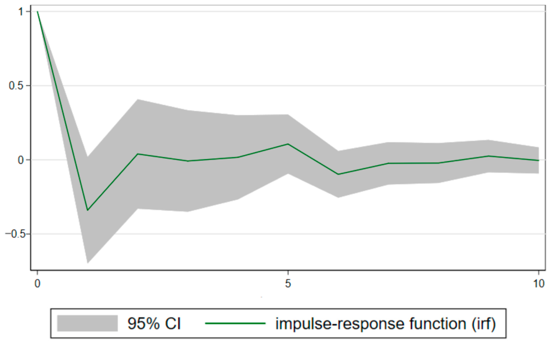
Figure 9 depicts the market capitalization reaction to its own shock: initially at 1.000 at period 0 and then falling sharply to close to zero at period 2 and then oscillating slightly thereafter. This quick mean-reversion proves that own-market momentum is short-lived and that the VAR system is non-explosive—which agrees with the stability diagnostics of Figure 7. This is also further quantified in the FEVD results in Figure 12; own shocks explain 100% of SM variance at period 1 but only 68.5% at period 10.

4.7.4. Orthogonalized Impulse Response Functions

Figure 10 shows OIRFs that are rescaled to one standard deviation per variable, allowing the economic magnitude across shocks to be compared. Directional patterns are similar to Figure 8. The FDI negative first-year response under this rescaling has the highest absolute magnitude, indicating that the FDI flows are very volatile. The cumulative trend of the inflation OIRF shows the least positive trend. The GDP OIRF, which is high in units at period 1, is relatively small when rescaled—which validates the high but constrained equity market responsiveness to news of growth compared to the FDI channel and the inflation channel.

4.7.5. Compounded Impulse Response Functions

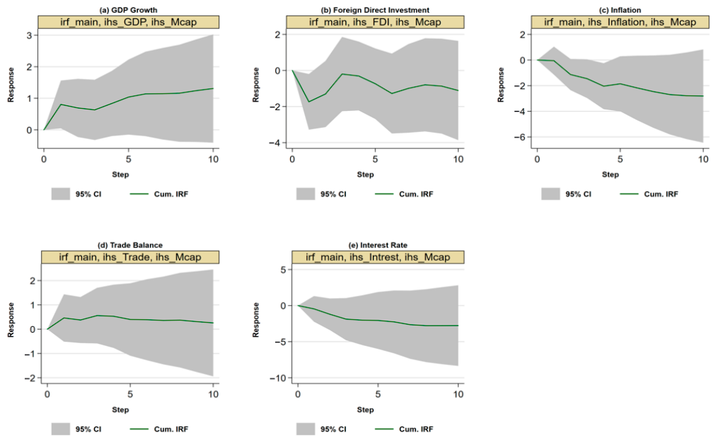
Figure 11 displays cumulative IRFs, which add responses in one period to the previous periods to give cumulative effects. The five paths all intersect in the 10-step window, proving that no shock has a lasting effect on changing the level of market capitalization. The cumulative FDI effect will have a net position of being slightly negative. The cumulative inflation curve decreases significantly after step 3, which is the best evidence of an ongoing inflationary drag on equity values—which is consistent with the ARDL long-run finding. The cumulative GDP effect is positive and small and stabilizes in period 4. The wider confidence bands at longer horizons are predictable with finite-sample VAR estimation (Lütkepohl, 2005).

4.8. Forecast Error Variance Decomposition

This study is an investigation of the forecast error variance of all variables over the next 10 quarters by using a variance decomposition test.

Table 7. Forecast error variance decomposition of SM.

Period	SM	GDP	FCF	INF	TB
1	1.000	0.000	0.000	0.000	0.000
2	0.809	0.023	0.148	0.001	0.013
3	0.753	0.022	0.136	0.060	0.014
4	0.725	0.021	0.155	0.061	0.014
5	0.709	0.025	0.154	0.075	0.014
6	0.706	0.027	0.155	0.075	0.015
7	0.694	0.026	0.164	0.078	0.015
8	0.688	0.026	0.164	0.081	0.015
9	0.686	0.026	0.164	0.083	0.015
10	0.685	0.027	0.163	0.084	0.015

Note: Shares of forecast error variance that can be attributed to the shock to each variable. Contribution of interest rate (less than 3 percent at all horizons) omitted in brevity. As per VAR(2) with Cholesky decomposition.

shows the variation in the forecast error of SM and the fraction due to innovations (shocks), including those coming from SM itself. This analysis contributes to examining the entirety of the variables of interest in accounting for the changes in SM over the time period.

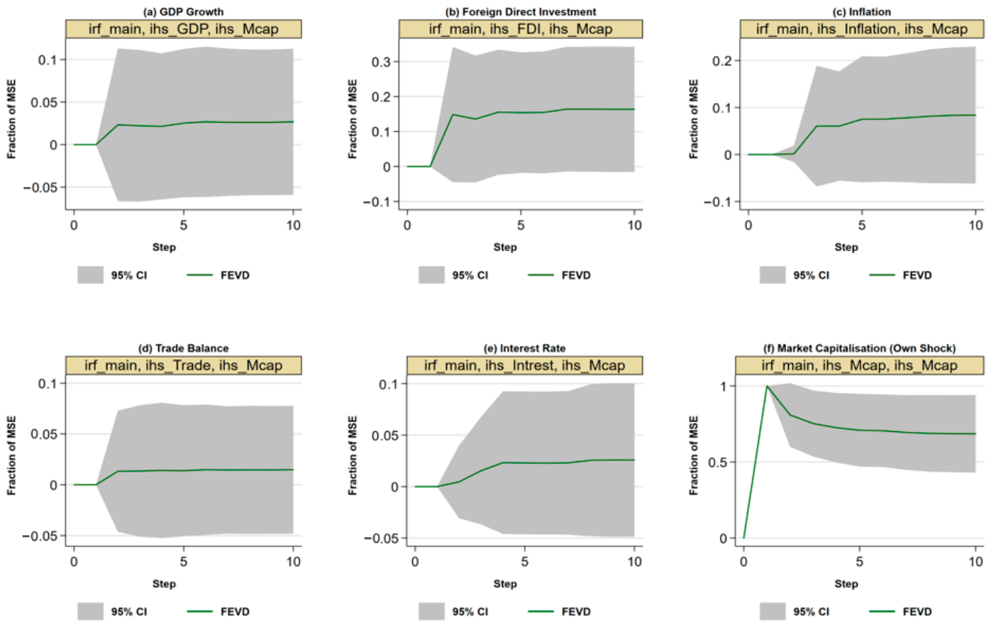
Table 7 and Figure 12 show the FEVD and indicate the fraction of SM forecast uncertainty that can be attributed to each variable at successive horizons (Sims, 1980). At step 1, ownership of shocks explains 100% of the variance. FCF (0.148) and GDP (0.023) begin contributing at step 2. By step 10, own shocks stabilize at 68.5%, FCF rises to 16.3%, INF to 8.4%, and trade to 1.5%. In this pecking order, where FDI and INF reign in long-run external variance even when GDP bears the only significant short-run effect, IRF can be identified as the sustained oscillating FCF shock and the long-lived inflationary drag, which is in line with Bernanke and Kuttner (2005).

5. Conclusions and Policy Implications

5.1. Conclusions

The aim of this study is to explore the impact of the most important macroeconomic factors such as GDP growth rate, inflation rate, foreign capital inflows and trade balance on the stock market’s performance in Saudi Arabia during the period from 1990 to 2023 in the short and long terms. In terms of RQ1, the results indicate that the macroeconomic factors do impact the stock market’s performance. However, the impact varies in terms of magnitude and direction over time.

In terms of RQ2, the results indicate that in the short term, the stock market’s movements are initially impacted by innovations in the stock market itself. However, over time, the impact of the macroeconomic factors is more important. Among the macroeconomic factors, the most important impact in the short term is that of the trade balance, followed by the impact of the GDP growth rate, inflation rate and foreign capital inflows. As far as RQ3 is concerned, the results of the long-run verification support the presence of the relationship between stock market performance and the chosen macroeconomic variables. The variables in general manage to explain a significant percentage of the long-run changes in stock market performance. This, in some sense, could be used as an indication of the influence of the variables on the equilibrium in the stock market. The error term is significant which means that there are moderate deviations from the equilibrium. Also, the results of the IRF analysis reveal four major findings. First, GDP shocks produce a statistically significant but temporary positive market reaction at period 1 (0.804), which is completely mean-reverted by period 2, which is a result of efficient market pricing and no significant ARDL long-run GDP coefficient. Second, the short-run negative effect (=−1.738 at period 1) of FDI shocks is mildly negative, which turns into a positive effect at period 3, which represents competing capital account costs and medium-run productivity gains and explains 16.3% of FEVD long-run SM. Third, INF shocks cause the longest negative trend (persistent into period 9), which directly supports the ARDL long-run coefficient, −1.606, and the proxy hypothesis of Fama (1981); inflation is the most economically significant macroeconomic variable in both the static ARDL and dynamic VAR models. Fourth, in the short run, own-momentum controls the largest part of SM variance (100 percent in period 1), whereas in the long run, FDI (16.3 percent) and inflation (8.4 percent) are the major sources of externalities. These findings taken together validate the previous assertions that macroeconomic shocks are channeled to equity markets via differentiated dynamic mechanisms with different timing and persistence—and the IRF evidence is complementary to the ARDL-ECM long-run estimates. It can therefore be concluded that though the results of the study show that macroeconomic factors play an important role in influencing the performance of the stock market in Saudi Arabia, their role is significant in the long run rather than in the short run.

5.2. Limitations and Directions for Future Research

Despite offering important insights, this study is subject to certain limitations. First and foremost, the above study is only based on a single-country time series method. Although this might be appropriate in the context of the Kingdom of Saudi Arabia, it might not be appropriate in the context of other countries. Second, the above study is only based on the influence of some macroeconomic factors such as GDP growth rate, inflation rate, capital inflows, and trade balance. However, there might be some other factors that could be important in the context of the Kingdom of Saudi Arabia. For instance, oil prices, interest rates and exchange rates might be important. Moreover, it is also possible that the annual data will impose limitations in terms of adequately grasping short-term market fluctuations. The model may also fail to adequately respond to structural changes that result from significant economic overhauls, like Vision 2030, as well as external factors like global financial crises and pandemics. Although it is true that the ARDL-ECM approach is effective in analyzing short- and long-term relationships, it is also possible that it has limited capacity in terms of grasping nonlinear changes in the economy. In consideration of the above limitations, future research could expand the scope of the study through the inclusion of more variables at the macroeconomic and financial levels, along with more frequent data points to improve understanding of short-term dynamics. Additionally, the use of more advanced econometric models could provide more insights into the changing dynamics. Further, the study could be expanded to include more economies, particularly those in the GCC region or emerging economies. Finally, the inclusion of emerging fields such as digital transformation, financial innovation, ESG and governance could provide more comprehensive insights into the context of the economic transformation process in Saudi Arabia.

5.3. Scientific Contribution of the Study

This study contributes to the existing literature by providing a comprehensive and integrated analysis of the relationship between important macroeconomic variables and stock market performance in Saudi Arabia within a single and unified framework. In contrast to existing studies that examined a small number of variables in isolation, this study simultaneously investigates both the short- and long-run dynamics of the relationships between macroeconomic variables and stock market performance through the adoption of the ARDL-ECM.

Further, this study locates the analysis within the context of the ongoing evolution of the Saudi Arabian economy, as outlined in Vision 2030, and as such, it offers context-specific evidence from the setting of an emerging economy. In addition, this study aligns the analysis of the results within the context of multi-factor asset pricing theories and as such enhances existing theories of the relationships between macroeconomic variables and stock market performance.

5.4. Policy Implications

The existence of a long-term relationship is confirmed by the bounds test. In the long run, inflation and interest rates exert a significant negative impact on stock market performance, while the trade balance has a significant positive effect; GDP and foreign capital flows (FCF) do not show statistically significant long-run effects. In the short run, stock market performance exhibits persistence, with significant effects from inflation and interest rate changes, while GDP and foreign capital flows remain statistically insignificant in long-run scenarios. Therefore, policymakers should focus on maintaining macroeconomic stability, particularly by controlling inflation and ensuring interest rate stability. At the same time, the inflation level should be kept under control with the help of sound fiscal as well as monetary policies, and a stable and well-regulated environment for foreign direct investment should be maintained, given its role in influencing market variability rather than direct long-run performance.

On the basis of the obtained results, one can argue that a TB surplus contributes to lower INF while improved SM leads to increased FCF in Saudi Arabia. While economic growth remains important, its direct long-run impact on stock market performance is not statistically significant, suggesting that its influence may operate indirectly through other macroeconomic channels. Given the adverse effect of inflation on the performance of financial markets, it is imperative to provide sound fiscal policy and monetary policies to keep it in check in the long run. While foreign direct investment does not show a statistically significant long-run effect, and trade balance effects are positive and significant, both variables remain important in shaping market dynamics through external channels. This is especially relevant in increasing openness to foreign markets, pro-FDI policies, and recent government incentives aimed at attracting foreign investment and expanding trade.

The variance decomposition test identifies SM’s innovation as the primary source of volatility, accounting for all variance in the first period. By the third period, GDP, INF, FCF, and TB collectively explain 10.43% of short-term shocks, with TB making the most significant contribution. Over the long run, a substantial portion of variation is explained by own shocks (approximately 68.5%), while external variables such as FDI and inflation contribute meaningfully to market fluctuations. The TB’s response to a one-standard-deviation shock in SM remains consistently positive, suggesting that improvements in the financial market contribute to strengthening the TB. This relationship is evident across all periods and reflects industrial growth, a rising trade surplus, increased external trade, and strong performance in non-oil exports. In this context, it is recommended that economic diversification policies be sustained—reducing reliance on oil-related sectors and promoting a transition to a knowledge-based economy driven by innovation, digitalization, and global integration.

References

1. Abdelkawy, N. A. (2024). Impact of stock market dynamics on Saudi Arabia’s economic landscape: A 2000–2022 analysis. Journal of Economic Studies, 16(1), 95–112. [Google Scholar] [CrossRef]
2. Abdou, H. A., Elamer, A. A., Abedin, M. Z., & Ibrahim, B. A. (2024). The impact of oil and global markets on Saudi stock market predictability: A machine learning approach. Energy Economics, 130, 107416. [Google Scholar] [CrossRef]
3. Al-Fayoumi, N., Bouri, E., & Abuzayed, B. (2023). Decomposed oil price shocks and GCC stock market sector returns and volatility. Energy Economics, 126, 106930. [Google Scholar] [CrossRef]
4. Algaeed, A. H. (2022). Government spending volatility and real economic growth: Evidence from a major oil producing country, Saudi Arabia, 1970 to 2018. Sage Open, 12(2), 21582440221089948. [Google Scholar] [CrossRef]
5. Almutairi, S., Azizan, N. A., & Abidin, S. Z. (2024). Impact of different exchange rate policies on stock market performance: Kuwait vs Saudi Arabia. Saudi Journal of Economics and Finance, 8(3), 74–90. [Google Scholar] [CrossRef]
6. Al Rasasi, M., Alsabban, S., & Alarfaj, O. (2019). Does stock market performance affect economic growth? Empirical evidence from Saudi Arabia. International Journal of Economics and Finance, 11(9), 21–28. [Google Scholar] [CrossRef]
7. Alshubiri, F. (2022). The impact of the real interest rate, the exchange rate, and political stability on foreign direct investment inflows: A comparative analysis of G7 and GCC countries. Asia-Pacific Financial Markets, 29(3), 569–603. [Google Scholar] [CrossRef]
8. Arestis, P., Demetriades, P., & Luintel, K. (2001). Financial development and economic growth: The role of stock markets. Journal of Money, Credit and Banking, 33(1), 16–41. [Google Scholar] [CrossRef]
9. Banerjee, A., Dolado, J., & Mestre, R. (1998). Error-correction mechanism tests for cointegration in a single-equation framework. Journal of Time Series Analysis, 19(3), 267–283. [Google Scholar] [CrossRef]
10. Bashir, M. S., & Ibrahim, A. A. A. (2024). Modeling the macroeconomic determinants of bank credit in Saudi Arabia. In V. Erokhin (Ed.), Contemporary research in business, management and economics (Vol. 4, pp. 58–77). BP International. [Google Scholar] [CrossRef]
11. Beck, T., & Levine, R. (2004). Stock markets, banks, and growth: Panel evidence. Journal of Banking and Finance, 28(3), 423–442. [Google Scholar] [CrossRef]
12. Bekaert, G., & Engstrom, E. (2010). Inflation and the stock market: Understanding the “Fed model”. Journal of Monetary Economics, 57(3), 278–294. [Google Scholar] [CrossRef]
13. Bekaert, G., & Harvey, C. R. (1995). Time-varying world market integration. Journal of Finance, 50(2), 403–444. [Google Scholar] [CrossRef]
14. Bekaert, G., & Harvey, C. R. (2000). Foreign speculators and emerging equity markets. The Journal of Finance, 55(2), 565–613. [Google Scholar] [CrossRef]
15. Bernanke, B. S., & Kuttner, K. N. (2005). What explains the stock market’s reaction to Federal Reserve policy? The Journal of Finance, 60(3), 1221–1257. [Google Scholar] [CrossRef]
16. Bilson, C. M., Brailsford, T. J., & Hooper, V. J. (2001). Selecting macroeconomic variables as explanatory factors of emerging stock market returns. Pacific-Basin Finance Journal, 9(4), 401–426. [Google Scholar] [CrossRef]
17. Bogari, A. (2020). The economic and social impact of the adoption of value-added tax in Saudi Arabia. International Journal of Economics, Business and Accounting Research, 4(02), 62–74. [Google Scholar] [CrossRef]
18. Brown, R. L., Durbin, J., & Evans, J. M. (1975). Techniques for testing the constancy of regression relationships over time. Journal of the Royal Statistical Society Series B: Statistical Methodology, 37(2), 149–163. [Google Scholar] [CrossRef]
19. Bunjaku, F. (2024). Decoding the stock market and GDP relationship over the long term: Implications for index fund investments. Studies in Business and Economics, 19(2), 49–59. [Google Scholar] [CrossRef]
20. Campbell, J. Y., & Vuolteenaho, T. (2004). Inflation illusion and stock prices. American Economic Review, 94(2), 19–23. [Google Scholar] [CrossRef]
21. Chen, N., Roll, R., & Ross, S. A. (1986). Economic forces and the stock market. Journal of Business, 59(3), 383–403. [Google Scholar] [CrossRef]
22. Clemen, R. T., & Winkler, R. L. (1986). Combining economic forecasts. Journal of Business & Economic Statistics, 4(1), 39–46. [Google Scholar] [CrossRef]
23. Dickey, D. A., & Fuller, W. A. (1981). Likelihood ratio statistics for autoregressive time series with a unit root. Econometrica, 49(4), 1057–1072. [Google Scholar] [CrossRef]
24. Dong, Y., & Fan, C. (2017). The effects of China’s aid and trade on its ODI in African countries. Emerging Markets Review, 33, 1–18. [Google Scholar] [CrossRef]
25. Edison, H. J., Levine, R., Ricci, L., & Sløk, T. (2002). International financial integration and economic growth. Journal of International Money and Finance, 21(6), 749–776. [Google Scholar] [CrossRef]
26. Elfaki, M. A. E., & Elsharif, M. S. B. (2025). Estimating the effects of oil prices on trade balance in Saudi Arabia: Bounds testing to cointegration approach. International Journal of Energy Economics and Policy, 15(2), 728–734. [Google Scholar] [CrossRef]
27. Elhassan, T., & Braima, B. (2020). Impact of Khartoum stock exchange market performance on economic growth: An autoregressive distributed lag ARDL bounds testing model. Economies, 8(4), 86. [Google Scholar] [CrossRef]
28. Elliott, G., Rothenberg, T. J., & Stock, J. H. (1996). Efficient tests for an autoregressive unit root. Econometrica, 64(4), 813–836. [Google Scholar] [CrossRef]
29. Elsharif, M. S. B., & Elamin, A. A. H. (2025). Modeling the dynamic relationship between inflation, oil price, and macroeconomic variables: Evidence from Saudi Arabia. International Journal of Energy Economics and Policy, 15(4), 770–779. [Google Scholar] [CrossRef]
30. Elsharif, M. S. B., & Hassan, S. I. M. (2026). Examining macroeconomic determinants of the stock market performance: Evidence from Saudi Arabia. Decision Science Letters, 15(1), 23–34. [Google Scholar] [CrossRef]
31. Engle, R. F., & Granger, C. W. J. (1987). Co-integration and error correction: Representation, estimation, and testing. Econometrica, 55(2), 251–276. [Google Scholar] [CrossRef]
32. Fama, E. F. (1970). Efficient capital markets: A review of theory and empirical work. The Journal of Finance, 25(2), 383–417. [Google Scholar] [CrossRef]
33. Fama, E. F. (1981). Stock returns, real activity, inflation, and money. American Economic Review, 71(4), 545–565. [Google Scholar]
34. Fama, E. F. (1990). Stock returns, expected returns, and real activity. The Journal of Finance, 45(4), 1089–1108. [Google Scholar] [CrossRef]
35. Fama, E. F., & French, K. R. (1992). The cross-section of expected stock returns. Journal of Finance, 47(2), 427–465. [Google Scholar] [CrossRef]
36. Fischer, R., Huerta, D., & Valenzuela, P. (2019). The inequality-credit nexus. Journal of International Money and Finance, 91, 105–125. [Google Scholar] [CrossRef]
37. Flannery, M. J., & Protopapadakis, A. A. (2002). Macroeconomic factors do influence aggregate stock returns. Review of Financial Studies, 15(3), 751–782. [Google Scholar] [CrossRef]
38. Forbes, K. J., & Rigobon, R. (2002). No contagion, only interdependence: Measuring stock market co-movements. Journal of Finance, 57(5), 2223–2261. [Google Scholar] [CrossRef]
39. Forsyth, R. W. (2025). Trump is engineering a global ‘paradigm shift.’ It doesn’t favor U.S. stocks. Barron’s. Available online: https://www.barrons.com/articles/u-s-stocks-suffer-trump-economic-paradigm-shift-86306db0 (accessed on 17 November 2025).
40. Geske, R., & Roll, R. (1983). The fiscal and monetary linkage between stock returns and inflation. Journal of Finance, 38(1), 1–33. [Google Scholar] [CrossRef]
41. Gujarati, D. N., & Porter, D. C. (2009). Basic econometrics (5th ed.). McGraw-Hill. Available online: https://cbpbu.ac.in/userfiles/file/2020/STUDY_MAT/ECO/1.pdf (accessed on 9 December 2025).
42. Hay, G. (2025). ‘Merz spurt’ will see Europe CEOs rethink US pivot. Reuters. Available online: https://www.reuters.com/breakingviews/merz-spurt-will-see-europe-ceos-rethink-us-pivot-2025-03-07/ (accessed on 6 January 2026).
43. Henry, P. B. (2000). Stock market liberalization, economic reform, and emerging market equity prices. Journal of Finance, 55(2), 529–564. [Google Scholar] [CrossRef]
44. Humpe, A., & Macmillan, P. (2009). Can macroeconomic variables explain long-term stock market movements? A comparison of the US and Japan. Applied Financial Economics, 19(2), 111–119. [Google Scholar] [CrossRef]
45. IMF. (2025). Saudi Arabia: Concluding statement of the 2025 Article IV mission (pp. 1–30). IMF Country report, No. 25/275. IMF. Available online: https://www.imf.org/en/news/articles/2025/08/03/pr25275-saudi-arabia-imf-executive-board-concludes-2025-article-iv-consultation (accessed on 7 January 2026).
46. Indangasi, J. (2017). The relationship between economic growth and stock market performance in Kenya. Journal of Finance and Accounting, 1(1), 27–41. [Google Scholar]
47. Jegadeesh, N., & Titman, S. (1993). Returns to buying winners and selling losers: Implications for stock market efficiency. The Journal of Finance, 48(1), 65–91. [Google Scholar] [CrossRef]
48. Johansen, S., & Juselius, K. (1990). Maximum likelihood estimation and inference on cointegration—With applications to the demand for money. Oxford Bulletin of Economics and Statistics, 52(2), 169–210. [Google Scholar] [CrossRef]
49. Lane, P. R., & Milesi-Ferretti, G. M. (2004). The transfer problem revisited: Net foreign assets and real exchange rates. The Review of Economics and Statistics, 86(4), 841–857. [Google Scholar] [CrossRef]
50. Levine, R., & Zervos, S. (1998). Stock markets, banks, and economic growth. The American Economic Review, 88(3), 537–558. [Google Scholar]
51. Lütkepohl, H. (2005). New introduction to multiple time series analysis. Springer. [Google Scholar] [CrossRef]
52. Maysami, R. C., & Koh, T. S. (2000). A vector error correction model of the Singapore stock market. International Review of Economics & Finance, 9(1), 79–96. [Google Scholar] [CrossRef]
53. Mohamed, T. (2025). Michael Burry and Jeremy Grantham have long sounded the economic alarm. A ‘Trumpcession’ may finally prove them right. Business Insider. Available online: https://www.businessinsider.com/burry-grantham-stock-market-crash-recession-trumpcession-tariffs-inflation-krugman-2025-3 (accessed on 5 December 2025).
54. Mouna, A., & Anis, J. (2017). Stock market, interest rate and exchange rate risk effects on non financial stock returns during the financial crisis. Journal of the Knowledge Economy, 8(3), 898–915. [Google Scholar] [CrossRef]
55. Mukherjee, T. K., & Naka, A. (1995). Dynamic relations between macroeconomic variables and the Japanese stock market: An application of a vector error correction model. Journal of Financial Research, 18(2), 223–237. [Google Scholar] [CrossRef]
56. Narayan, P. K., & Popp, S. (2010). A new unit root test with two structural breaks in level and slope at unknown time. Journal of Applied Statistics, 37(9), 1425–1438. [Google Scholar] [CrossRef]
57. Nkoro, E., & Uko, A. K. (2016). Autoregressive distributed lag (ARDL) cointegration technique: Application and interpretation. Journal of Statistical and Econometric Methods, 5(4), 63–91. [Google Scholar]
58. Obstfeld, M., & Rogoff, K. (1995). Exchange rate dynamics redux. Journal of Political Economy, 103(3), 624–660. [Google Scholar] [CrossRef]
59. Okpezune, C. C., Seraj, M., & Özdeşer, H. (2025). The relationship between the energy market, economic rgowth, and stock market performance: A case study of COMESA. Energies, 18(16), 4341. [Google Scholar] [CrossRef]
60. Oldani, C., Bruno, G. S. F., & Signorelli, M. (2024). Economic policy uncertainty and cryptocurrencies. Eurasian Economic Review, 14(3), 709–728. [Google Scholar] [CrossRef]
61. Omran, M. M., & Pointon, J. (2001). Does the inflation rate affect the performance of the stock market? The case of Egypt. Emerging Markets Review, 2(3), 263–279. [Google Scholar] [CrossRef]
62. Palanisamy, M., & Sivagnanasithi, T. (2014). Indian stock market and aggregate macroeconomic variables: Time series analysis. IOSR Journal of Economics and Finance, 3, 68–74. [Google Scholar] [CrossRef]
63. Paul, J., & Jadhav, P. (2020). Institutional determinants of foreign direct investment inflows: Evidence from emerging markets. International Journal of Emerging Markets, 15(2), 245–261. [Google Scholar] [CrossRef]
64. Pesaran, M. H., & Shin, Y. (1999). An autoregressive distributed-lag modelling approach to cointegration analysis. In S. Strøm (Ed.), Econometrics and economic theory in the 20th Century: The Ragnar Frisch centennial symposium (pp. 371–413). Cambridge University Press. [Google Scholar] [CrossRef]
65. Pesaran, M. H., Shin, Y., & Smith, R. J. (2001). Bounds testing approaches to the analysis of level relationships. Journal of Applied Econometrics, 16(3), 289–326. [Google Scholar] [CrossRef]
66. Phillips, P. C. B., & Perron, P. (1988). Testing for a unit root in time series regression. Biometrika, 75(2), 335–346. [Google Scholar] [CrossRef]
67. Rahman, M., & Uddin, J. (2009). Dynamic relationship between stock prices and exchange rates: Evidence from three South Asian countries. International Business Research, 2(2), 167–174. [Google Scholar] [CrossRef]
68. Rahmawati, S. A., & Maharani, S. N. (2023). Stock price, trade balance, and GDP: Interrelationships (Evidence from Indonesian stock exchange 2005–2020). International Journal of Accounting and Finance in Asia Pacific, 6(2), 158–171. [Google Scholar] [CrossRef]
69. Rangvid, J. (2006). Output and expected returns. Journal of Financial Economics, 81(3), 595–624. [Google Scholar] [CrossRef]
70. Ross, S. A. (1976). The arbitrage theory of capital asset pricing. Journal of Economic Theory, 13(3), 341–360. [Google Scholar] [CrossRef]
71. Sathyanarayana, S., & Gargesa, S. (2018). An analytical study of the effect of inflation on stock market returns. IRA-International Journal of Management & Social Sciences, 13(2), 48–64. [Google Scholar] [CrossRef]
72. Saudi Arabia. (2025). Vision 2030 annual report 2025. Available online: https://www.vision2030.gov.sa/en/annual-reports (accessed on 25 January 2026).
73. Schwert, G. W. (1989). Why does stock market volatility change over time? Journal of Finance, 44(5), 1115–1153. [Google Scholar] [CrossRef]
74. Semmler, W. (2011). Asset prices, booms and recessions: Financial economics from a dynamic perspective (3rd ed.). Springer. [Google Scholar] [CrossRef]
75. Shahbaz, M., Lean, H. H., & Farooq, A. (2013). Natural gas consumption and economic growth in Pakistan. Renewable and Sustainable Energy Reviews, 18, 87–94. [Google Scholar] [CrossRef]
76. Sikalao-Lekobane, O. L., & Lekobane, K. R. (2014). Do macroeconomic variables influence domestic stock market price behaviour in emerging markets? A Johansen cointegration approach to the Botswana stock market. Journal of Economics and Behavioral Studies, 6(5), 363–372. [Google Scholar] [CrossRef]
77. Sims, C. A. (1980). Macroeconomics and reality. Econometrica, 48, 1–48. [Google Scholar] [CrossRef]
78. Stiglitz, J. E. (2002). Capital market liberalization and exchange rate regimes: Risk without reward. Annals of the American Academy of Political and Social Science, 579(1), 219–248. [Google Scholar] [CrossRef]
79. Verma, R. K., & Bansal, R. (2021). Impact of macroeconomic variables on the performance of stock exchange: A systematic review. International Journal of Emerging Markets, 16(7), 1291–1329. [Google Scholar] [CrossRef]
80. World Bank. (2025). World development indicators. Available online: https://www.worldbank.org/ (accessed on 15 October 2025).
81. Zarei, A., Ariff, M., & Bhatti, M. I. (2019). The impact of exchange rates on stock market returns: New evidence from seven free-floating currencies. European Journal of Finance, 25(14), 1277–1288. [Google Scholar] [CrossRef]
82. Ziadat, S. A., Mensi, W., & Kang, S. H. (2024). Frequency spillovers between oil shocks and stock markets of top oil-producing and -consuming economies. Energy, 291, 130239. [Google Scholar] [CrossRef]
83. Zivot, E., & Andrews, D. W. K. (2002). Further evidence on the great crash, the oil-price shock, and the unit-root hypothesis. Journal of Business & Economic Statistics, 20(1), 25–44. [Google Scholar] [CrossRef]
Figure 1. Market capitalization growth, 1990–2023. Note: Annual growth in market capitalization (%) during the sample period. The peak in 2019/2020 represents a post-crisis rebound in the stock market.
Econometrics 14 00025 g001
Figure 2. Long-run coefficient plot (ARDL-ECM Baseline). Note: Inverse hyperbolic sine (IHS) transformation of all variables: IHS(x) = ln(x + sqrt(x 2 + 1)). Point estimates and 95 percent confidence interval. Inflation and interest rate have confidence intervals entirely to the left of zero which validates strong negative long-run effects. The trade balance confidence interval is above zero, which proves the fact that its long-run effect is positive and significant.
Econometrics 14 00025 g002
Figure 3. Short-run coefficient plot (ARDL-ECM Baseline). Note: Inverse hyperbolic sine (IHS) transformation of all variables: IHS(x) = ln(x + sqrt(x 2 + 1)). Short-run coefficients and 95 percent confidence. Important positive momentum in lagged market capitalization and considerable positive impacts of inflation and interest rate changes can be observed in the short run.
Econometrics 14 00025 g003
Figure 4. Residual distribution.
Econometrics 14 00025 g004
Figure 5. CUSUM stability test. Note: The sum of recursive residuals (solid line) is cumulative with 5th percentile critical values (red dashed). This CUSUM value is within the limits from the year 1993 to the year 2023, which proves that the parameters are stable.
Econometrics 14 00025 g005
Figure 6. CUSUMSQ stability test. Note: Cumulative accumulation of squared recursive residuals below 5 percent significance limits. The statistic is within the range ensuring that the variance of the residual is constant over time.
Econometrics 14 00025 g006
Figure 7. Roots of the companion matrix. Note: All 12 eigenvalues are in the unit circle (max modulus = 0.841), which is a validation of the stability of VAR(2) and convergence of the IRF.
Econometrics 14 00025 g007
Figure 8. Stock Market performance responses to macroeconomic shocks. Note: Panels (a) GDP, (b) FDI, (c) inflation, (d) trade balance, (e) interest rate. The IRF estimate is shown in the green line; the shaded area is the 95% CI. VAR(2), Cholesky, IHS-transformed, 1992–2023.
Econometrics 14 00025 g008
Figure 9. Stock market performance own-shock response. Notes: IRF starts at 1.000 and goes to almost zero at step 2, which is a verification of the mean-reverting market dynamics and short-term momentum.
Econometrics 14 00025 g009
Figure 10. SM response to one-standard-deviation macroeconomic shocks. Note: Panels: Interest rate, trade, FDI, GDP, inflation (top row, bottom row). Shaded area = 95% CI. VAR(2), Cholesky decomposition.
Econometrics 14 00025 g010
Figure 11. The cumulative SM response to macroeconomic shocks. Note: Panels: FDI, GDP, INF (top row); IR, TB (bottom row). All the responses are convergent, which proves the stability of VAR.
Econometrics 14 00025 g011
Figure 12. SM forecast error variance decomposition. Note: The percentage of SM forecast error variance explained by an individual variable over 10 years is indicated in each panel. Center bottom: own-shock dominance decreases from 1.000 to 0.685 at period 10.
Econometrics 14 00025 g012