Abstract
We explore the impact of time series behavior on model errors when working under an elliptically contoured distribution. By adopting a time series approach aligned with the realistic dependence between errors under such distributions, this perspective shifts the focus from increasingly complex and challenging correlation analyses to volatility modeling that utilizes a novel likelihood framework based on dependent probabilistic samples. With the introduction of a modified Bayesian Information Criterion, which incorporates a ranking of degrees of evidence of significant differences between the compared models, the critical issue of model selection is reinforced, clarifying the relationships among the most common information criteria and revealing limited relevance among the models based on independent probabilistic samples, when tested on a well-established database. Our approach challenges the traditional hierarchical models commonly used in time series analysis, which assume independent errors. The application of rigorous differentiation criteria under this novel perspective on likelihood, based on dependent probabilistic samples, provides a new viewpoint on likelihood that arises naturally in the context of finance, adding a novel result. We provide new results for criterion selection, evidence invariance, and transitions between volatility models and heuristic methods to calibrate nested or non-nested models via convergence properties in a distribution.
1. Introduction
Time series theory has been extensively explored over the last four decades. Among other issues, volatility modeling has led to the formulation of several theories that built on previous theories by eliminating important assumptions. It is interesting to model phenomena where the conditional variance changes over time, a widespread situation in the financial sector. There, the investor is interested in predicting the rate of return and its volatility while holding a given stock. Anticipating short- and long-term performance and risks is critical for both the investor and the issuer. Both are interested in the average return, but the former focuses on the short term, as revealed in the conditional variance. At the same time, the latter is interested in unconditional variances over long periods. The time series associated with stock prices, exchange rates, monetary aggregates, and inflation rates typically do not have constant means. They are governed by high volatility; that is, large fluctuations in variability relative to the mean. This characteristic, deeply rooted in finance and economics, has led to many theories and much research explaining volatility. The initial work is attributed to F. R. Engle (1982), with the ARCH models (Autoregressive Conditional Heteroskedasticity model) and to Bollerslev (1986), with the GARCH models (generalized ARCH). GARCH is the Generalized Autoregressive Conditional Heteroskedasticity model; heteroskedasticity is the variation in variance over time. The term conditional implies a dependence on observations from the immediate past, and autoregressive describes the feedback mechanism, which incorporates past observations into the present. GARCH, then, is a mechanism that includes past variances to explain future variances. More specifically, GARCH is a time series model that uses past variances and predictions of past variances to predict future variances R. F. Engle and Bollerslev (1986) with the GARCH-M model. Other approaches include the Threshold GARCH (TGARCH) of Zakoian (1994); GJR GARCH of Glosten et al. (1993); EGARCH by Nelson (1991); Ding et al. (1993) with the APARCH model; and Baillie et al. (1996) with the FIGARCH model; among many others.
This paper will only focus on univariate models for volatile time series. In this context, we begin by defining the meaning of what we call probabilistically independent (uncorrelated) samples. When considering any model in the time series literature, particularly those of the class of autoregressive and moving average models, including possible differences, i.e., of the class ARIMA, we always define a structure where the dynamics are described and the presence of white noise is either independent or uncorrelated. For white noise, assigning a specific probability distribution is not essential, provided that suitable conditions on the moments’ behavior exist to ensure the convergence of the model parameter estimators. The advantage of using maximum likelihood methods is the guarantee of the results and the limiting distributions, at least for stationary processes. The disadvantage is that the distribution must be selected more based on the phenomenon studied than by choosing an appropriate stochastic process.
This disadvantage is doubled when a distribution of the errors of the univariate model is assumed, while also assuming independence. Although the calculation of the likelihood function is immediate, this does not guarantee that it takes into account the natural dependence that may exist between the white noise elements, due to the type of distributional approach used, in many scenarios, particularly in the study of the volatility of financial markets, as documented in Section 3. It is essential to recognize that, in Engle’s fundamental case, particularly regarding the family of models based on observation-driven approaches, volatility was addressed using the normal distribution to generate the stochastic process. Furthermore, a normal distribution was integrated to elucidate the dynamic changes in the error structure over time. Nonetheless, returns do not conform to a normal distribution; therefore, the most straightforward model that can be established is that variability may be represented through an AR(p) model, characterized by uncorrelated errors for that foundational work. In this paper, we present a model for the joint structures of the errors under families of the elliptical, since they can be identified with the normal under specific parameterizations. They share the same kernel and generate an interesting richness in the dependence structures, including heavy tails, which are important to consider in this kind of high-volatility scenario. Our specific proposal is to find the best measure to compare these two scenarios: independent samples in the sense described above and dependent samples, to demonstrate the advantages that the latter implies in this context of volatility.
In our proposal, we first focus on the Yang and Yang criterion (C. C. Yang & Yang, 2007). This follows a stringent selection criterion that evaluates the degree to which a difference is demonstrated. There are levels of evidence that, when implemented in time series, signify a paradigm shift in several examples we will present in Section 2. This paradigm shift consists of the modification of the Bayesian Information Criterion (BIC) statistics derived by C. C. Yang and Yang (2007), after their conceptualization in a coding theory environment as given by Rissanen (1978).
The inclusion of degrees of evidence for differences in the Yang–Yang criterion may represent a significant paradigm shift that deserves consideration in time series models with independent probability samples. It is clear that when one considers the tails of a real distribution based on dependence, one obtains a great example of a conventional decision based on probabilistic independent errors. The t-distribution is a fantastic example of this. For this reason, it seems natural to propose some members of the elliptic family to approach the problem, given that they all share the same kernel function. Despite the challenges posed by these types of problems, it is still possible to explore new scenarios, from a mathematical perspective, that at least mitigate the latent issues inherent in classical temporal data models. In particular, a redefinition of likelihood based on dependent probabilistic samples that also allows for the incorporation of distribution classes can emerge as a theoretical alternative, a difference that is currently unfulfilled in the field of artificial intelligence applied to time series. Furthermore, a novel measure is proposed to select the distribution that provides the most reliably structured dependence on the error structure, thereby facilitating the estimation of parameters that accurately describe the dynamics of volatility.
The novelty of the results obtained here makes the underlying literature out of date. That is why there are no recent references; however, the classic models ARCH, GARCH, TGARCH, and EGARCH are of great interest today. For completeness, we have updated the relevant literature. In the usual setting, recent studies related to ARCH models can be found in Salamh and Wang (2021), Chen and Politis (2019), Li et al. (2022), and Chaudhary et al. (2020), highlighting the current relevance of these models.
Similarly, recent research on GARCH models is cited, including the works of Segnon et al. (2024), Zhang et al. (2019), Chu et al. (2017), and Z. Yang et al. (2023), which demonstrate their usefulness in various fields of finance.
Regarding EGARCH models, which capture the effect of asymmetry in volatility, recent studies such as those by C. C. Yang and Yang (2007), Cai and Wu (2022), Sapuric et al. (2020), and Horpestad et al. (2019) are mentioned.
Finally, references to research on TGARCH models, which also address the asymmetry effect in volatility, are included. Among these are the works of Stavroyiannis (2018), Horpestad et al. (2019) and Sapuric et al. (2020), which explores the relationship between return volatility and the level of returns in commodity markets.
The main contribution of this article is mathematical, establishing theorems that generalize various aspects of time series. However, to provide a good guide to the user of time series, we focus on a detailed explanation of the methodology in three large databases, which include both the microeconometric and macroeconometric sectors.
In Section 2, we outline the primary families of elliptical distributions that will be compared with respect to dependent and independent probability samples, along with the criteria commonly utilized for model comparison. Specifically, this Section includes the characterization of the dependent and independent time series errors under elliptically countered models; the evidence of the differences in modified BIC decision criterion as a new setting of time series classification for volatility models; definitions of ARCH(p), GARCH(p,q), TGARCH(p,q), and EGARCH(p,q); volatility time series models in the context of dependent time series errors under elliptically countered distributions; expressions for a general class of independent probabilistic samples derived from the Kotz distribution; and expressions for the general class of dependent probabilistic samples based on the Pearson Type VII distribution. The convergence via log-likelihood in the time series setting is also an interesting result of the examples studied. Section 3 is divided into four subsections that present the analysis of different databases. The database analyzed in Section 3.1 is the Gillette Time Series Returns, based on independent probabilistic samples from the Kotz distribution. Section 3.2 provides an analysis of Gillette Time Series Returns under dependent probabilistic samples based on the Pearson Type VII distribution. Section 3.3 deals with Gross Domestic Product (GDP), and Section 3.4 presents a similar analysis of the S&P 500 index. In general, time series that fall into the category of elliptically contoured models, which describe volatility based on more realistic probabilistic dependent samples, are more informative. Volatility models considered include ARCH, GARCH, TGARCH, and EGARCH. The underlying models were intentionally selected in order to propose an heuristic method for computational calibration based on the probabilistic-distributional convergence of the Pearson type VII model to the Gaussian law. Section 4 provides other useful results and methodologies for time series. This apart includes exact formulas for a comparison among the classical criteria of AIC, BIC, HQC, BIC, and CAIC; the so-termed general transition numbers are provided for switching among AIC, BIC, HQC, BIC, and CAIC criteria; a new general setting for criterion comparison via difference evidence is applied to AIC, BIC, HQC, BIC, and CAIC; and, finally, an heuristic method for comparing two non-nested models is explained at the end of the Section. This Section also highlights the computational performance of our methods among volatility models in calibrating known worldwide commercial software using the provided transition numbers.
2. Materials and Methods
In this section, we provide the main concepts and theorems of the paper.
The modified BIC is defined as follows:
where is the maximum log-likelihood, n is the sample size, and is the number of estimated parameters. Now, for a comparison of two models, Kass and Raftery (1995) and Raftery (1995) proposed the grades of evidence in Table 1 for the BIC difference.

Table 1.
Grades of evidence for BIC difference.
Therefore, we have arrived at a pivotal element in this work’s proposal: the degrees of evidence for a substantial discrepancy between two time series models attain values that are challenging to achieve from theoretical improvements.
All the time series studied in this work are counterexamples in which none of the models reach a positive difference, even with the simplest model. Between ARCH(1) and any GARCH(p,q), the degree of evidence does not reach 2. This aspect is contrary to what theory predicts. Similar conclusions are obtained between the nested models TGARCH and EGARCH when comparing them with their respective simplest models. Some expensive commercial time series software, books, and articles rank models based on minimum differences of thousandths or less in the traditional criteria of Akaike (AIC), Schwarz (BIC), or Hannan–Quinn (HQC). An analysis using the Yang and Yang criterion from the indicated degrees of evidence leaves these classical decisions with minimal evidence, which is considered weak. It seems that there may be a lack of incorporation of degrees of evidence between time series models and their importance. This may be due to a major factor that does not allow us to accurately demonstrate the effectiveness of a particular model. It is important to highlight that comparing volatility models can be difficult, due to differences in their variance estimation. Although the mean can be compared across models and is clearly visible in both real and adjusted data, the observed volatility does not lend itself to a direct comparison with the estimates. This presents a dilemma in determining the most suitable criterion for comparison, as there is currently no clear-cut method for selecting the optimal model. In the meantime, the RMSE, or minimum difference, can serve as a simple resource. The RMSE, which is used for comparing non-nested models, represents the same uncertainty noted when differentiating models in thousandths in the change in the AIC, BIC, or HQC. This is because their distribution is not known, and the respective probabilistic evidence cannot be calculated. In this research, the evidence grades of Kass and Raftery (1995) and Raftery (1995) will have significant value.
A new setting for time series based on probabilistic dependent samples requires a supporting class of distributions for the random variable. We, therefore, introduce the theory of elliptically contoured vector variate distributions, derived from the matrix variate case:
Definition 1.
Let be an dimensional random matrix whose distribution is absolutely continuous. Then, the elliptically contoured p.d.f. of the matrix , denoted by , has the form
where Σ and Φ are positive definite and matrices, respectively, and the generator function g satisfies that .
The probabilistic dependent samples require the random vector case, which is obtained when . Next, this is listed throughout specific models, depending on a simplified variable. , which can be applied as supporting distributions of the time series error law. Here, are —dimensional vectors and Σ is a positive definite matrix.
- Kotz Type Distribution:where , , . If , , the multivariate normal is obtained.
- Pearson Type VII Distribution:where , . The multivariate t of r degrees of freedom is obtained when .
- Pearson Type II Distribution:where , .
- Bessel Distributionwhere Q is an integer, , , and . The multivariate Laplace distribution is obtained when , , .
For applications in probabilistic independent samples, we require the univariate case which is reached when .
The models of volatility that we will research in this paper are the most frequently used: ARCH, GARCH, TGARCH, and EGARCH. As usual, let be a random variable measured at time t with available information on the past records. Based on the past time, in the univariate and the new vectorial approach that we will consider below is governed by an elliptical law with a mean and variance. Specifically, the error takes the form , where . Are the mean parameters to be estimated jointly with the corresponding parameters of the volatility model implicit in the variance? .
Now, assume that has a multivariate elliptically contoured distribution with a probability density function, respecting the Lebesgue measure, with parameters and , thus
with , and is the normalization constant, such that .
The univariate case, when , takes the following form:
with and .
Multivariate and univariate particular cases can be seen in Definition 1; they induce the following main result:
Theorem 1.
Set . Thus, the likelihood of ε representing a probabilistic dependent sample is provided by:
Meanwhile, the classical likelihood, based on a probabilistic independent sample, is obtained as
And given an Ar(k) law with parameters , for the mean, the volatility model for the variance takes the following forms:
Theorem 1 can now be applied to a number of situations. In particular, modeling volatilities is of great interest in time series; thus, we focus on this approach. The independent case is exemplified by the Kotz distribution, while the dependent setting is considered under a Pearson Type VII model.
2.1. Independent Probabilistic Samples Based on the Kotz Distribution
Taking the generator function as a conditional density based on past information, we have the log-likelihood: (5). For the joint estimation of the Kotz shape parameter and the corresponding parameters for the mean and variance of ARCH(p), GARCH(p,q), T-GARCH(p,q), and E-GARCH(p,q). In all cases, is the random variable measured at time t, and , where are the mean parameters to be estimated jointly with the corresponding variance parameters . The claimed log-likelihood takes the form:
The next section will provide an application of the four models using a real dataset of time series.
2.2. Dependent Probabilistic Samples Based on the Pearson Type VII Distribution
We explore the primary model of this paper on dependent time series by studying the generator function. , where and . Thus, the multivariate t of r degrees of freedom emerges as the conditional density for past information. In this setting, for a given degree of freedom r, the log-likelihood based on (4) is considered for estimating the parameters in the mean and variance under the models ARCH(p), GARCH(p,q), TGARCH(p,q), and EGARCH(p,q). In all cases, is the random variable measured at time t and , where are the mean parameters to be estimated together with the corresponding variance parameters . The claimed log-likelihood takes the form:
The models for volatility are the same as in the independent case, without considering the Kotz parameter Q. Under the Pearson Type VII model, we cannot estimate the degrees of freedom r; we only consider the corresponding parameters. in the models ARCH(p), GARCH(p,q), TGARCH(p,q) and EGARCH(p,q). Finally, we will also explore the preceding models under a real time series dataset.
3. Results
We now consider the application of Theorem 1 in the setting of Section 2.1 and Section 2.2. For a general insight into our theorems, we research both macro- and micro-econometric time series scenarios.
3.1. Application: Gillette Time Series Returns Under Independent Probabilistic Samples Based on the Kotz Distribution
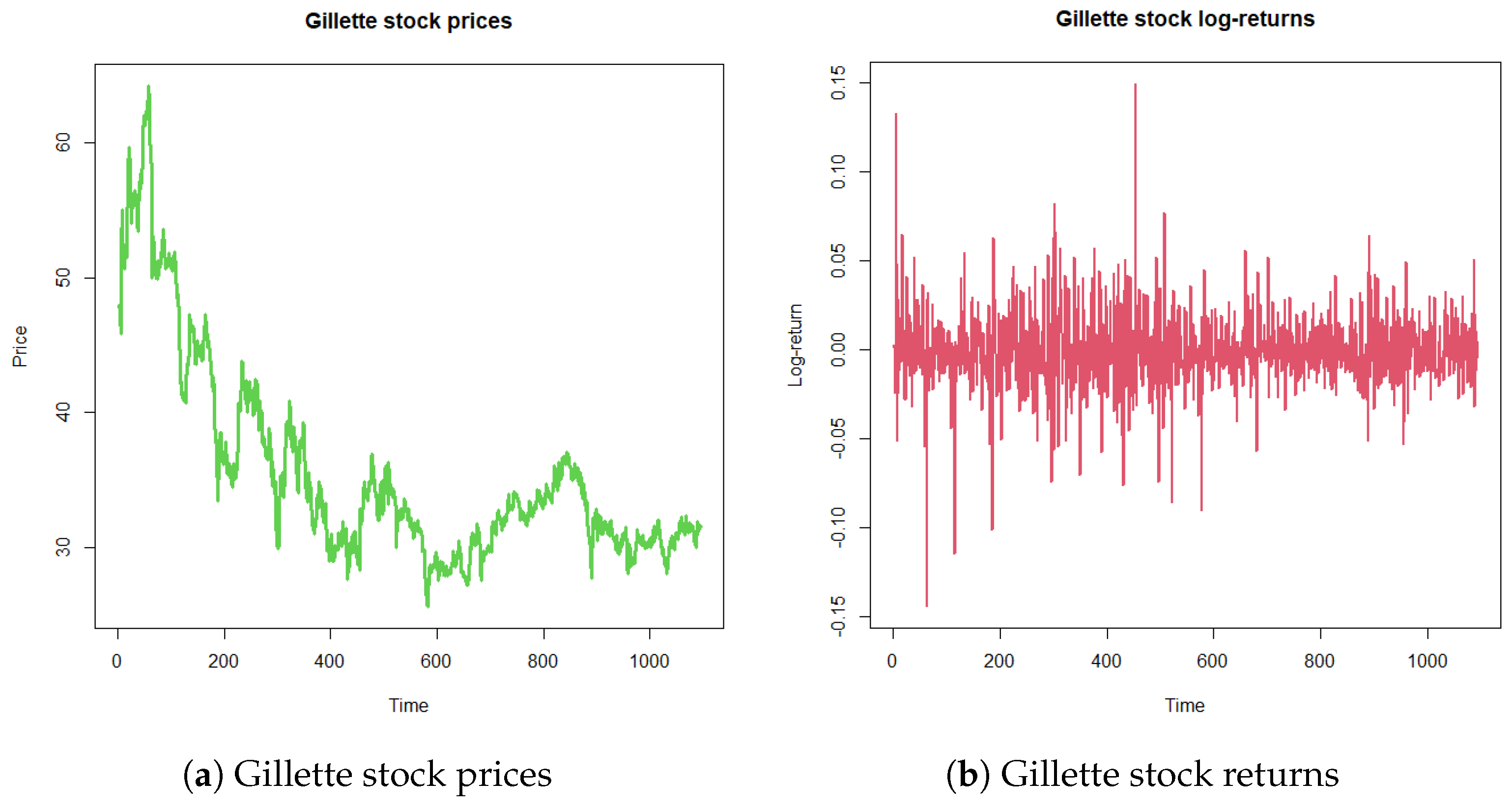
For a contrast with our theory, we study a time series dataset deeply studied in the time series literature. It considers the Gillette stock prices (, ) from 4 January 1999 to 13 May 2003 (Figure 1a). In terms of the continuously compounded return or logarithmic return, , Figure 1b exhibits the high volatility and conditional variance of the series. Despite the available models for volatility (ARCH, GARCH, TGARCH, EGARCH, etc.), a crucial hidden weakness of all time series estimation resides in the use of a likelihood based on an unrealistic independent probabilistic distribution sample. The underlying errors of the asset return models have been considered under different laws, such as Gaussian and generalized errors, among others. In this subsection, we consider the Kotz model of parameters, where , which contains the normal case, where .
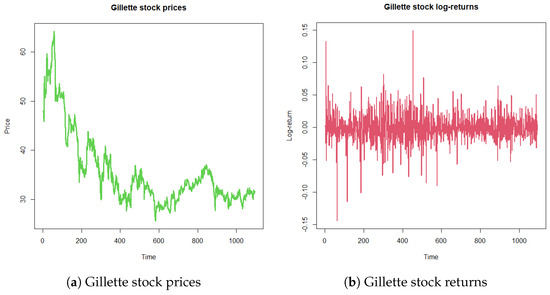
Figure 1.
Gillette stock time series from 4 January 1999 to 13 May 2003.
An optimization routine with the Optimx Package in Software R (4.1.1 version) provides the maximum log-likelihood estimation of the parameters. , , in the models ARCH(p), GARCH(p,q), TGARCH(p,q), and EGARCH(p,q).
The profile log-likelihood for the parameter Q in the ARCH() Kotz model is shown in Figure 2a, and the parallel behavior observed with the modified BIC criterion of Yang and Yang can be seen in Figure 2b.
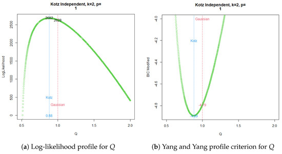
Figure 2.
ARCH Kotz independent ML estimation for .
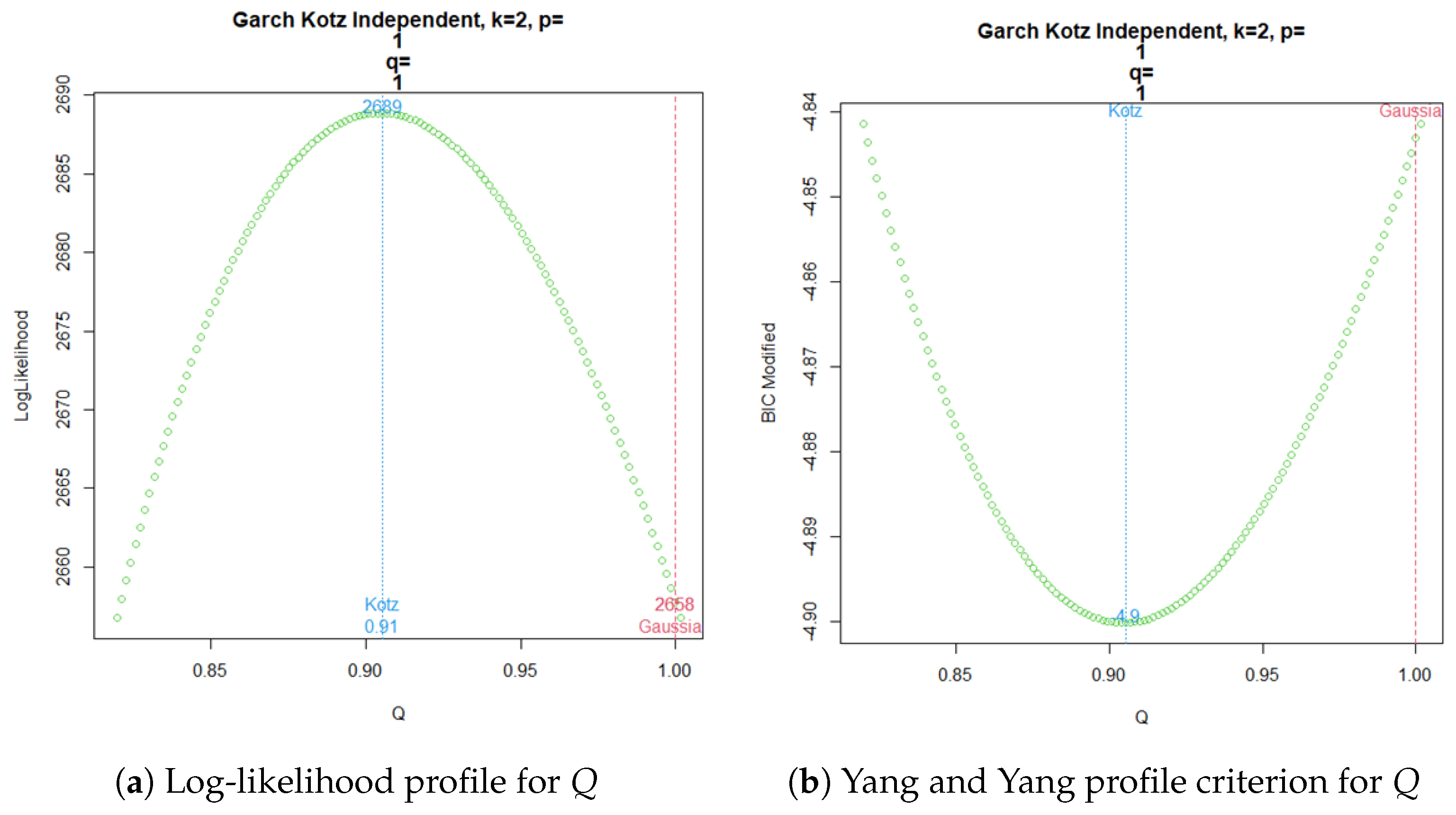
Figure 3a shows the profile log-likelihood for the parameter Q in the GARCH(, ) Kotz independent model. The corresponding modified BIC criterion from Yang and Yang for the profile behavior of Q is shown in Figure 3b.
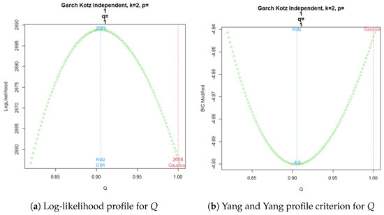
Figure 3.
GARCH Kotz Independent ML estimation for .
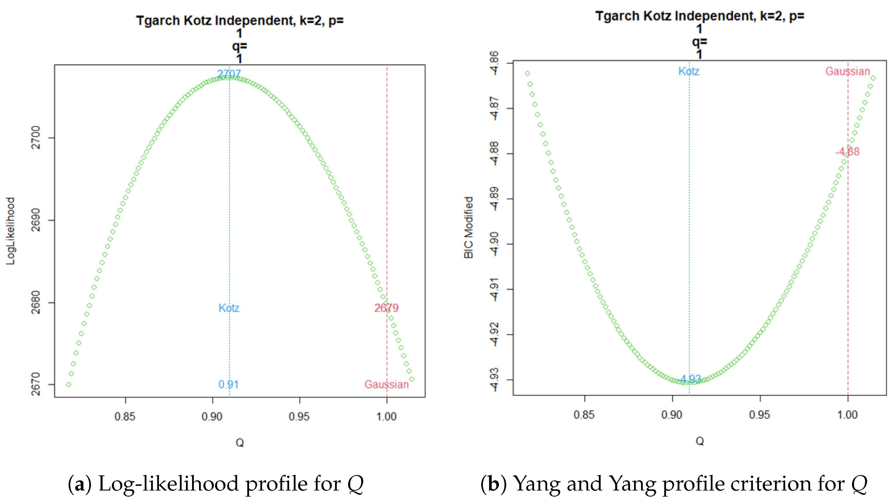
In a similar way, a TGARCH() Kotz model apparently favors a non-Gaussian model, as shown in Figure 4a for the log-likelihood profile of parameter Q. Meanwhile, Figure 4b exhibits the same conclusion from the modified BIC criterion proposed by Yang and Yang.
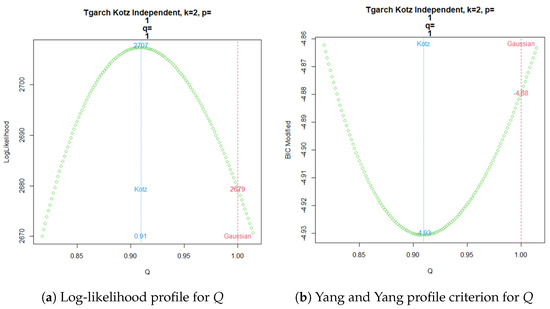
Figure 4.
TGARCH Kotz Independent ML estimation for .
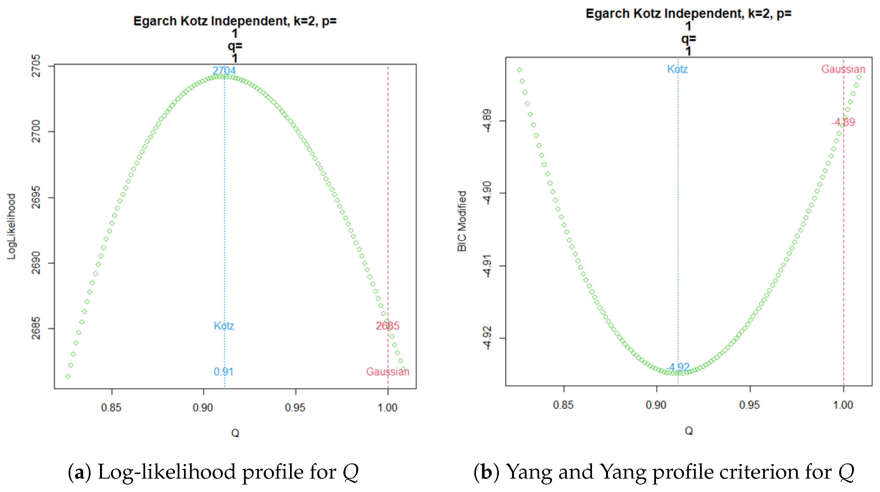
Finally, the EGARCH() for an independent Kotz model provides the log-likelihood profile of parameter Q in Figure 5a, which can be compared in parallel with the modified BIC criterion of Yang and Yang shown in Figure 5b.
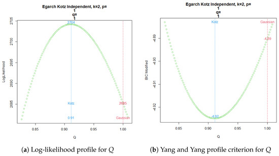
Figure 5.
EGARCH Kotz Independent ML estimation for .
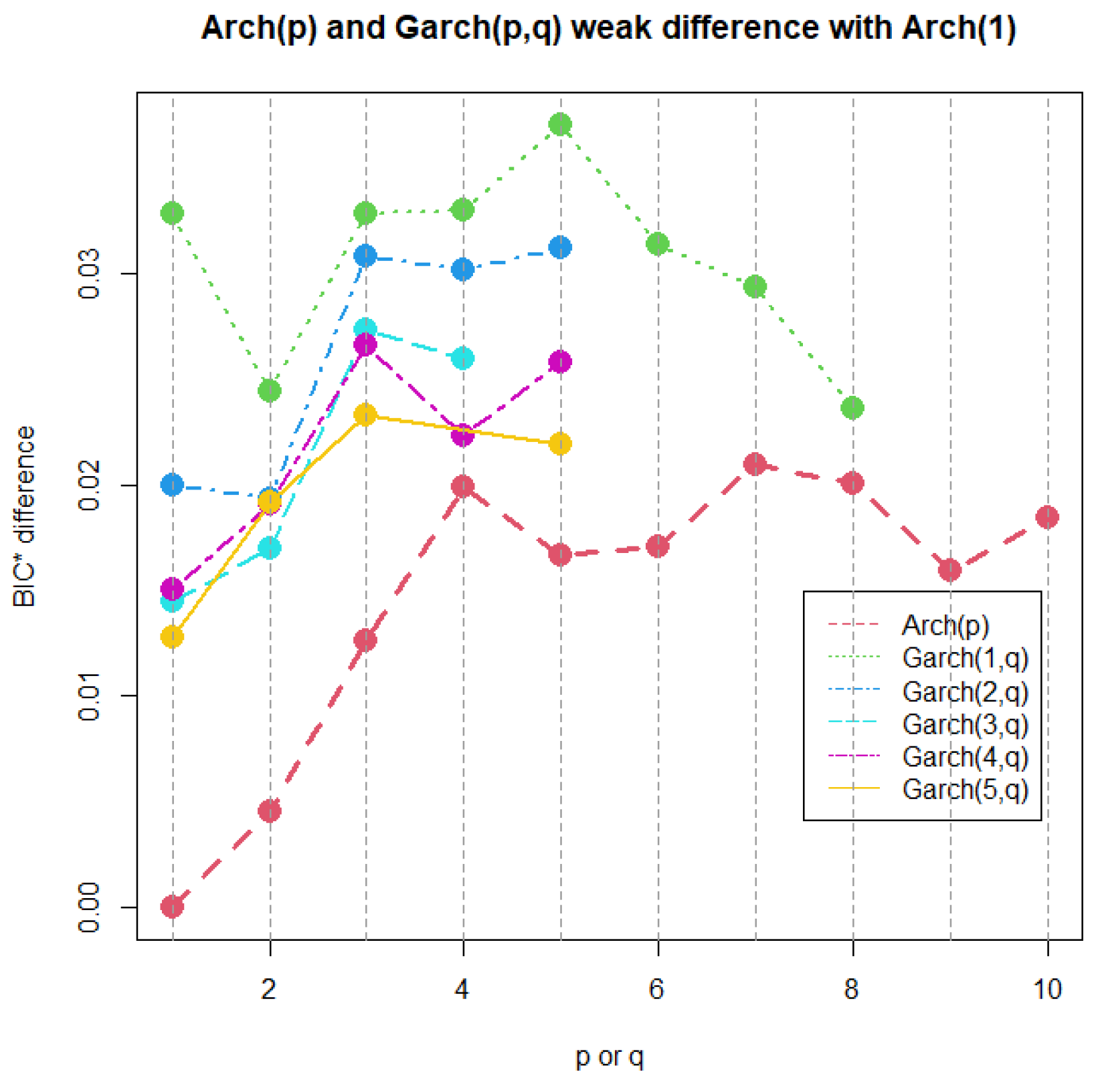
Now, a common practice since the emergence of time series volatility laws involves selecting the best model from two or more options using an information criterion. The AIC, BIC, and HQC are the classical decision criteria, and it can be seen in published real examples that preferences are based on minimal discrepancies. For example, in the current time series data, worldwide commercial software and papers have achieved the best model for extremely low differences around , without strong evidence of a meaningful difference. The models compared here are usually preferred in applications with increased complexity. In a Gaussian case, a GARCH model tends to be better than an ARCH model by several decimal points of BIC. However, GARCH performs worse with a similarly small BIC amount compared to TGARCH. Moreover, reports published elsewhere compared the latter models using BIC, without noting that they are not nested. Thus, here, we want to stress that each profile for Q is based on the new Yang and Yang criterion. C. C. Yang and Yang (2007). Figure 2b, Figure 3b, Figure 4b, and Figure 5b show that the respective Kotz model is better than the Gaussian case . It is not valid for this research that the apparently large differences in the Yang and Yang criterion of 0.1, 0.06, 0.05, and 0.03 determine a Kotz model of over a Gaussian model with , respectively; see Figure 2a, Figure 3a, Figure 4a, and Figure 5a. In order to solve a robust selection, we consider a comparison of the Yang and Yang criterion C. C. Yang and Yang (2007) with the modified BIC defined in (1). The corresponding comparison of the two models follows Kass and Raftery (1995) and Raftery (1995), with the evidence grades proposed in Table 1 for the BIC difference. Given that the ARCH(p) and GARCH(p,q) are nested models, we can compare them with a simple law. In this case, we find the BIC difference from the ARCH(1). The results for certain specific values of p and q can be found in Figure 6.
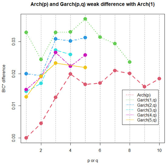
Figure 6.
ARCH(p) and GARCH(p,q) BIC difference with the ARCH(1).
A very weak difference in evidence between all models and ARCH(1) was obtained. No matter how complex the GARCH(p,q), the time series data cannot reach a plausible value near the minimum BIC difference of 2. In contrast, the classical literature would refer to GARCH(5,5) in this example as a more robust model than the simplest one, ARCH(1). The usual decision is based on the magnitude differences of in AIC, BIC, or HQC, but no evidence is provided from the studies investigated by Kass and Raftery (1995) and Raftery (1995). These data, which satisfied all the criteria for the analysis using ARCH and GARCH models, showed no notable enhancement in the complexity of the volatility representation. For this counterexample, the application of Kass and Raftery (1995) and Raftery (1995) in the time series setting raises an interesting question about the strong evidence of robustness in the variance models.
3.2. Application: Gillette Time Series Returns Under Dependent Probabilistic Samples Based on the Pearson Type VII Distribution
We devote a few lines to an application that considers the most important paradigm of this paper: the role of estimation in time series models with probabilistic independent samples, a fact that is regarded as the core of the likelihood itself. The likelihood has been viewed as an immutable concept in time series, but its philosophy clashes strongly with the natural concept of a correlated random variable fluctuating over time. No significant conceptual effort should be made to explain that time series are extremely correlated; therefore, their estimation, which is summarized in the likelihood, must consider dependent probabilistic samples. In this sense, the likelihood, reflecting the expected inner dynamics of the variable over time, naturally leads to a more realistic estimate of the volatility. This paradigm also appears in copula theory, which, in trying to solve the addressed evolution correlation, overlooks the underlying and hidden foundation of the likelihood and uses it for parameter estimation, straying from the original intention of avoiding independence. Thus, implementing a new perspective on the likelihood of a vector variate that is strongly dependent on time should address the problem of volatility. We have observed the aforementioned effect in similar stages of financial models. This was the case in Díaz-García et al. (2022), where a classical likelihood decision based on the mean of a bivariate distribution was situated at the tails of the right distribution estimated by a probabilistic dependent likelihood.
Considering, again, Gillette’s time series returns, if we provide a Pearson Type VII model for the underlying errors indexed by the non-estimated degrees of freedom r, then a plausible likelihood emerges in (7). Inspired by the problem of very weak evidence for this special set of returns, and for the sake of illustration, we estimated the simplest models of volatility: ARCH(1), GARCH(1,1), TGARCH(1,1), and EGARCH(1,1). As in the independent case, we used several methods of optimization, supported by gradients and Hessians. All of them converged to the same estimation. Table 2 provides the results of each model and the corresponding comparison with the BIC criterion for ARCH and GARCH, along with the following CAIC criterion for the remaining nested models (Bozdogan, 1987).
where is the maximum log-likelihood, n is the sample size, and is the number of estimated parameters.
Table 2.
Comparison of independent and dependent models.
Table 2 refers to the comparison of Kotz TGARCH(1,1) and Kotz EGARCH(1,1) with the simplest model, Kotz ARCH(1), for independent probabilistic samples. Given that the three models are not nested, we can only use the CAIC difference; however, no evidential criteria for those magnitudes are available. This implies that no conclusion can be drawn about the best model. The usual selection in favor of the best difference does not hold, i.e., we cannot affirm that Kotz TGARCH(1,1) is the best model. A similar non-nested comparison is achieved in the dependent case for Pearson EGARCH(1,1) and Pearson TGARCH(1,1); that is, we cannot guarantee that the CAIC difference of 0.062476 defines the Pearson TGARCH(1,1) model across the remaining two laws. However, when the models are nested, we can use Kass and Raftery (1995) and Raftery (1995) as evidence of the BIC difference. This is the case for Table 2, where Pearson GARCH(1,1) and Pearson ARCH(2) with degrees of freedom are compared to the simplest model, Pearson ARCH(2) with 1 degree of freedom. Notably weak evidence was obtained, and the BIC differences were well below the 2 limit, for a positive predominance of GARCH(1,1). Therefore, the five models referred to, with increased complexity, did not achieve a better performance than the simplest Pearson ARCH(2). In this sense, the limits of the rigorous evidence for the best model, according to Kass and Raftery (1995) and Raftery (1995), open an interesting avenue for future work on this example. Moreover, a further study of Kass and Raftery (1995) and Raftery (1995) in the setting of non-nested models via CAIC should provide similar bounds of significant evidence. This important issue will be part of future work.
3.3. Gross Domestic Product (GDP)
Defense spending as a proportion of GDP, analyzed quarterly, can fluctuate over time due to economic, political, and geopolitical factors. ARCH models are particularly useful for studying this conditional heteroskedasticity, which refers to time-dependent changes in variance.
In economic contexts, defense spending volatility is often influenced by events such as armed conflicts, economic crises, or shifts in fiscal policy. Modeling this series using ARCH allows examining how past shocks affect future variability, providing deeper insights into the risks associated with this type of spending.
Fluctuations in defense spending relative to GDP can have significant impacts on macroeconomic stability. For instance, an unexpected increase in this spending could divert resources from other critical sectors, negatively affecting overall economic growth. ARCH models assist in quantifying and analyzing these fluctuations, enabling a more accurate assessment of their potential effects.
Recent studies have applied ARCH family models to analyze GDP in various countries, offering valuable perspectives on volatility dynamics and their economic implications. Datta Gupta et al. (2023), Muma and Karoki (2022), Ma (2024) and Miladinov (2021).
The analysis carried out on Gillette’s share returns showed weakness in the evidence of differences for all simple and complex models considered. However, it is interesting to observe whether this trend is present in other sectors, such as macroeconomics. We considered the GDP time series, which is sufficiently broad across historical moments in recent modernity, it is also unique, given the wide range under consideration, from Q1 1947 to Q3 2024. This allows users to see how the percentage of GDP allocated to national defense has changed over time. We will observe whether the classical approximation of a likelihood based on independent samples (5) manages to detect any evidence greater than weak.
In this analysis, we also include a novelty that allows comparisons to be made using known results that relate the Pearson VII elliptic model and its degrees of freedom with their asymptoticity, which, both in probability and distribution, converge to the Gaussian case when such a parameter tends to infinity.
Since the t-distribution, a particular case of the Pearson VII elliptic model, is available in most free and commercial software, we use calculations and the expected Gaussian convergence to calibrate its accuracy. As we will see in Section 4, using one of the most well-known commercial time series software packages showed certain inconsistencies with expected results.
However, the results were valid for approximate magnitudes of and made decisions based on significant evidence.
For a first approximation of the effect of the degrees of Freedom in the four models, we initially considered the following degrees of freedom . Then, in each model and according to the maximum number of degrees of freedom supported by the commercial software in each case, we performed a search for the degree of freedom that supported the most information for the criterion. Its left and right neighbors were also indicated, as well as the calculation of the highest permissible degree of freedom. Finally, the expected asymptotic result of the Gaussian case was also indicated.
Table 3 shows the results for the ARCH(1), ARCH(2), GARCH(1,1), TGARCH(1,1), and EGARCH(1,1) models.
Table 3.
Comparison of models of GDP time series for the independent case. Each block includes the best degree of freedom as the reference model with maximal information; then, the corresponding nested BIC difference is computed with the remaining degrees of freedom and the Gaussian limit. All possible pairs show weak BIC evidence. Moreover, the nested comparison of GARCH and ARCH also exhibits weak BIC evidence. For the non-nested models via CAIC, the reference corresponds to the simplest ARCH(1) supported by a Gaussian distribution, and a corresponding very low difference was computed. Negative differences mean that the low dominance is inverted in the specific pair under consideration.
In each model, the greatest amount of information was observed in the criteria of degrees of freedom accompanied by the label best. The best degrees of freedom were achieved in 3, 4, and 5, while the maximum values allowed by the commercial software were relaxed to fit the respective normal models, as expected.
This asymptotic behavior, known only at a distributional and probabilistic theory level, seems to be confirmed in the information on the criteria, an aspect that can, in turn, be constituted as a heuristic method for verifying convergence and obtaining global minima. This aspect will be studied in the future.
However, for the purposes of this article, we note that the comparisons of all nested models, without exception, involved weak evidence. The CAIC differences between non-nested models are also presented; however, interpreting them requires a more theoretical background. A heuristic method is discussed in Section 4.
The macroeconometric GDP series is crucial in time series analysis, as it utilizes aggregate data to estimate fiscal shocks (Ramey, 2011; Gurgel-Silva, 2021). Similarly, aggregate data have been employed to assess the impacts of government spending on corporate profits (Cortes et al., 2024). The seasonality of macroeconometric time series is important for extracting a substantial amount of information, but it is affected by volatility; hence, studies examining criterion differences are essential. In this research, the GDP results indicate that all models and studies produced weak evidence. This outcome aligns with expectations, especially since samples were collected quarterly, which smooths the variance and conceals the strong daily volatilities in the Gillette and S&P 500 series. The framework presented in this article addresses the significant need for evidence regarding the differences between the two models and encourages future research. Even the daily time series examined here, which demonstrated considerable volatility, showed negligible differences for complex models such as EGARCH and TGARCH, in both dependent and independent observations cases.
There was consistency in all the examples studied here, from various perspectives (macroeconomics, microeconomics, dependence, independence, ARCH, GARCH, TGARCH, EGARCH models, nested, and non-nested). This suggests an additional study for time series users related to significant evidence of differences between two models. The theorems established in Section 3 indicate a paradigm shift, as they highlight transitional relationships between criteria and the translation of evidence. Although this article aimed to create a unified theory based on theorems that do not rely on either the macro or micro econometric sector, it is noted that all the examples studied revealed a weakness in the evidence. This should prompt future work on developing different volatility models that clearly identify significant differences in the information that promotes the likelihood.
In particular, we anticipate volatility models that can amplify or reduce the length of the intervals of evidence of differences, such that one criterion is not a simple translation of another. According to the theorems in Section 4, currently, the information criteria inherit by simple translation the evidence of the simplest model. Computationally, this is an advantage, since heuristically it is sufficient to perform an initial study of the simplest ARCH(1) model and its convergence in probability with Pearson VII type errors, parameterized with their degrees of freedom towards the Gaussian model. But the problem emerges in the transitions of the differences for more complex models, when evidence greater than weak is reached, given that all intervals have the same length, regardless of the selected criterion. This new problem raises the following question: Is there a criterion based on likelihood that is not invariant in translation to the classical criteria? Or will all information criteria always be invariant under evidence translation and therefore have a unique pairwise transition number, in the sense of the results established in Section 4? The answer to these questions could help in differentiating the true role of time series models and their relationship with the information criteria for their selection.
3.4. Application: The S&P 500 Index
The S&P 500 index, one of the main benchmarks for the stock market in the United States and internationally, comprises the shares of 500 large U.S. companies and serves as a key indicator of the overall performance of the country’s stock market. At the onset of the COVID-19 pandemic, the S&P 500 experienced a sharp decline of nearly 40%, but it recovered in less than six months, reaching and even surpassing pre-crisis levels. This phenomenon highlights investor expectations in financial markets and the impact of the Federal Reserve’s expansive monetary policies.
The composition of the index is subject to a periodic review to align with market dynamics. Companies are added or removed based on market capitalization and other relevant criteria, with revisions typically occurring every quarter; however, adjustments may occur more frequently in response to significant market events. Furthermore, recent analyses of the S&P 500, utilizing ARCH family models, have been used to assess its behavior and the prevailing trends (Al-Momani & Dawod, 2022, Belhachemi, 2024, Vo & Ślepaczuk, 2022, Yilmazkuday, 2021).
We repeated the same analysis as for the GDP data by taking advantage of the limiting behavior in the Pearson VII model. Again, the same weak evidence was obtained for all the possible pairs under consideration. The results are shown in Table 4.
Table 4.
Evidence for differences among the models of the S&P 500 data under the independent setting.
As before, the maximal information criteria were obtained at low degrees of freedom; thus, this reference model governed a very weak difference with the remaining parameters until the greatest admissible parameter for the commercial software approached the Gaussian limit. For nested models, the BIC difference was computed with the remaining degrees of freedom and the Gaussian limit. All possible pairs showed weak BIC evidence. The nested comparison of GARCH and ARCH also provided weak BIC evidence. For the non-nested models via CAIC, the reference corresponded to the simplest ARCH(1) supported by a Gaussian law, and the corresponding very low difference was computed. For these data, no negative CAIC differences were obtained in favor of the Gaussian model, but an evidence classification could not be provided.
Up to this point, we have studied the independent case and observed repetitive weak evidence for all pairs of models considered, regardless of their hierarchy and theoretical robustness. What is valuable comes from maintaining the criteria of the well-known convergences in probability and distribution emerging from the Pearson VII model. This suggests an analysis with more degrees of freedom that covers the largest possible domain. We studied this technique for the dependent case. Its significance necessitates a dedicated section.
4. Discussion
In this section, we apply the process of analytical induction to create general relationships that emerge from the particular cases studied in Section 3. Specifically, the S&P 500 time series under the simple ARCH(1) model and its counterpart, the much more complex EGARCH(1,1) model, revealed a unique result.
4.1. Discussion Part 1
Table 5 compares the criteria for each of the two models evaluated on the same S&P 500 time series. The upper triangular table shows the differences between all criteria for the ARCH(1) model. The lower triangular table focuses on the EGARCH(1,1) model, showing all possible pairs of differences between the same criteria.
Table 5.
Additive constants for the criteria equivalence of nested ARCH(1) (upper triangular) and EGARCH(1,1) (lower triangular).
Initially, let us consider the upper triangular table. The value represents the AIC–BIC difference. If the model is evaluated with a single degree of freedom for the Pearson VII distribution, then the value is not of interest. However, in the modeling carried out, a wide range of degrees of freedom was considered, ranging from 1 to , so that the model was examined across its full complexity, up to the normal limit expected for large degrees. The fact that AIC-BIC = was valid for each of the ARCH(1) models with such dissimilar degrees of freedom is of interest, since it was a notable constant, independent of the important shape parameter in t-distribution. Specifically, the constant difference was maintained for the following degrees of freedom: 1, 2, 3, 4, 5, 6, 7, 8, 9, 10, 20, 30, 40, 50, 60, 70, 80, 90, 100, 200, 300, 400, 500, 600, 700, 800, 900, 1000, 2000, 3000, 4000, 5000, 6000, 7000, 8000, 9000, 10,000, , , , , , , , , , . This means that the difference between any pair of criteria was invariant under the considered degrees of freedom.
Now, if the subindex stands for AIC, BIC, HQC, BIC, and CAIC, respectively, then = criterion-criterion in the ARCH(1) model and = criterion-criterion for the EGARCH(1,1) model. For example, for the ARCH(1) model, the upper triangular constants read In the EGARCH(1,1) model, the lower triangular additive constants for the CAIC mean that
The additive constants in this example seem new in time series applications and information theory. A general mathematical expression is not straightforwardly obtained from the implied definitions; otherwise, the development of such a theory could have been simplified over the years. However, in the current time series example, a simplification, indeed, appears.
4.2. Discussion Part 2
Applying the correct settings, a general formula can be derived based on the findings from the initial part of Section 4.1.
Given that the criteria are applied to the same model and data, the maximum log-likelihood holds for all of them. The definition of the criteria studied is easily described by the constant term , namely:
Then, any criterion can be expressed as
Moreover, the function is linear in , then
Finally, any difference between two criteria takes the general form:
where the particular functions of the sample size n are given by
And now we can obtain any criterion for particular data. For the upper triangular Table 5, the ARCH(1) model involves parameters and a time series of . Then, . Similarly, the remaining differences can be obtained from the upper triangular table.
For example, since the CAIC criterion is usually for non-nested models, we provide the following simple equivalences for the S&P 500 log returns in the dependence case:
For the EGARCH(1,1) model of the lower triangular table, the only change involves two more parameters than the ARCH (1) model, i.e., , then , and the other coefficients for the EGARCH(1,1) model can be obtained.
At this stage, we have exact formulae for any difference between two criteria applied to the same model, and then the upper and lower triangular in Table 5 can be constructed separately. However, the differences for the complex model seem to reflect an additional property. The lower triangular table is written in terms of the results for the simplest model, ARCH(1). Numerically, there is a constant, 1.4, that appears in any difference and expresses the difference of the criteria in EGARCH (1,1) in terms of the corresponding difference in ARCH(1).
The example of the CAIC criterion in the EGARCH(1,1) model implies the following simple equivalences.
The novelty of additive constants thus faded when we found that a more general constant could be established for these particular data. The dilatation constant 1.4 holds for all relations in the lower triangular equalities. Given its importance, this dilatation constant will be referred to as the transition number for nested ARCH(1) and EGARCH(1,1) models.
This means that, for the data considered, any criterion for the simplest model ARCH(1) can be explained exactly (with an accuracy of six decimal places) by the behavior of the criterion of the complex model EGARCH(1,1). The relationship is simply a shift and dilation of the models.
This intriguing relationship presents a formula for consideration that is quite straightforward.
Let and be the number of parameters in the upper and lower models, respectively. For the upper triangular relation , meanwhile, for the lower triangular equivalence.
Then,
and
Thus,
for all . Next, we can easily find the transition number between the complex lower model by referring to the parameters in both models we are looking at.
In Table 5, the behavior of the lower triangle table with the more complex EGARCH(1,1) model can be predicted using the simplest model in this paper, ARCH(1). In this case, the transition number takes the form:
for all .
We recall that each EGARCH(1,1) model for the dependent case was calculated using a total of 47 degrees of freedom from 1 to , and the calculations for each were optimized through various methods available in the Optimx R package. Each calculation was performed exhaustively until all available methods converged to the same value, with a resolution of six decimal places. On a personal computer, this task takes days, while calculating the simplest model, ARCH(1), is much quicker. The transition relation found proposes a method of analysis in time series that only requires the calculation of the simplest model; and with it, any of the more complex models, such as GARCH, TGARCH, and EGARCH, can be predicted.
The method is also interesting from an optimization point of view, as it is consistent with the calculations in commercial software. It is expected that for the same time series, the models studied here comply with the transition constant up to a certain number of decimal places. If the results of the more complex model are not derived from the simpler model with a tolerance similar to the one used in this example, which is , then the optimization algorithm is neither sufficiently stable nor reliable. The tables of the independent case were created using well-known commercial software. As expected, the transition constants are not the same in the tolerance of six decimal places, see Table 6.
Table 6.
Additive constants for the criteria equivalence of nested ARCH(1) (upper triangular) and EGARCH(1,1) (lower triangular) for the independent case, computed with a well-known commercial software. The constant 1.4 was not reached for all the differences in the lower triangular table.
In summary, a critical area remains to be investigated. If the most basic model, ARCH(1), can predict the distinctions among the criteria of all the models analyzed here, what role do the more complex models play in this scenario?
This indicates that we need to quantify the importance of the difference between two given criteria for a pair of models: one complex and one simple.
Table 5 allows for differences between the criteria for the same model, but our interest now lies in comparing the more complex model with the larger model.
We now ask whether the difference between the two models applied to the same time series is significant enough to choose the more complex model. If so, should all the expensive computational calculations be performed instead of simply computing the smaller model?
In the classical literature, it is common to choose the best model that meets the lowest criterion. In some cases a choice of minimal discrepancies of in criteria is achieved. It seems to be a widespread practice that the most complex models tend to have more information on likelihood and, therefore, exceed, as expected, the smaller models; thus, the most complex ones are generally chosen.
This answer is well known in other areas of classical statistics, but it seems to be less well established in time series. The choice of the best model is left to a process of elementary measurability, regardless of the order of the differences. Raftery found the answer more than 30 years ago through the so-called weak, positive, strong, and very strong difference evidence.
Using Bayesian theory, he established approximate limits for the difference in the BIC between two models. That classification is so demanding that, for barely acceptable evidence, referred to as positive, a difference greater than approximately 2 is required; otherwise, it is insignificant, and the best model must be the simplest one. Thus, in this case, the large expense spent on the more complex model was unnecessary. Assume weak evidence; this means that
The above results on additive constants and transition numbers allow general formulas for checking evidence between non-Bayesian criteria. In particular, we study again the simplest criterion, the AIC.
To achieve this, we act on the above inequality using the general additive constants that were previously derived.
Let and denote the BIC and AIC for Model 1 with the parameters . Similarly, and are the BIC and AIC for Model 2 with parameters . Then, the Strong evidence for BIC can easily be mapped to the Strong evidence for AIC. Starting with
The additive constant for BIC and AIC adjusts the inequality as
And, finally, the weak evidence for the AIC difference between the two models is given by
The remaining intervals for weak, strong, and very strong differences in AIC can be easily mapped; the AIC evidence is condensed into the following Table 7.
Table 7.
Grades of evidence for AIC difference.
The lower bound of the weak evidence can be zero, allowing a model to be perfectly similar to itself. However, such a bound is irrelevant, since, in any case, the result indicates weakness in comparing the more complex model with itself and, therefore, recommends the simpler model.
At this point, we can answer the question inherent to the transition from the simple ARCH(1) model to the more complex EGARCH(1,1) and its high computational cost. The shift parameter in this case is given by
Thus, strong evidence is located in the interval .
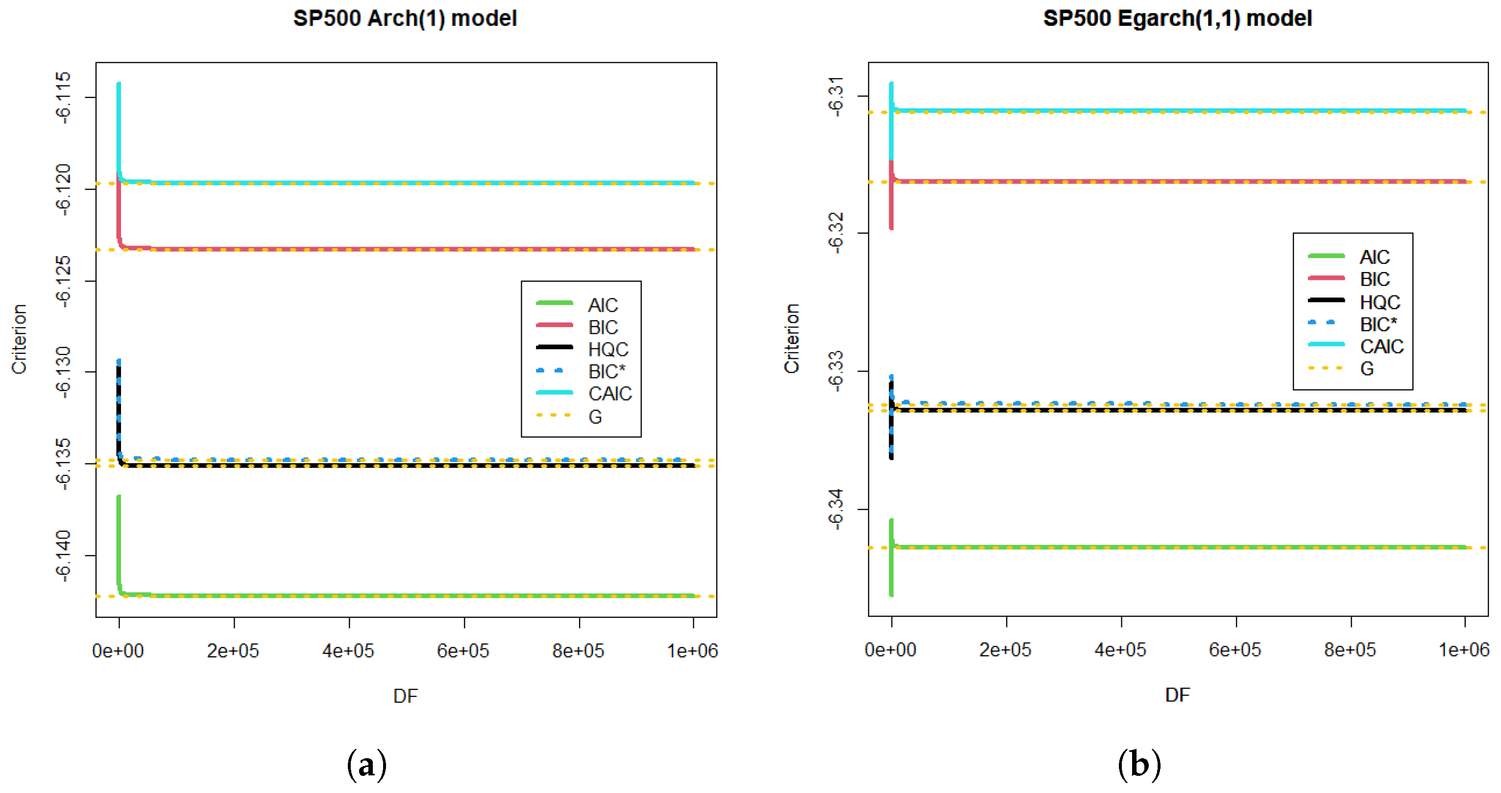
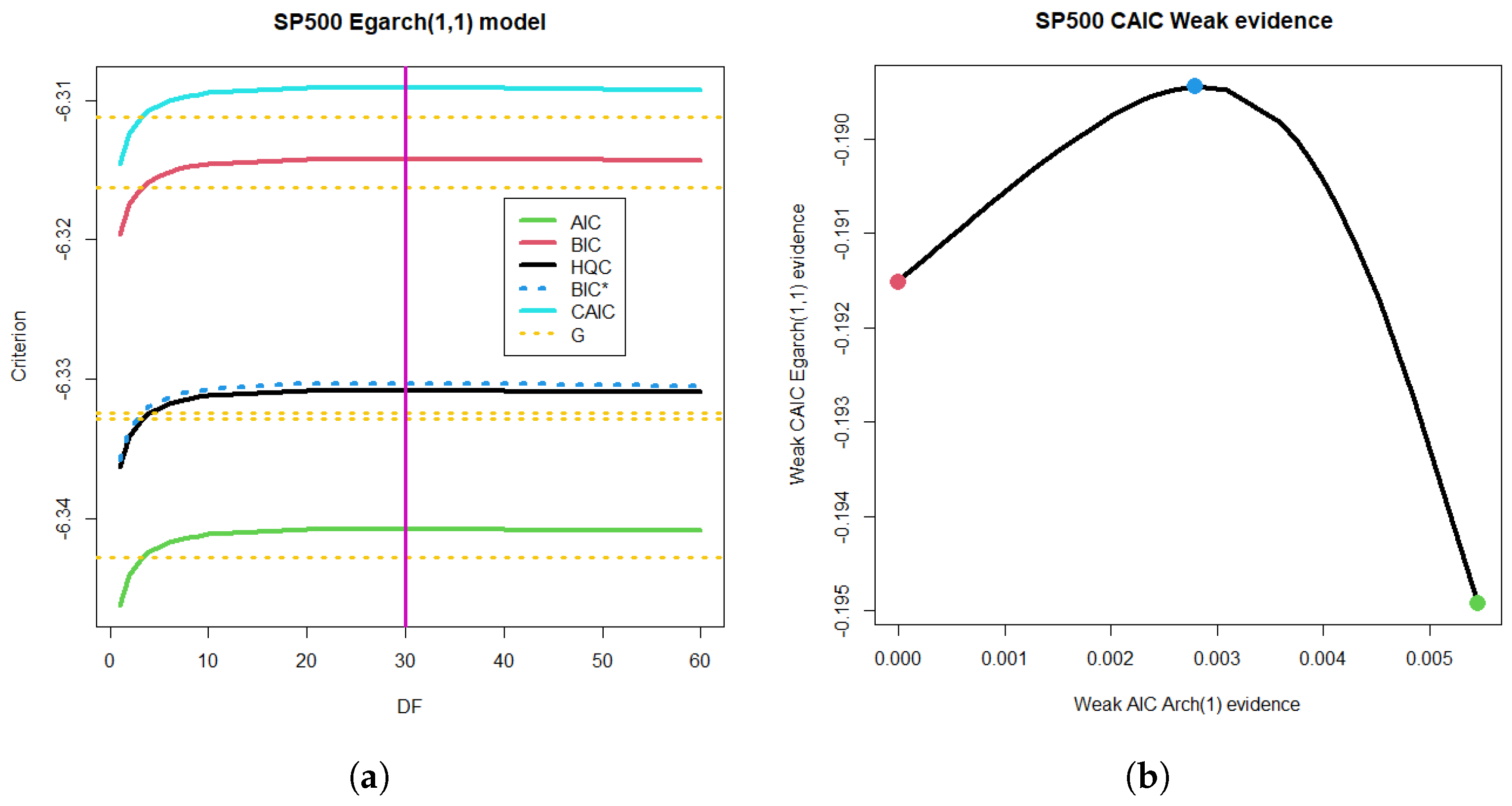
For comparison purposes, let us consider the ARCH(1) model with the reported degrees of freedom (see Figure 7a). For a million degrees of freedom, each criterion brings it closer in probability to the Gaussian model (see the yellow limit of Gaussian estimation for each criterion in Figure 7a). Let us take EGARCH(1,1) as the most complex model, with a great computational cost to achieve the required accuracy in the transition number to the simple ARCH(1). If we calculate the differences in the AIC criterion for the most complex model with all the degrees of freedom studied (from 1 to ), we obtain Figure 7b with the corresponding Gaussian limit (yellow).
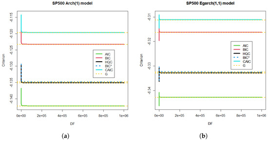
Figure 7.
ARCH(1) and EGARCH(1,1) models for S&P 500 time series for the dependent case. (a) Criteria for S&P 500 time series in the dependent case and the ARCH(1) model. The Gaussian limit G is also depicted for the limit of each criterion. The degrees of freedom (DF) were studied from 1 to . (b) EGARCH(1,1) model and criteria for S&P 500 time series in the dependent case. The Gaussian limit G is also shown.
The ARCH(1) model exhibited a monotonic decreasing relation with the degrees of freedom DF. Meanwhile, the EGARCH (1,1) model showed a one-mode behavior with a maximum at and a Gaussian limit tendency for large DF; see Figure 7.
In the criterion subindex notation of this section, if we denote as the shift in BIC evidence for any criterion j, including BIC (), the Table 7 is easily written for any reference. However, in this work, we prefer to set the AIC evidence intervals and the ARCH(1) model as global references, given their simplicity.
A similar analysis of the remaining criteria led to a corresponding evidence table for AIC indexed by a different shift constant for the BIC intervals. Furthermore, due to its interval translation character, the interval was neither widened nor narrowed, so the Raftery evidence indicator for BIC had the same amplitudes for the other criteria: Weak, 2 units; Positive, 4 units; Strong, 4 units.
We conclude this section with a discussion of the complex problem of comparing non-nested models. This problem is outside the scope of this paper, but we provide a brief discussion of the implemented models. Once we have calculated the simplest criterion and have its evidence across a whole range of degrees of freedom, we can expect a relationship with the CAIC criterion suitable for non-nested models. Specifically, we are interested in mapping the weak evidence of the ARCH(1) model, parameterized by its degrees of freedom, to the CAIC differences of the EGARCH(1,1) model with the same degrees of freedom. In this case, the target model was ARCH(1) with 1 million degrees of freedom, and the remaining 46 models were compared simultaneously with the same reference.
The heuristic method we propose is based on using a Pearson-type model and sweeping the entire domain of degrees of freedom to implement convergence in probability toward the normal. Although the mapping is performed via likelihood, this convergence is not guaranteed; however, it limits the relationship between the differences in the CAIC and the differences in the ARCH. The ARCH(1) model is the independent variable in the example we are considering, because it is much simpler. It has the particularity of following a decreasing monotonicity in the degrees of freedom, while the EGARCH(1,1) that we have considered exhibits unimodal behavior. Thus, the range of the expected function is limited by the function’s boundaries at 1 and degrees of freedom. The monotonicity also ensured that the maximum of 30 degrees was mapped to the maximum in the estimated model. The result can be seen in Figure 8b. This nonlinear relationship doubled the ideal segment of linear mapping between ARCH(1) and EGARCH(1,1) for the case of the same criterion, resulting in evidence that, in absolute value, is certainly weak.
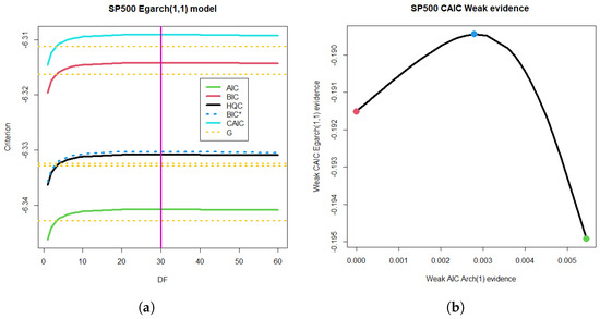
Figure 8.
Mapping weak differences from the ARCH(1) model to the non-nested EGARCH(1,1) model and their CAIC differences. (a) One-mode tendency of the EGARCH(1,1) model with mode in 30 degrees of freedom and decreasing limit to the Gaussian criteria of Figure 7. (b) Heuristic method for non nested comparison between EGARCH(1,1) and ARCH(1) models.
5. Conclusions
The paper proposed a so-called dependent time series from a new perspective of likelihood based on dependent probabilistic samples governed by a general class of distributions that also allow multiple forms of volatility. The article also included robust selection criteria for classic volatility models and required degrees of evidence to differentiate the modified BIC criterion from other areas.
Degrees of evidence that progress from weak to very strong leave no room for significant differences in a well-established time series. These are typically addressed using hierarchical models, which assign a better explanation to more complex models. However, with the introduction of the new evidence scale, they failed to achieve even the minimum difference with the simplest model. One notable example was the case of macroeconomic data, where the family of models designed for volatility was expected to exhibit a weak fit. It is important to note that if the model shows a weak fit with the simplest model, this weakness also applies to the more complex models.
This paradigm of dependent time series, generalized under families of distributions and hierarchized by demanding degrees of evidence, consolidates an alternative to artificial intelligence approaches and other increasingly complex volatility models. However, it encounters the same difficulties with activation functions and in differentiating the effect of volatility. Finally, given the small sample and nonseasonal events that strongly affect the foundations of classical volatility models, there are parallels to study in the future, and to relate the new view of likelihood presented here to volatility modeled using the recent spectroscopic shape theory by Villarreal-Rios et al. (2019).
The findings of this paper, if we want to enumerate them, are the following:
- Dependent time series errors under elliptically countered models.
- Independent time series errors under elliptically contoured models.
- Time series classification for volatility models via evidence of differences in a modified BIC decision criterion.
- Definition of ARCH(p), GARCH(p,q), TGARCH(p,q), and EGARCH(p,q) volatility time series models in the context of dependent time series errors under elliptically countered models.
- Definition of volatility time series models of ARCH(p), GARCH(p,q), TGARCH(p,q), and EGARCH(p,q) in the context of independent time series errors under elliptically contoured models.
- Explicit formulas for a general class of independent probabilistic samples derived from the Kotz distribution.
- Explicit formulas for the general class of dependent probabilistic samples based on the Pearson Type VII distribution.
- Exact formulas for comparing criteria among AIC, BIC, HQC, BIC, and CAIC.
- Exact formulas for general transition numbers among the following criteria: AIC, BIC, HQC, BIC, and CAIC.
- New general setting for comparison of criterions using difference evidence, applied to AIC, BIC, HQC, BIC, and CAIC.
- Heuristic approach for comparing two non-nested models.
- A computational comparison between worldwide commercial software for a particular model in the independence case and the algorithms developed from the general theorems here derived.
- Full detailed examples for micro and macro economic sectors include Gillette and SP&500 returns, as well as Gross Domestic Product.
- Proposition of a heuristic method for computational calibration based on the probabilistic convergence of the Pearson type VII model to Gaussian law.
Author Contributions
Conceptualization, J.A.D.-G.; Methodology, F.O.P.-R.; Validation, F.O.P.-R.; Formal analysis, F.J.C.-L.; Investigation, G.G.F. All authors have read and agreed to the published version of the manuscript.
Funding
This research received internal funding of University of Medellin.
Data Availability Statement
No own data was generated for this research.
Acknowledgments
We thank the referees for their comments and suggestions to improve this work. The author F.O.P. thanks the Ph.D. in Modeling and Scientific Computing Program and the High-Level Education Committee of the University of Medellin for supporting his doctoral studies. G.G.F. gives thanks for the partial support PID2023-147593 NB-I00, Ministry of Science, Research, and Universities, Spain. The authors express their gratitude to Miguel Bedolla for his revisions to the manuscript.
Conflicts of Interest
The Authors declare no conflicts of interest.
References
- Al-Momani, M., & Dawod, A. B. (2022). Model selection and post selection to improve the estimation of the ARCH model. Journal of Risk and Financial Management, 15(4), 174. [Google Scholar] [CrossRef]
- Baillie, R. T., Bollerslev, T., & Mikkelsen, H. O. (1996). Fractionally integrated generalized autoregressive conditional heteroskedasticity. Journal of Econometrics, 74(1), 3–30. [Google Scholar] [CrossRef]
- Belhachemi, R. (2024). Hidden truncation model with heteroskedasticity: S&P 500 index returns reexamined. Studies in Economics and Finance, 41(5), 1085–1105. [Google Scholar] [CrossRef]
- Bollerslev, T. (1986). Generalized autoregressive conditional heterocedasticity. Journal of Econometrics, 31, 307–327. [Google Scholar] [CrossRef]
- Bozdogan, H. (1987). Model selection and akaike’s information criterion (AIC): The general theory and its analytical extensions. Psychometrika, 52, 345–370. [Google Scholar] [CrossRef]
- Cai, G., & Wu, Z. (2022). Construction of functional EGARCH model and its volatility prediction. Statistical Research, 39(5), 146–160. [Google Scholar]
- Chaudhary, R., Bakhshi, P., & Gupta, H. (2020). Volatility in international stock markets: An empirical study during COVID-19. Journal of Risk and Financial Management, 13, 208. [Google Scholar] [CrossRef]
- Chen, J., & Politis, D. N. (2019). Optimal multi-step-ahead prediction of ARCH/GARCH models and NoVaS transformation. Econometrics, 7(3), 34. [Google Scholar] [CrossRef]
- Chu, J., Chan, S., Nadarajah, S., & Osterrieder, J. (2017). GARCH modelling of cryptocurrencies. Journal of Risk and Financial Management, 10, 17. [Google Scholar] [CrossRef]
- Cortes, G., Vossmeyer, A., & Weidenmier, M. (2024). Stock volatility and the war puzzle: The military demand channel. Nber Working Paper Series, Working Paper 29837. National Bureau of Economic Research. Available online: https://www.nber.org/papers/w29837 (accessed on 27 February 2025). [CrossRef]
- Datta Gupta, M., Rahman, M. M., Sultana, Z., & Rahman, F. M. A. (2023). An ARCH volatility analysis of real GDP, real gross capital formation, and foreign direct investment in Bangladesh. Asian Economic and Financial Review, 13(4), 228–240. [Google Scholar] [CrossRef]
- Ding, Z., Granger, C. W. J., & Engle, R. F. (1993). A long memory property of stock market returns and a new model. Journal of Empirical Finance, 1, 83–106. [Google Scholar] [CrossRef]
- Díaz-García, J. A., Caro-Lopera, F. J., & Pérez Ramírez, F. O. (2022). Multivector variate distributions: An application in Finance. Sankhyā, 84(2), 534–555. [Google Scholar] [CrossRef]
- Engle, F. R. (1982). Autoregressive conditional heterocedasticity whit estimates of the variance of United Kingdom inflation. Econometrica, 50(4), 987–1008. [Google Scholar] [CrossRef]
- Engle, R. F., & Bollerslev, T. (1986). Modelling the persistence of conditional variances. Econometric Reviews, 5(1), 1–50. [Google Scholar] [CrossRef]
- Glosten, L. R., Jagannathan, R., & Runkle, D. E. (1993). On the relation between the expected value and the volatility of the nominal excess return on stocks. The Journal of Finance, 48(5), 1779–1801. [Google Scholar] [CrossRef]
- Gurgel-Silva, F. B. (2020). Fiscal deficits, bank credit risk, and loan-loss provisions. Journal of Financial and Quantitative Analysis, 56(5), 1537–1589. [Google Scholar] [CrossRef]
- Horpestad, J. B., Lyócsa, Š., Molnár, P., & Olsen, T. B. (2019). Asymmetric volatility in equity markets around the world. The North American Journal of Economics and Finance, 48, 540–554. [Google Scholar] [CrossRef]
- Kass, R. E., & Raftery, A. E. (1995). Bayes factor. Journal of the American Statistical Association, 90, 773–795. [Google Scholar] [CrossRef]
- Li, H. F., Xing, D. Z., Huang, Q., & Li, J. C. (2022). Roles of GARCH and ARCH effects on the stability in stock market crash. Europhysics Letters, 136(4), 48003. [Google Scholar] [CrossRef]
- Ma, Y. (2024). Analysis and forecasting of GDP using the ARIMA model. Information Systems and Economics, 5, 91–97. [Google Scholar] [CrossRef]
- Miladinov, G. (2021). Remittance’s inflows volatility in four balkans countries using ARCH/GARCH model. Remittances Review, 1, 55–73. [Google Scholar] [CrossRef]
- Muma, B., & Karoki, A. (2022). Modeling GDP using autoregressive integrated moving average (ARIMA) model: A systematic review. Open Access Library Journal, 9(4), 2022. [Google Scholar] [CrossRef]
- Nelson, B. D. (1991). Conditional heterocedasticity in asset returns: A new approach. Econometrica, 59(2), 347–370. [Google Scholar] [CrossRef]
- Raftery, A. E. (1995). Bayesian model selection in social reseARCH. Sociological Methodology, 25, 111–163. [Google Scholar] [CrossRef]
- Ramey, V. (2011). Identifying government spending shocks: It’s all in the timing. The Quarterly Journal of Economics, 126(1), 1–50. [Google Scholar] [CrossRef]
- Rissanen, J. (1978). Modelling by shortest data description. Automatica, 14, 465–471. [Google Scholar] [CrossRef]
- Salamh, M., & Wang, L. (2021). Second-order least squares estimation in nonlinear time series models with ARCH errors. Econometrics, 9(4), 41. [Google Scholar] [CrossRef]
- Sapuric, S., Kokkinaki, A., & Georgiou, I. (2020). The relationship between bitcoin returns, volatility and volume: Asymmetric GARCH modeling. Journal of Enterprise Information Management, 35, 1506–1521. [Google Scholar] [CrossRef]
- Segnon, M., Gupta, R., & Wilfling, B. (2024). Forecasting stock market volatility with regime-switching GARCH-MIDAS: The role of geopolitical risks. International Journal of Forecasting, 40(1), 29–43. [Google Scholar] [CrossRef]
- Stavroyiannis, S. (2018). A note on the Nelson-Cao inequality constraints in the GJR-GARCH model: Is there a leverage effect? International Journal of Economics and Business Research, 16, 442–452. [Google Scholar] [CrossRef]
- Villarreal-Rios, A. L., Bedoya-Calle, A. H., Caro-Lopera, F. J., Ortiz-Méndez, U., García-Méndez, M., & Pérez-Ramírez, F. O. (2019). Ultrathin tunable conducting oxide films for near-IR applications: An introduction to spectroscopy shape theory. SN Applied Sciences, 1, 1553. [Google Scholar] [CrossRef]
- Vo, N., & Ślepaczuk, R. (2022). Applying hybrid ARIMA-SGARCH in algorithmic investment strategies on S&P 500 index. Entropy, 24(2), 158. [Google Scholar]
- Yang, C. C., & Yang, C. C. (2007). Separating latent classes by information criteria. Journal of Classification, 24, 183–203. [Google Scholar] [CrossRef]
- Yang, Z., Stengos, T., & Ampountolas, A. (2023). The effect of COVID-19 on cryptocurrencies and the stock market volatility: A two-stage DCC-EGARCH model analysis. Journal of Risk and Financial Management, 16, 25. [Google Scholar]
- Yilmazkuday, H. (2021). COVID-19 effects on the S&P 500 index. Applied Economics Letters, 30(1), 7–13. [Google Scholar] [CrossRef]
- Zakoian, J. M. (1994). Threshold heteroscedastic models. Journal of Economic Dynamics and Control, 18, 931–955. [Google Scholar] [CrossRef]
- Zhang, Y.-J., Yao, T., He, L.-Y., & Ripple, R. (2019). Volatility forecasting of crude oil market: Can the regime switching GARCH model beat the single-regime GARCH models? International Review of Economics & Finance, 59, 302–317. [Google Scholar] [CrossRef]

Disclaimer/Publisher’s Note: The statements, opinions and data contained in all publications are solely those of the individual author(s) and contributor(s) and not of MDPI and/or the editor(s). MDPI and/or the editor(s) disclaim responsibility for any injury to people or property resulting from any ideas, methods, instructions or products referred to in the content. |
© 2025 by the authors. Licensee MDPI, Basel, Switzerland. This article is an open access article distributed under the terms and conditions of the Creative Commons Attribution (CC BY) license (https://creativecommons.org/licenses/by/4.0/).