1. Introduction
Financial studies on the herding effect have been popular for decades, as detecting herding behavior helps to explain price deviations and market inefficiencies. Herding behavior occurs when investors ignore the information they have obtained, and instead of making appropriate decisions for their own good, they follow the actions of others (
Christie & Huang, 1995). When individuals fail to meet their expectations of investment, it is considered more sensible to replicate others’ practices and expect to ultimately achieve a better performance (
Demirer & Kutan, 2006). Therefore, the existence of herding effects has jeopardized the market efficiency assumption, as it requires that all information be shared by all investors and rational decisions be made. In fact, individuals, especially non-specialists, do not invest rationally based on the obtained information; instead, they simply follow the actions of others. While the efficient market hypothesis assumes that investors are rational and markets are efficient (
Fama & French, 1992), the presence of herding behavior challenges its legitimacy. In fact, herding behavior is one of the major drivers pushing stock prices away from their fundamental values, namely, undervalued and overvalued trades. The mispricing of stocks poses significant risks to the stability and efficiency of the stock market. Several causes of investors’ herding behavior, which affects stock markets directly and affects economic growth indirectly, have been identified (
Tan et al., 2008). Herding behavior may cause market failure through different kinds of market disorders, such as significant information loss, insufficient information gathering, reduction in decision-making abilities, higher volatility in asset prices, mispricing, and short-term bubbles in the stock market. In fact, the herding effect may even challenge fundamental financial theory.
In recent decades, the Chinese stock market has experienced significant growth, marked by key milestones such as the establishment of the Shanghai and Shenzhen Stock Exchanges in the early 1990s (
Pavlidis & Vasilopoulos, 2020). Economic factors, including rising incomes, urbanization, and improved financial literacy, have further driven household investments, while sociocultural influences, such as the cultural emphasis on savings and the impact of social networks, have also been significant (
Liu & Zhang, 2021;
X. Wu & Zhao, 2019). Additionally, household background variables, such as gender, educational level, age, and asset status, are influential factors worthy of exploration and have been the subject of extensive scholarly research (
Lin, 2011;
Talpsepp & Tänav, 2021;
W. Li et al., 2020;
L. H. Li et al., 2021). Despite these positive trends, challenges such as market volatility and limited financial knowledge persist. However, opportunities presented by technological advancements in fintech and mobile trading apps continue to facilitate stock market participation (
Wang et al., 2022;
Zhang et al., 2021). Understanding these dynamics is essential to informing policies and strategies to promote stable and informed investment practices among Chinese households.
The first model that was developed to examine the herding effect is known as the cross-sectional standard deviation (CSSD) method (
Christie & Huang, 1995). The model is based on the concept of herding behavior, where investors prefer to follow the financial decisions of others, rather than basing their actions on their own choices. However, if low-dispersion statistics indicate the presence of the herding effect while high-dispersion statistics do not, then the herding effect cannot be easily captured. Subsequently, corrections and adjustments have been made by researchers to more accurately estimate the herding effect based on objective data. However, studying an influencing factor of the herding effect in isolation is considered insufficient to explain changes in investment behavior. As the herding effect itself may be caused by other influencing factors, the issue must be studied simultaneously with other factors.
As advanced research has shown, understanding the herding effect in the market can be beneficial for future investment (
Saastamoinen, 2008). Therefore, the goal of this study, instead of simply verifying the existence of the herding effect, as in most existing studies, is to examine how herding behavior influences investment profitability beforehand, as investors have actively admitted that they have engaged in herding behavior.
However, most empirical studies on herding behavior have relied on objective market-level indicators, such as return dispersion or beta herding, which do not reflect the individual-level subjective inclination to follow others. Such limitations leave a critical gap in understanding the psychological motivations behind herding.
To address this, our study introduces a novel self-reported measure of herding behavior based on individual responses from the China Household Finance Survey (CHFS), allowing us to directly observe how investors perceive their susceptibility to peer influence. This subjective metric offers a complementary and deeper perspective compared to conventional proxies and enhances our ability to analyze herding behavior within diverse demographic and socioeconomic contexts.
Given China’s rapidly growing and retail investor-dominated stock market, understanding household-level herding through a behavioral lens is both timely and important for informing investor education and policy intervention strategies.
While previous literature extensively documents herding behavior using objective proxies such as cross-sectional dispersion of returns or beta herding (
Christie & Huang, 1995;
Hwang & Salmon, 2006), these methodologies predominantly capture aggregate market phenomena rather than individual psychological tendencies. As a result, they provide limited insights into the personal perceptions and decisions underlying herding behavior.
This study distinguishes itself by incorporating a novel self-reported herding measure from survey responses, directly capturing investors’ subjective inclination to follow peers. Such subjective data, rarely adopted in existing studies, provide richer psychological insights and capture nuances that market-based measures may overlook.
Furthermore, we adopt the quantile regression approach, allowing the analysis of how herding behavior’s influence varies across different segments of the investor distribution. Traditional analyses using ordinary least squares (OLSs) regression typically assess only the average effect, ignoring heterogeneous effects among investors with differing investment outcomes. By applying quantile regression, we can explore nuanced impacts at various investment performance quantiles, significantly extending the analytical depth compared to existing literature.
These methodological innovations—integrating subjective self-reported data with quantile regression—constitute the core novelty and contribution of this paper, providing enhanced insights into household-level herding behaviors in China.
This paper is organized as follows: In
Section 2, we discuss the past literature regarding the herding effect based on different approaches. In
Section 3, we introduce the data used and the structure of the quantile regression model. In
Section 4, we interpret the empirical results of the quantile regression estimations along with the decomposed herding effect analysis.
Section 5 includes the conclusion.
3. Methodology
3.1. Data Resource
The data in this study were gathered from the fourth round of the China Household Finance Survey (CHFS) in 2017, which was originally completed by the Research Centre for China Household Finance at Southwestern University of Finance and Economics. The data samples cover 40,011 households across different administrative regions, including 29 province-level regions and municipalities, 355 prefecture-level regions and sub-provincial cities, and 1428 village-level regions. The contents of the survey include household finance information regarding assets, liabilities, incomes, consumption, insurance, and personal characteristics, such as employment status and payment habits. The CHFS contributes to academic research and government policy design by offering detailed information on household finance and economics at the micro-level. The accuracy of statistical analysis results in representing the true situation of the population depends on several factors: the randomness of the sample, the correctness of the model, the absence of calculation errors, and the appropriateness of the method used for model analysis. Any errors in these aspects can lead to misleading results. Typically, due to budget and time constraints, samples represent only a small fraction of the total population. The China Household Finance Survey (CHFS) employed a stratified, three-stage, and probability-proportional-to-size (PPS) sampling design. The primary sampling units (PSUs) comprised 2585 counties and cities. In the second stage, neighborhoods/villages were sampled directly from these counties/cities. In the final stage, households were sampled within these neighborhoods/villages. The response rate was approximately 88.4%. The distribution of per capita GDP was designed to be consistent with the overall population rather than geographical distribution, which may have led to discrepancies in geographical representation.
The data were filtered and processed two stages prior to numerical analyses to maintain accuracy in accordance with the study goal. In the first stage, only the heads of the household were selected as valid respondents, and their corresponding responses were used as the dependent variables in this study, including age, gender, education level, Chinese Communist Party (CCP) membership, and most importantly, herding behavior. In the second stage, the data were further filtered, retaining only the responses that provided household information regarding capital and stock investment results selected as valid. Among all the selected data, if any value was either missing or deemed unreasonable due to respondents’ negativity and dishonesty, the corresponding samples were excluded. A total of 1400 household data points were selected as the final samples, and the data were numerically recoded and standardized to maintain quantitative consistency.
3.2. Statistical Model and Variables
Traditional linear models explain the dependent variable as a continuous variable, producing a single coefficient value for each independent variable , which fails to capture different effects that may have at various quantiles of . If the probability of being less than or equal to a certain value is τ, we refer to as the quantile of . When dependent variable is expressed as a linear function of a series of explanatory variables , satisfying the condition that the probability of being less than or equal to this function is , this is known as quantile regression.
The shortcomings of the traditional linear models and the least squares method in data analysis, such as the tail effect, extreme values, and the occurrence of sudden events, can be addressed with quantile regression. For the model characteristics where multiple distributions are assumed individually at each quantile, the aforementioned shortcomings can be mitigated, leading to more accurate estimations. The quantile regression model was proposed to differentiate research objects into different quantiles, each representing the distributional uniqueness of samples at different levels (
Koenker & Bassett, 1978). The coefficient estimators are often inconsistent, indicating that influencing factors have different effects on the research objects at different levels. In particular, when the distribution of the research samples is heterogeneous, such as in cases of asymmetry, thick tails, truncation, and deviation, this method provides robustness to outliers in the data; furthermore, quantile regression makes no distributional assumptions on random perturbation, and the entire regression model is robust (
Koenker & Hallock, 2001;
Y. Wu & Liu, 2009). Consequently, the quantile regression method is commonly adopted for stock market analyses (
Barnes & Hughes, 2002;
Chiang & Li, 2012;
Ma et al., 2018). Quantile regression allows us to accurately observe the effects of independent variables at different quantiles of the dependent variable, thus providing multiple coefficient values and revealing various quantile effects. This approach overcomes the limitation of traditional regression, which yields only a single coefficient.
With the quantile regression model, an application where multiple least squares methods assume the estimation of coefficients follows an asymptotic normal distribution. The distribution function of the random variable is written as
. Variable
determines a random sample set of
with respect to the
th percentile. By summing up the positive and negative errors, the optimal values (the minimized ones) lead to proper estimated coefficients at the corresponding quantile. The minimization process is described as follows:
where
is the vector of dependent variables and
is the coefficient vector, which varies for different
. The linear conditional quantile function is written as follows:
For any
τ between 0 and 1, the coefficient
indicates the corresponding
th regression quantile. To directly estimate the asymptotic covariance matrix across every
, the bootstrapping method is adopted following an early study by (
Chuang & Kuan, 2005). In this study, the explained variable (
) denotes the returns earned from household stock investment.
3.3. Description of Variables
3.3.1. Basic Information on Head of Household
The variables adopted in this study were the characteristic factors describing the socioeconomic status of the head of the household, including gender, age, education level, CCP status, sense of social trust, and sense of happiness, which were selected as the observation variables of the family’s socioeconomic status. The dummy variable was employed to indicate the differences in gender and CCP status. In either of the responses, 1 denotes male CCP members; in contrast, 0 denotes female non-CCP members. The education level was divided into nine categories according to the ranking and measurement of the questionnaire, processed as ordinal variables. The variables for assets, income, debt, deposits, and cash were measured in units of RMB ten thousand. The variables measuring herding effect, social trust, and happiness were evaluated on a scale from 1 to 5, with higher numbers indicating a stronger degree of each respective variable.
3.3.2. Head of Household’s Financial Status
The variables representing households’ financial status included annual assets, income, total debt, deposits, and cash spending. All empirical values were divided by 10,000 RMB. If any value was missing, the corresponding sample was deleted.
3.3.3. Other Variables
The credibility of the information disclosed by listed companies to the head of the household was measured on a scale of 1–5, with higher scores indicating higher credibility. The herding effect variable was measured based on subjective self-reported data from the head of the household, based on question D3111d in the CHFS: “Are you susceptible to comments (behaviors) by other investors around you?” A score of 5 suggests that these heads of the household admitted to being extremely susceptible when investing, and a score of 1 suggests they displayed conformity to their own judgment. The variable of risk literacy was obtained by adding up the answers to two questions, H3103 and H3115, with 1 point for each correct answer, and a maximum total score of 2 points. Adopting the above-mentioned variables provides valuable individual-level insights, although it may introduce biases arising from respondents’ subjective self-assessments; however, the large number of variables included in this study, ranging from demographic characteristics to financial status, behavioral traits, and attitudinal responses, helps reduce omitted variable bias and strengthens the robustness of the analysis. By capturing a wide spectrum of household-level factors, the model can better isolate the effect of herding behavior and mitigate confounding influences to some extent.
3.3.4. The Dependent Variable—The Stock Investment Return of the Head of Household
In this study, we included two dependent variables to describe the stock investment return of the head of the household focusing on unrealized and realized gains and losses. Unrealized gains or losses are defined as the current market value of stocks held by the head of the household minus their holding cost (values were provided by the household head). Realized gains or losses were derived from either stock trading profits or dividends received in the past year, and the values were also provided directly by the head of the household. The first dependent variable was the stock investment return, which we calculated by summing the unrealized and realized gains and losses (divided by RMB ten thousand). The second dependent variable was the stock return on investment (ROI) of the head of the household in the current year, which was calculated by dividing the total gains and losses by the holding cost.
3.4. Operational Definitions of Variables
For clarity and replication purposes, we provide explicit operational definitions for each variable utilized in our analysis.
Stock Investment Return: The sum of unrealized and realized stock gains or losses reported by households, measured in RMB ten thousand. Stock return on investment (ROI): The ratio of total gains and losses (realized plus unrealized) to the stock holding cost reported by households, expressed as a decimal.
Gender: A binary variable coded as 1 for male and 0 for female. Age: Continuous variable measured in years. Education level: Ordinal variable, measured from 1 (no formal education) to 9 (doctoral degree), based on respondents’ self-reported highest education attainment. CCP Membership: A binary variable, coded as 1 if the household head is a member of the Chinese Communist Party (CCP), and 0 otherwise.
Asset: Continuous variable representing total household assets, measured in RMB ten thousand. Income: Annual total household income, measured in RMB ten thousand. Debt: Total household outstanding debt, measured in RMB ten thousand. Deposit: Total household deposits held in banks, measured in RMB ten thousand, representing household liquidity. Cash holding: Amount of cash held by households, measured in RMB ten thousand.
Information credibility: Respondent’s perception of the credibility of financial information disclosed by listed companies, measured on a 5-point Likert scale (1 = very low credibility; 5 = very high credibility). Herding effect: Self-reported tendency of household heads to be influenced by other investors’ comments or behaviors, measured on a 5-point Likert scale (1 = strongly independent; 5 = strongly influenced). Sense of social trust: Respondent’s reported level of trust in society, measured on a 5-point Likert scale (1 = very low trust, 5 = very high trust). Sense of happiness: Respondent’s subjective perception of happiness, measured on a 5-point Likert scale (1 = very unhappy, 5 = very happy). Risk literacy: Respondent’s level of financial risk literacy, measured by summing correct answers (0–2) to two specific financial literacy questions (H3103 and H3115 in CHFS).
These definitions facilitate clear understanding and consistent interpretation of the empirical analyses presented in this paper.
3.5. Addressing Potential Endogeneity
In this study, we recognize potential endogeneity concerns that commonly arise in observational analyses, such as omitted variables, simultaneity, and measurement errors, particularly given the self-reported nature of our herding variable. To proactively address these concerns, we have implemented several methodological precautions. Firstly, our comprehensive inclusion of demographic, socioeconomic, financial, and attitudinal control variables significantly reduces the likelihood of omitted variable bias. Secondly, by employing quantile regression methods, we effectively capture the heterogeneous impacts across different investor segments, thereby mitigating issues related to unobserved heterogeneity and providing robust insights into the differential effects of herding behavior. While instrumental variable approaches are beyond the scope of our current dataset, our rigorous analytical approach enhances confidence in the reliability of the presented results. Future studies incorporating additional methodological refinements, such as instrumental variables or experimental approaches, would further enrich our understanding of the causal dynamics of herding behavior in investment decisions.
3.6. Descriptive Statistics
The descriptive statistical values of each variable are shown in
Table 1, while
Table 2 presents the return distributions of the two dependent variables. It is notable that the stock investment return shifts from negative to positive at the 60th quantile in both measures.
4. Empirical Results
The independent variables representing the basic information of the head of the household in this study included gender, education level, age, and CCP membership. The independent variables for financial status were assets, income, debt, deposits, and cash holdings. Additionally, the information credibility of listed companies, the herding effect, sense of social trust, sense of happiness, risk literacy, and 14 other variables were considered. It is necessary to verify whether a collinearity problem exists among these independent variables. Therefore, the OLS method was used to examine the variance inflation factor (VIF) of the independent variables. The values of the VIF ranged between 1.032 and 1.615 (the tolerance values ranged from 0.619 to 0.969), indicating that no severe collinearity was detected among the respective variables. Subsequently, the quantile regression of the two dependent variables could proceed.
To enhance the robustness of the quantile regression results, we employed a nonparametric bootstrap procedure with 1000 replications to compute robust standard errors and confidence intervals. The results showed that the estimated standard errors were consistently small, indicating a high level of estimator stability across resampled datasets. A summary of these estimates is provided below in
Table 3.
In addition, Wald-type tests were conducted to assess whether the estimated coefficients differed significantly across quantiles. The results, as shown in
Table 4 below, confirmed that several key predictors (e.g., asset level, age, income, and information credibility) exhibited statistically significant differences across quantiles, supporting the existence of distributional heterogeneity and justifying the use of quantile regression.
4.1. Total Stock Investment Returns: Summing Unrealized and Realized Gains and Losses
By taking the total amount of realized and unrealized stock investment gains and losses as the dependent variables to observe their relationships with the respective variables, the actual profitability can be accurately presented because the hidden social desirability (where the realized gains are zero) is not considered.
Table 5 presents the quantile estimation results of q10, q25, q50, q75, and q90 for all independent variables. The lower the quantile value, the lower the stock investment return of the head of the household; conversely, the higher the quantile value, the higher the stock investment return of the head of the household.
Figure 1 illustrates the quantile changes in 10 variables, namely, assets, income, deposits, age, education level, CCP membership, disclosed information credibility, herding effect, sense of social trust, and risk literacy. The coefficient values vary significantly at different quantiles.
According to
Table 5, regarding the demographic variables, the education level negatively affects stock investment returns only at the 75th quantile. Regarding age, an increasingly positive effect on stock investment returns can be observed starting from the 90th quantile. CCP membership has significant and positive coefficients at the 10th and 50th quantiles, indicating that the heads of the household with CCP membership tend to achieve better stock investment results. No significant differences were found for the gender variable.
Regarding the financial variables, the variable of assets is significantly correlated with stock investment returns across all quantiles except for q50, with coefficient values exhibiting volatility across these quantiles. The influence of assets on stock investment efficiency shifts from negative to positive as the quantile increases, transitioning from a concave to a convex pattern, as depicted in
Figure 1A. This indicates a turning point around q60, where the variable coefficient becomes positive. Compared with the results shown in
Table 2, positive stock investment returns are observed only after q60. For heads of the household in the q10–q50 range, a relationship between stock investment loss and asset reduction is evident. Nonetheless, the increasing trend of the coefficient indicates that assets still exert a positive influence on stock investment returns. These complex but comprehensive findings concerning a single variable underscore the advantages of the quantile regression model, which provides a range of coefficient values rather than a single average value. The income coefficients are positive across all quantiles, with income having a significant positive effect on stock investment returns above q75. Similar to the impact of assets, the effect of income on stock investment returns shows a positive increase starting from q25, where a reversal effect is noticeable. The deposit amount, which measures the effect of capital liquidity, shows negative coefficients before q75, with a significant negative correlation observed only at q25. At q25, the significant negative correlation indicates a reduction relationship between capital liquidity and stock investment returns, meaning that investment failures indeed shrink investors’ capital liquidity. However, the increasing trend across quantiles suggests that the deposit variable also exerts a positive influence. Other financial variables showed no significant effect.
In terms of various attitudinal variables, the credibility of the information disclosed by listed companies to the head of the household shows significant and positive estimation results across all quantiles. However, significant inconsistencies are evident. Before the 50th quantile, the disclosed information results in stock investment losses. For heads of the household above the 75th quantile, increased trust in the disclosed information correlates with greater investment. It is possible that, as minority information is acquired, excessive investment returns can be easily realized. The senses of social trust and happiness held by the head of the household are negatively correlated with stock investment returns, although this trend is increasing. Before the 50th quantile, a higher sense of social trust and happiness benefits increased stock investment returns. The negative relationship between social trust and investment returns observed at lower quantiles may reflect risk-averse behavioral tendencies. However, given the absence of consistent effects across quantiles and the limited theoretical consensus on this mechanism, we recommend interpreting these results with caution. Similarly, the negative coefficients for self-reported happiness at certain quantiles may be confounded by unobserved psychological or emotional factors. Risk literacy shows a statistically significant negative effect only at the 10th quantile; however, this effect lies close to the significance threshold. At other quantiles, the estimates remain negative but are not statistically significant. These results suggest that among households experiencing the most substantial investment losses, even higher self-assessed risk awareness does not effectively prevent poor investment outcomes, implying that professional knowledge is essential to successful stock investment. Nonetheless, given the marginal significance, these findings should be interpreted with caution and verified with future studies.
The herding effect, which is subjective self-reported data, particularly regarding the head of the household, shows a significant negative correlation with stock investment returns, except at q10. However, inconsistencies across different coefficients, including rapid decreases at higher quantiles, provide varying interpretations. Up to q50, the heads of the household experience stock investment losses, indicating that reducing herding behavior can decrease losses, though it does not necessarily guarantee increased profitability. For heads of the household above q50, there is a strong reverse effect, suggesting that the absence of herding behavior is crucial to enhancing stock investment profitability. The herding effect, which is based on subjective self-reported data, particularly regarding the head of the household, shows a significant negative correlation with stock investment returns, except at q10. However, this subjective measure could introduce bias due to individual perception differences.
In summary, for heads of the household, the herding effect is detrimental, and independent judgment on stock investment opportunities tends to be more profitable. However, without sufficient professional knowledge, such independent decisions may not yield profits. Based on these findings, it can be inferred that the herding effect influences different investment groups to varying degrees, depending on whether they are gaining or losing at different quantiles. To fully understand this inference, it is essential to consider the simultaneous observations of other variables rather than focusing solely on one independent influencing factor. This underscores the motivation for adopting the quantile regression model for analysis in this study, a topic that is critical in behavioral economics. The herding effect does not impact everyone equally, and its degree may vary among different groups.
4.2. Realized and Unrealized ROI as Dependent Variables
In the empirical results, with ROI as the dependent variable, when suffering a loss (q10~q50, as shown in
Table 6), the male head of the household seems to experience fewer losses than the female head of the household at q10. For the age variable, the heads of household at q50 and q90 achieve better ROI, suggesting that increasing ROI is more easily achieved due to better and longer investment experience. This pattern is more prominent at higher quantiles; the ROI of the elderly increases and rises sharply after q80. For CCP members, the pattern is similar to that of age, with a significant improvement in ROI at q50 and a sharp rise after q80.
Continuing to observe financial variables, it is noted that unlike the previous estimation result, according to which assets significantly influence the investment return, no significant correlation can be observed between assets and ROI. On the other hand, income is significantly and positively correlated with ROI. Regardless of whether investors are gaining (q70 and above) or losing (q10 to q50), income positively affects ROI, and this effect continues to increase until q80, as shown in
Table 6. The sudden drop after q80 suggests that while investment increases as income increases, once income reaches a certain level, investment becomes less attractive to household investors. As for debt, as in the previous section, no significant effect on ROI can be observed.
Shifting our focus to attitudinal variables, the belief that financial information can reduce investment losses positively influences ROI. The credibility of the information disclosed by listed companies also shows a positive effect. If the financial information of a company is correctly interpreted, investment efficiency increases. The aforementioned stock investment return presents a U-shape and rises after q80 (as shown in
Figure 2D), indicating a strong connection between trust in financial information and the increase in profitability. Additionally, as shown in this section, the correlation between information credibility and ROI increases positively with higher quantiles. The estimation results regarding social trust and happiness are consistent with those in the previous section, but no significant correlation is observed. Interestingly, risk literacy exhibits a statistically significant negative relationship with ROI at the 25th quantile. This suggests that, under certain conditions, increased risk awareness may not directly translate into improved investment outcomes. However, as the significance level is marginal and the direction of the effect contradicts intuitive expectations, this result should be interpreted with caution. Further validation using alternative datasets or modeling approaches is recommended.
Focusing on the herding effect, it is negatively correlated with ROI, except at q90, which is consistent with previous estimation results regarding stock investment returns. For the head of the household with investment losses, reducing herding behavior is beneficial for reducing negative ROI; however, profits cannot be guaranteed with this action. For the head of the household above q50 (not losing), it can be suggested that herding behavior should be avoided to maintain a positive ROI. The empirical results for the two dependent variables differ significantly in terms of quantile changes. While the stock investment return shows a generally decreasing trend, ROI shows a decreasing trend in the first half and then an increasing trend in the second half, indicating that the influence of the herding effect weakens as ROI increases.
Whether considering the return or ROI models, the education level, age, and CCP membership variables produce similar results, with positive effects observed for both asset and income variables. However, in the ROI model, the impact of assets is no longer significant, indicating that investment returns are not related to assets, suggesting that other determining factors are more important. Information credibility consistently shows positive results, while the herding effect consistently demonstrates negative results.
4.3. Quantile Regression Decomposition
In most of the econometric literature, binary effect estimations focus primarily on the average treatment effect under exogenous influences. In this study, the concept of adopting quantile regression decomposition is proposed to replace the traditional mean reversion. In this model, by decomposing the variable gap of binary groups (such as identity, urban and rural areas, etc.) into the sum of the effects of various factors, the researcher can observe the effect of the gap (
Oaxaca, 1973). For example, the definition of the wage difference between men and women is
where
is the discrimination coefficient measuring the degree of discrimination,
measures the gap in actual wages between males and females, and
measures the gap in actual wages between males and females under the assumption that discrimination does not exist. If discrimination does not exist, the wage structure for both males and females should be the same. As the estimated coefficient matrices of men and women have been calculated, the wage difference is observable by the subtraction of both and can be further disassembled into explainable (discrimination) and unexplained differences.
From both quantile regression estimation procedures in the earlier sections, it can be observed that the herding effect is generally significant regardless of the dependent variable, and the coefficients are all negative. Therefore, conducting a quantile regression decomposition on this specific independent variable for a better understanding of the underlying mechanisms is considered worthwhile and reasonable. By adopting the proposed
quantile regression decomposition model (
Melly, 2005,
2006), the return differences were decomposed, with the herding effect as the grouping variable. In this model, a binary group is determined by using a dummy variable, where the value is 1 if the head of the household is easily influenced when making evaluations and selections; otherwise, it is 0. In this study, we rewrite the formula describing the differences in household stock investment returns as follows:
is the average stock investment return of the head of the household in the τ quantile with herding behavior; is the one without herding behavior; and = (1,0) determines the gap of average stock investment return of the two groups. Within the estimated gap, as and are the OLS estimation coefficients, is a counterfactual distribution, where the statistical coefficients of the group without herding behavior are taken to estimate the observation values of the group with herding behavior, namely, F(|). The first term on the right of Equation (4) is the difference in the return distribution caused by the herding effect (coefficient effect) and is generally regarded as a discriminatory difference; the second term is called the characteristic effect, which represents the difference in the distribution of returns due to differences in individual characteristics. In this study, the logic of the discriminatory effect is adapted to analyze the herding effect due to the variable’s binary attribute.
4.3.1. Decomposing the Impact of Herding Behavior on Stock Investment Returns
Table 7 presents the decomposition results of the differences in stock investment returns, alongside the ratios of the herding effect and the characteristic effect across quantiles. The second column on the left of
Table 7 represents the difference in average stock investment returns between the two groups, with and without the herding effect
, and is then decomposed into characteristic differences and herding differences. Since the differences in stock investment returns are all negative values from q10 to q90, this indicates that the heads of the household exhibiting herding behavior have poor stock investment performance. An inverted U-shaped trend (as shown in
Figure 3 with a solid line) is formed, with values ranging from −5.99 at q10 to −1.967 at q60 and then gradually decreasing to −6.016 at q90. From q10 to q90 (from the low-investment-return group to the high-investment-return group, respectively), the herding difference exists at every quantile (as shown in
Figure 3 with a dotted line). Furthermore, all negative values suggest that the herding effect is certainly unfavorable. The inverted U-shaped trend (as shown in
Figure 4 with an interrupted line) demonstrates that the unfavourability is more pronounced at the higher quantiles (q80 and q90). The proportions of the herding difference to the stock investment return difference ranges from 55% to 95%. Therefore, significant influence by herding behavior on returns can be easily observed.
4.3.2. Decomposing the Herding Effect on ROI
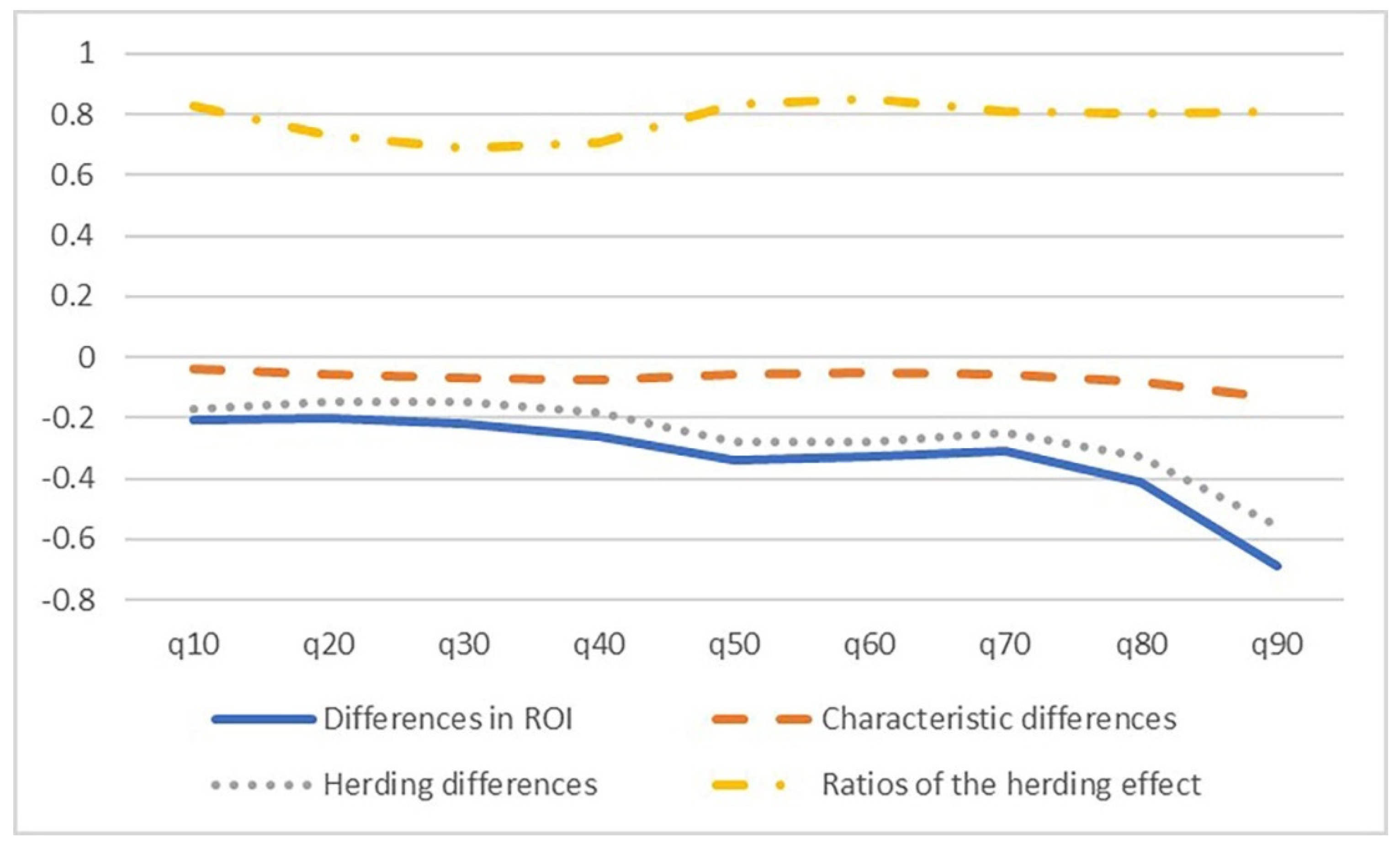
Table 8 presents the decomposition results of the difference in ROI, along with the ratios of the herding effect and the characteristic effect across quantiles. Similarly, the second column on the left represents the difference in ROI between the two groups, with and without the herding effect
, and is then decomposed into characteristic differences and herding differences. The ROI difference negatively increases in value from q10 to q90 (as shown in
Figure 4 with a solid line), indicating that the herding effect is unfavorable for investments. For the purpose of increasing profitability, professional knowledge is necessary. As shown in
Figure 4, the trend of the herding effect differences fluctuates along with the differences in ROI, indicating that the herding difference is the main factor influencing the ROI difference. In addition, the proportion of herding differences is also high (68%~85%), indicating that a simple herding behavior is not enough to cope with the complex investment environment currently; hence, the ROI worsens (dotted line in
Figure 4). To briefly conclude, only with sufficient investment literacy and skills and by avoiding herding behavior, investment return can be assured and ultimately help households avoid investment predicaments.
6. Conclusions
The major finding from employing quantile regression-based decomposition is that regardless of whether the investment return or ROI is used as dependent variable, as the quantile increases, the differences in stock investment profitability and the herding effect expand in opposite directions. Moreover, the herding effect’s high proportion in total differences provides solid evidence of it being the main reason for differences in stock investment profitability. The quantile regression decomposition reinforces our finding that differences in the herding effect are a major factor influencing investment returns. Furthermore, the empirical results presented in this study provide support for the four hypotheses proposed in
Section 2.6. First, the significant and negative association between self-reported herding behavior and both investment return and ROI confirms Hypothesis 1, indicating that households exhibiting stronger herding tendencies tend to experience poorer investment outcomes. Second, the quantile regression results reveal that the impact of herding is not uniform across the distribution of returns. The negative effect becomes more pronounced at higher quantiles, particularly beyond q75, thus supporting Hypothesis 2 and underscoring the importance of modeling return heterogeneity. Third, the interaction effects between herding behavior and various household characteristics—such as age, gender, income, and asset levels—demonstrate significant moderation effects. For example, income and gender show varying effects across quantiles in both investment and ROI models. These findings lend support to Hypothesis 3, which posits that demographic and financial characteristics condition the effect of herding. Finally, our analysis confirms Hypothesis 4, with the perceived credibility of market information moderating the negative association between herding and investment outcomes. Households that report higher trust in disclosed market information tend to suffer less from herding-induced losses or achieve better returns, suggesting that credible information can mitigate behavioral biases. The herding effect is detrimental to investment. Nevertheless, investors with adequate investment literacy and skills, along with the adoption of other rational methods, can avoid the pitfalls of herding behavior.
Regarding the total investment return as the dependent variable, the age variable shows a positive impact on investment returns after q90, indicating that older age positively influences investment effectiveness at higher quantiles. The cash holdings exhibit inconsistent effects across quantiles, suggesting that their influence on investment returns may depend heavily on underlying motivations, such as precautionary savings or market timing. Assets show significant effects on investment returns across all quantiles except for q50. Income exhibits a steep positive effect on investment effectiveness above q75. The herding effect for the head of the household shows significantly negative coefficients across all quantiles except for q25. In terms of ROI, male heads of the household experience fewer losses than female heads. The age variable shows better ROI at q50 and q90. Unlike the previous results concerning investment returns, assets do not have a significant effect on ROI. However, income demonstrates a significant positive effect on ROI. The herding effect in the stock market also shows a significantly negative correlation with ROI, consistent with the previous results on investment returns. If the head of the household believes in the information disclosed by the market, it is more likely that investment losses are reduced or that investment returns increase. By employing self-reported data regarding herding behavior, interesting and valuable outcomes were obtained with the quantile regression estimation method. In terms of financial literacy education, the government could launch comprehensive investor education programs aimed at novice investors, including free public courses and official knowledge platforms. Events such as ‘Rational Investment Month’ and ‘Anti-Speculation Week’ can heighten awareness of market sentiment risks. Establishing financial content disclosure guidelines for self-media, requiring clear information sourcing and risk disclaimers, could enhance information quality. Collaborations with social platforms to introduce content review systems or delayed posting mechanisms for speculative posts, along with regularly published ‘Hot Stock Risk Reports,’ can collectively help mitigate excessive market herding behavior
As the quantile estimation results vary significantly across distributions, it is imprudent to conclude that the observed differences in the data are solely due to this factor. However, similar results to those in the literature have been obtained. Compared with traditional methods such as the mean reversion process or the conditional distribution assumption, employing the quantile regression model provides a new perspective for relevant studies. Empirical evidence from markets such as the U.S., Hong Kong, and Japan shows increasing return dispersions, implying a weaker presence of herding behavior—consistent with the findings of Christie and Huang (
Christie & Huang, 1995). In contrast, emerging markets like South Korea and Taiwan exhibit lower-equity-return dispersions, indicating stronger herding tendencies, which aligns with our findings (
E. C. Chang et al., 2000). Furthermore, studies have identified cross-market herding effects in the U.S., UK, and Germany, where investor sentiment in one market can influence herding behavior in another, particularly among European markets (
Economou et al., 2018). In fact, the different empirical results found in this study are inconsistent with past findings, obtained by focusing only on the mean. Therefore, in future research, combining theories and experimental evidence from economics and other social sciences can enhance our understanding of how rationality and emotions interact to create herding effects in the financial sector. By collecting more independent variables, insights regarding how investors’ financial literacy, information asymmetry, and various investment portfolios influence their responses can be discovered. This behavior will reflect the response of a well-functioning market to public information. While several variables show statistically significant coefficients at specific quantiles, including risk literacy, social trust, and happiness, these results often lie near conventional significance thresholds or lack theoretical consensus. Accordingly, they should be interpreted with caution, and future research may help validate or clarify these relationships. Additionally, while some behavioral variables such as risk literacy show statistically significant effects at lower quantiles, these results remain close to the margin of significance. Hence, interpretations must be made with appropriate caution, and further empirical validation is warranted.


