1. Introduction
There are values of unknown parameters of interest in data analysis that cannot be determined even in the most favorable situation where the maximum amount of data is available, i.e., when the distribution of the population is known. This difficulty has been tackled by either introducing criteria securing that the parameter of interest is (local) identifiable or by delineating the set of observationally equivalent values of the parameter of interest; for a review of these approaches, see, e.g., (
Paulino and Pereira 1998) or (
Lewbel 2019). This note contributes to these efforts by studying the criterion for identifiability based on the minimization of the Hellinger distance, which was introduced by
Beran (
1977), and exhibiting its relationship to the criterion for local identifiability based on the non-singularity the Fisher matrix, which was introduced by
Rothenberg (
1971). The similarities and differences between these two criteria for identifiability have so far not been studied.
The main result in this note is to show that the Hellinger distance criterion can be used to verify the (local) identifiability of a parameter of interest, or lack of it, either in models or points in the parameter space where the Fisher matrix criterion does not apply. This note illustrates this result with several examples, including a parametric procurement auction model, the uniform, normal squared, and Laplace location models. These models are either
irregular because the support of the observed variables depends on the parameter of interest or the parameter space has
irregular points of the Fisher matrix. Additional examples of
irregular models and models with
irregular points of the Fisher matrix are referenced below after defining the concepts of a
regular point of the Fisher matrix and a
regular model according to conventional usage, see, e.g.,
Rothenberg (
1971).
Let
Y be a vector-valued random variable in
with probability function
. Let the available data be a sample
of independent and identically distributed replications of
Y. Consider a family
of probability density functions
defined with respect to a common dominating measure
, which will allow us to dispense with the need to distinguish between continuous and discrete random variables.
1 Let
denote a subset of densities in
indexed by
, where the parameter space
is a subset of
, with
K a positive integer. Let
denote an element of
.
Definition 1 (Identifiability). A parameter point in Θ is said to be identifiable if there is no other θ in Θ such that for μ-a.s y.
Definition 2 (Local Identifiability). A parameter point in Θ is said to be locally identifiable if there exists an open neighborhood of containing no other θ such that Yes, it has been for μ-a.s y.
Definition 3 (Regular Points)
. The Fisher matrix is the variance-covariance of the score ,The point is said to be a regular point of the Fisher matrix if there exists an open neighborhood of in which has constant rank.
The (local) identifiability of regular points of the Fisher matrix in parametric models has been extensively studied, see, e.g.,
Rothenberg (
1971). In contrast, the identifiability of irregular points has been less studied and the literature is rather unclear about what may happen about (local) identifiability of irregular points of the Fisher matrix. The study of irregular points is worthy of consideration because, first, there are several models of interest with this type of point in the parameter space (see the list below), and second, because irregular points may either correspond to:
points in the parameter space that are not locally identifiable and for which a consistent estimator cannot not exist, e.g., the measurement error model studied by
Reiersol (
1950), or a consistent estimator can only exist after a normalization; or
points in the parameter space that are locally identifiable and for which a
-consistent estimator cannot exist (and some algorithms, e.g., Newton–Raphson method based on the Fisher matrix, will face difficulties in converging) or a
-consistent estimator can only exist after a reparametrization of the model, see, e.g., the bivariate probit model in
Han and McCloskey (
2019).
Hinkley (
1973) noted that an irregular point of the Fisher matrix arises in the normal unsigned location model when the location parameter is zero.
Sargan (
1983) constructed simultaneous equation models with irregular points of the Fisher matrix.
Lee and Chesher (
1986) showed that the normal regression model with non-ignorable non-response has irregular points of the Fisher matrix in the vicinity of ignorable non-response.
Li et al. (
2009) noted that finite-mixture density models have irregular points of the Fisher matrix in the vicinity of homogeneity.
Hallin and Ley (
2012) showed that skew-symmetric density models have irregular points of the Fisher matrix in the vicinity of symmetry. We use below the normal squared location model (see Example 3) to illustrate in a transparent way the notion of an irregular point of the Fisher matrix.
The next Section shows that the criterion for local identifiability based on minimizing the Hellinger distance, unlike the criterion based on the non-singularity of the Fisher matrix, does apply to both regular and irregular points of the Fisher matrix and to
regular and
irregular models, to be defined below in
Section 3.
Section 3 shows that, for regular points of the Fisher matrix in the class of
regular models studied by
Rothenberg (
1971), the criterion based on the Fisher matrix is a particular case of the criterion based on minimizing the Hellinger distance (but not for
irregular models or irregular points of the Fisher matrix).
Section 4 relates the minimum Hellinger distance criterion with the criterion based on the reversed Kullback–Liebler criterion, introduced by
Bowden (
1973), by showing that both are particular cases of the criterion for identifiability based on the minimization of a
-divergence.
2. The Minimum Hellinger Distance Criterion
Identifying
is the problem of distinguishing
from the other members of
. It is then convenient to begin by introducing a notion of how densities differ from each other. The squared Hellinger distance for the pair of densities
in
is the square of the
-norm of the difference between the squared-root of the densities:
The squared Hellinger distance has the following well-known properties (see, e.g.,
Pardo 2005, p. 51), which are going to be used later.
Lemma 1. ρ can take values from 0 to 1, which are independent of the choice of the dominating measure μ, and if and only if for μ-a.s y.
(All the proofs are in
Appendix A) Alternative notions of divergence between densities, other than the squared Hellinger distance, are studied in the
Section 4. Since
is equal to zero if and only if
and
are equal, one has the following characterization of identifiability.
Lemma 2. The parameter is identifiable in the model if and only if, for all such that , .
Moreover, since is non-negative and reaches a minimum at , one obtains the following criterion for identifiability based on minimizing the squared Hellinger distance.
Proposition 1. The parameter is identifiable in the model if and only if This criterion applies to models where:
the support of Y depends on the parameter of interest (see Examples 1 and 2 below);
is not a regular point of the Fisher matrix (see Example 3 below);
some elements of the Fisher matrix are not defined (see Example 5 below);
is not continuous (see Example 6 below);
Θ
is infinite-dimensional, as in semiparametric models (which are out of the scope of this note).2
The following examples illustrate the use of Proposition 1 and the definitions introduced so far. They are also going to illustrate, in the next section, the regularity conditions employed by
Rothenberg (
1971) to obtain a criterion for local identifiability based on the Fisher matrix. In these examples,
denotes the Lebesgue measure. The
Supplementary Materials presents step-by-step calculations of the squared Hellinger distance in Examples 1–5.
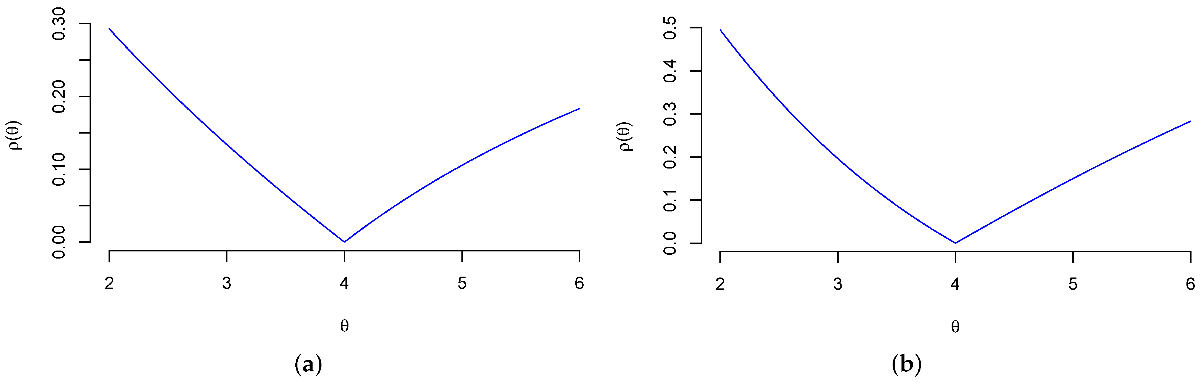
Example 1 (Uniform Location Model)
. Set and . Consider the uniform location modelThe Hellinger distance is Since the unique solution to is , see Figure 1a, one has . The Fisher matrix is , which is a singular matrix.
Example 2 (First-Price Auction Model)
. Consider the first-price procurement auction model with m bidders introduced in (Paarsch 1992, Section 4.2.2). For bidders with independent private valuations, following an exponential distribution with parameter θ (Paarsch 1992, Display 4.18) shows that the density of the wining bid in the i-th auction isSet and . The Hellinger distance in this case is For (resp. ), one has (), see Figure 1b. Hence, by continuity of , . The Fisher matrix is , which is a singular matrix. Example 3 (Normal Squared Location Model)
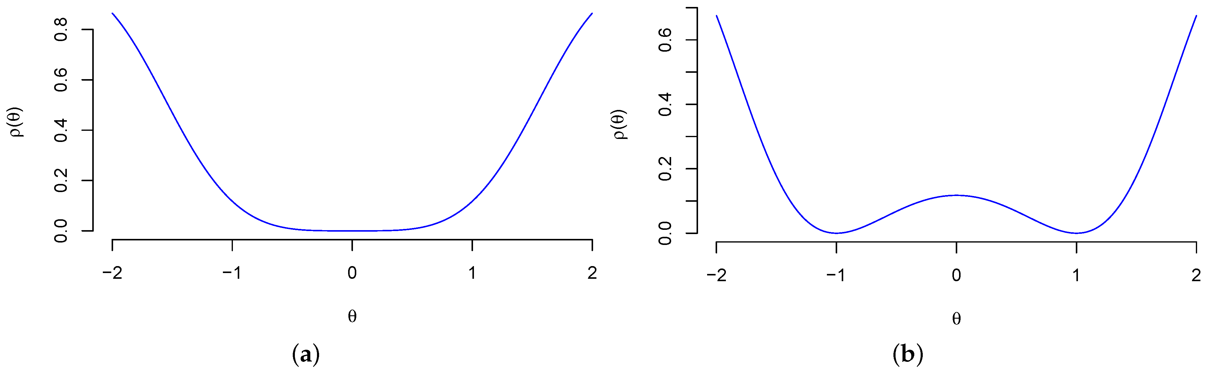
. Set and . Consider the normal squared location modelThis model would arise, for example, if Y is the difference between a matched pair of random variables whose control and treatment labels are not observed. The Hellinger distance is The parameter point is identifiable because is a strictly convex function, see Figure 2a. The parameter points are not identifiable because , see Figure 2b. The Fisher matrix is , which implies that is a singular matrix and is an irregular point of the Fisher matrix. Example 4 (Demand-and-Supply Model)
. Let denote the observed price and quantity of a good transacted in a market at a given period of time. Linear approximations to the demand and supply functions arewhere are unknown parameters and is an unobserved random vector. Assume that U and V are independent and jointly normal distributed with mean zero and unknown variance and , respectively. Set . The density of the observed variables is thenwhere is the determinant of the matrix in the parenthesis andThe squared Hellinger distance is To show that is not identifiable, by Proposition 1, it suffices to verify that is not a singleton. We elaborate on this point in the Supplementary Material. Example 5 (Laplace Location Model)
. Set , . Consider the Laplace location modelThe squared Hellinger distance is For any (), one has (). By continuity, has then a unique minimizer at , and, by Proposition 1, is identifiable. The Fisher matrix is , which is a non-singular matrix.
Example 6 (Exponential Mixture)
. Set , and . Consider the finite mixture of exponential modelConsider and . Since , one has and . Since , it follows from Proposition 1 that is not identifiable.
The previous examples also illustrate the difference between identifiable and local identifiable points in the parameter space.
Example 7 (Normal Squared Location Model, Continued)
. In this example, any is locally identifiable—even the irregular point to the Fisher matrix—and only is identifiable, see Figure 2. We also have the following criterion for local identifiability based on minimizing the squared Hellinger distance.
Proposition 2. The parameter is locally identifiable in the model if and only if there exists an open set such that This criterion, unlike the criterion based on the Fisher matrix by Rothenberg (1971) and re-stated below as Lemma 3 for the sake of completeness, applies to the case when: the support of Y depends on the parameter of interest;
is not a regular point of the Fisher matrix;
some elements of the Fisher matrix are not defined;
is not continuous;
Θ is infinite-dimensional.
Proposition 2 reduces local identifiability to a unique solution of a well-defined minimization problem. One general criterion, and, as argued, e.g., (
Rockafellar and Wets 1998), virtually the only available one, to check in advance for the uniqueness of a minimizer of an optimization problem is the strict convexity of the objective function. The application of this general criterion to the characterization of local identifiability in Proposition 2 yields the following result:
Proposition 3. If is a locally strictly convex function around (i.e., if there is an open convex set such that is a strictly convex function), then is locally identifiable.
Proposition 3 leads to the observation that local identifiability can be seen to be related to the local convexity of the Hellinger distance. As with our earlier propositions, it holds when the support of Y depends on the parameter of interest, is not a regular point of the Fisher matrix, some elements of the Fisher matrix are not defined or is not continuous.
3. The Fisher Matrix Criterion
Rothenberg (
1971) gives a criterion for local identifiability in terms of the non-singularity of the Fisher matrix. Additional insight about the relevance—and limitations—of the Fisher matrix criterion for local identifiability may then be gained by relating it to the criterion based on minimizing the Hellinger distance. To study this relationship, we now focus on the
regular models studied by
Rothenberg (
1971).
Assumption 1 (R (Regular Models)). is such that:
(A1) Θ is an open set in .
(A2) and for all .
(A3) is the same for all .
(A4) For all θ in a convex set containing Θ and for all , the functions and are continuously differentiable.
(A5) The elements of the matrix are finite and are continuous functions of θ everywhere in Θ.
We now replicate the characterization of local identifiability by
Rothenberg (
1971) Theorem 1 based on the non-singularity of the Fisher matrix.
Lemma 3. Let the regularity conditions in Assumption R hold. Let be a regular point of the Fisher matrix . Then, is locally identifiable if and only if is non-singular.
This characterization of local identifiability only applies to the regular models defined by Assumption R and to the regular points of the Fisher matrix, which may be a subset of the parameter space (see Example 3). These conditions do not have themselves any direct statistical or economic interpretation: their role is just to permit a characterization of local identifiability.
3 We have already referenced in the introduction a list of models with irregular points of the Fisher matrix, for which the characterization in Lemma 3 does not apply. We now use Examples 1–5 to illustrate the notions of regular and irregular models and their implications for the analysis of identifiability. The richness of the possibilities that follow is a recall of the care needed in using the Fisher matrix criterion for showing local identifiability (or lack of it). It also highlights the convenience of the identifiability criterion based on minimizing the Hellinger distance as a unifying approach to study the identifiability of regular or irregular points of the Fisher matrix in either regular or irregular models. Specifically:
The uniform location model in Example 1 and the first-price auction model in Example 2 have, respectively, and , which means that these models violate the regularity condition . We have seen that is identifiable in Examples 1 and 2, which implies that is not necessary for identifiability. These models also have a singular Fisher matrix, which implies that, in irregular models violating , the non-singularity of the Fisher matrix is not a necessary condition for (local) identifiability.
One can verify that the normal squared location model in Example 3 and the normal supply-and-demand model in Example 4 both satisfy the regularity conditions in Assumption R. We have seen that in Example 3 the parameter of interest is locally identifiable while in Example 4 it is not, which means that the regularity conditions in Assumption R are not sufficient or necessary for (local) identifiability, they are just convenient. In Example 3, moreover, is not a regular point of the Fisher matrix and is locally identifiable, which implies that, for irregular points of the Fisher matrix, the non-singularity of the Fisher matrix is not a necessary condition for (local) identifiability.
In Example 5, the function is not differentiable when , which means that the Laplace location model is an irregular model because it violates .
To illustrate a failure of and , consider the finite mixture of exponential model in Example 6 with , and . In this case, , which is not finite.
We also have the following result linking the Hellinger distance to the Fisher matrix, which we are going to use to show that, in regular models with irregular points to the Fisher matrix, the non-singularity of the Fisher matrix is only a sufficient condition for local identifiability.
Lemma 4. Let the regularity conditions in Assumption R hold and assume that is continuously differentiable μ-a.e. Then, the Hellinger distance and the Fisher matrix are related by Though this result is known, see, e.g., (
Borovkov 1998), its implications for local identifiability have so far not been drawn.
Since the Fisher matrix is a variance-covariance matrix, one has that
is, under
, a real symmetric semi-definite positive matrix for every
, and then the following result follows from Lemma 4 and the characterization of a convex function in terms of its Hessian, see, e.g., (
Rockafellar and Wets 1998, Theorem 2.14).
Proposition 4. Let the regularity conditions in Assumption R hold and assume that is continuously differentiable μ-a.e. Then, is a locally convex function around . Furthermore, if is non-singular, then is a locally strict convex function around and is locally identifiable.
Two remarks are in order. First, notice that, unlike Lemma 3, the result in Proposition 4 also applies when is not a regular point of the Fisher matrix and the non-singularity of the Fisher matrix becomes only sufficient for local identifiability. Second, if is singular, the function is still locally convex (because is positive semi-definite) and is a convex, but not necessarily bounded, set, which is a result that can be used to delineate the set of observational equivalent values of . This note does not pursue this interesting direction.
Table 1 summarizes the information in this note about the necessity and sufficiency of the non-singularity of the Fisher matrix for local identifiability.
We conclude this section by mentioning that, in response to the misbehavior of the Fisher matrix when informing about the difficulty to estimate parameters of interest in parametric models, alternative notions of information, other than the Fisher matrix, have been proposed in the literature (see, e.g.,
Donoho and Liu 1987). Without further elaboration, these alternative notions of information are not directly applicable to construct new criteria of identifiability. In particular, the geometric information based on the modulus of continuity of
with respect to the Hellinger distance, introduced by
Donoho and Liu (
1987) to geometrize convergence rates, cannot be used to construct a criterion for local identifiability because this modulus of continuity, in its current format, is not defined for parameters that are not locally identifiable.
4 4. The Kullback–Liebler Divergence and Other Divergences
Some of the examples where we have had success in using the Hellinger distance to analyze identifiability share the same structure: the Hellinger distance is a locally convex function, see
Figure 2, and so the results from convex optimization become available. If the Hellinger distance proves to be difficult to analyze, one can set out a criterion for identifiability based on another divergence function, such as the reversed Kullback–Liebler divergence (see, e.g.,
Bowden 1973)
One can unify the identification criteria based on the Hellinger distance and the reversed Kullback–Liebler divergence by using the family of
-divergences defined as
where
is the likelihood ratio and
is a proper closed convex function with
and such that
is strictly convex on a neighborhood of
. The squared Hellinger distance corresponds to the member of this family with
, whereas the reversed Kullback–Liebler divergence corresponds to
. The following result is an immediate consequence of the property that
is non-negative and it is equal to zero if and only if
(see, e.g.,
Pardo 2005, Proposition 1.1)).
Proposition 5. The parameter is locally identifiable in the model if and only if there exists an open set such that This result, which is a generalization of Proposition 2, shows that the choice of a
-divergence for analyzing the identifiability of a parameter of interest only hinges on the difficulty to characterize the set
for a given
-divergence. The choice of the Hellinger distance over the reversed Kullback–Liebler divergence is, however, not inconsequential when choosing
-divergence to construct an estimator for the parameter of interest. The use of the Hellinger distance may lead to an estimator that is more robust than the maximum likelihood estimator and equally efficient, see, e.g.,
Beran (
1977) and
Jimenez and Shao (
2002).
5We conclude this section with the following result showing that, for the regular models analyzed by
Rothenberg (
1971), the Hellinger distance and the reversed Kullback–Liebler divergence are both locally convex around a minimizer.
Lemma 5. Let the regularity conditions in Assumption R hold and assume that is continuously differentiable μ-a.e. Let us assume, furthermore, that, in a neighborhood of , and are twice differentiable in θ, with derivatives continuous in . Then, the Hellinger distance and the Kullback–Liebler divergence are related by


