Optimizing Energy Consumption in Public Institutions Using AI-Based Load Shifting and Renewable Integration

Abstract

This paper details the development and implementation of an intelligent energy efficiency system for an electrical grid that incorporates renewable energy sources, specifically photovoltaic systems. The system is applied in a small locality of approximately 8000 inhabitants and aims to optimize energy consumption in public institutions by scheduling electrical appliances during periods of surplus PV energy production. The proposed solution employs a hybrid neuro-fuzzy approach combined with scheduling techniques to intelligently shift loads and maximize the use of locally generated green energy. This enables appliances, particularly schedulable and schedulable non-interruptible ones, to operate during peak PV production hours, thereby minimizing reliance on the national grid and improving overall energy efficiency. This directly reduces the cost of electricity consumption from the national grid. Furthermore, a comprehensive power quality analysis covering variables including harmonic distortion and voltage stability is proposed. The results indicate that while photovoltaic systems, being switching devices, can introduce some harmonic distortion, particularly during peak inverter operation or transient operating regimes, and flicker can exceed standard limits during certain periods, the overall voltage quality is maintained if proper inverter controls and grid parameters are adhered to. The system also demonstrates potential for scalability and integration with energy storage systems for enhanced future performance.

1. Introduction

The transition to renewable energy sources (RESs) is a key component in achieving sustainable development, particularly for small localities with up to 10,000 inhabitants. Photovoltaic (PV) systems offer a viable alternative to traditional energy sources, providing a clean and decentralized means of electricity generation. However, the integration of RESs into the energy grid presents challenges, particularly in balancing generation and consumption. Advanced artificial intelligence (AI) techniques, such as neuro-fuzzy systems, have emerged as effective solutions for optimizing energy management in smart grids [1,2].

The deployment of renewable energy sources in small communities offers numerous benefits, including reduced greenhouse gas emissions, enhanced energy independence, and improved energy security. Photovoltaic systems are particularly well-suited for localities with limited energy demands and space for installation. Residential rooftops, schools, and public buildings can host PV panels, effectively harnessing solar energy. This localized approach minimizes energy losses during transmission and maximizes resource utilization.

Smart grids enable efficient energy management by dynamically balancing supply and demand. The integration of PV systems within smart grids is crucial for optimizing energy usage in localities with limited energy infrastructure. Key features of smart grids include demand response strategies, predictive analytics, and AI-driven optimization mechanisms [3].

A major challenge in small localities is the variability of solar energy production due to weather conditions. To address this, predictive models based on historical data and real-time meteorological inputs are used to optimize scheduling and energy storage strategies [4].

Balancing energy generation and consumption is essential to avoid grid instability. Traditional control strategies struggle to accommodate fluctuating PV outputs, leading to energy wastage or deficits. AI-driven models, such as neural networks and fuzzy logic controllers, offer robust solutions for demand-side management [5].

Neuro-fuzzy systems combine the learning capabilities of artificial neural networks (ANNs) with the interpretability of fuzzy logic, making them suitable for complex energy management tasks. These systems can process large datasets to generate optimal energy usage patterns, ensuring stability in small localities [6].

Efficient scheduling of energy consumption is vital for maximizing the benefits of PV systems. AI-based scheduling techniques have demonstrated superior performance compared to traditional methods in optimizing load distribution and minimizing energy waste [7].

Key scheduling techniques include the following: (a) rule-based scheduling: utilizes predefined rules to manage energy distribution based on priority loads; (b) optimization algorithms: genetic algorithms (GA), particle swarm optimization (PSO), and other metaheuristic methods are used to fine-tune energy allocation [8]; (c) machine learning approaches: reinforcement learning (RL) and deep learning models predict optimal load distribution patterns based on historical and real-time data [9].

Several studies have demonstrated the effectiveness of AI-based approaches in optimizing energy use in small localities. A case study in a European village successfully integrated a neuro-fuzzy system with a local PV microgrid, achieving a 20% reduction in energy waste and improved load balancing [10].

Similarly, an experimental deployment in a rural community in Asia utilized ANN-based predictive models to schedule energy consumption dynamically, leading to increased grid resilience and cost savings [11].

The application of AI, particularly neuro-fuzzy systems, holds significant potential for enhancing the efficiency of PV energy usage in small localities. Future research should focus on improving real-time adaptability, integrating decentralized storage solutions, and developing scalable models applicable to various geographic and climatic conditions.

Recent research highlights the potential of AI systems in managing distributed energy resources, with significant reductions in operational costs and improved energy utilization being reported. For example, dynamic scheduling based on AI models has led to up to a 30% reduction in peak energy consumption in case studies involving rural administrative buildings [12,13].

New approaches, such as deep reinforcement learning, edge-based load controllers, and hybrid cloud-neuro platforms, further enhance real-time decision-making in smart grid operations [14,15]. These strategies allow improved flexibility and adaptability in response to sudden changes in energy availability or demand patterns [16,17].

The concept of explainability in AI-based energy systems has gained increased attention, ensuring system decisions are interpretable and compliant with regulatory requirements [18,19].

In this context of smart grids, this paper aims to cover a key research challenge in the field, such as the development of a knowledge-based system, based on neuro-fuzzy and scheduling techniques, able to ensure optimal use of energy from RESs. Within this hybrid approach, the proposed explainable system will consider the complex interrelation between power generated from RESs in a smart grid and load producers and consumers of energy from RESs for public entity behaviours. In this paper, the smart grid is represented by a low-voltage grid in a locality with approximately 8000 inhabitants, featuring a power system based on photovoltaic panels to supply the consumption systems within the local administrative unit (public entities).

The structure of this paper is as follows: Section 2 introduces the energy management framework, including load classification and grid architecture. Section 3 presents the simulation environment and results. Section 4 details the load scheduling algorithm and neuro-fuzzy control system. Section 5 discusses the experimental validation and power quality analysis. Conclusions and future directions are presented in Section 6.

2. Energy Management Framework

2.1. Public Entity Appliance Consumption

Public entities, including local government institutions, schools, healthcare centres, and public utilities, represent significant nodes of energy consumption within a community. Efficient energy management in these entities is critical to reducing operational costs, enhancing sustainability, and ensuring continuous service delivery. In localities with approximately 10,000 inhabitants, such entities serve as pillars of public infrastructure, with daily operations reliant on a wide range of electrical equipment [20,21].

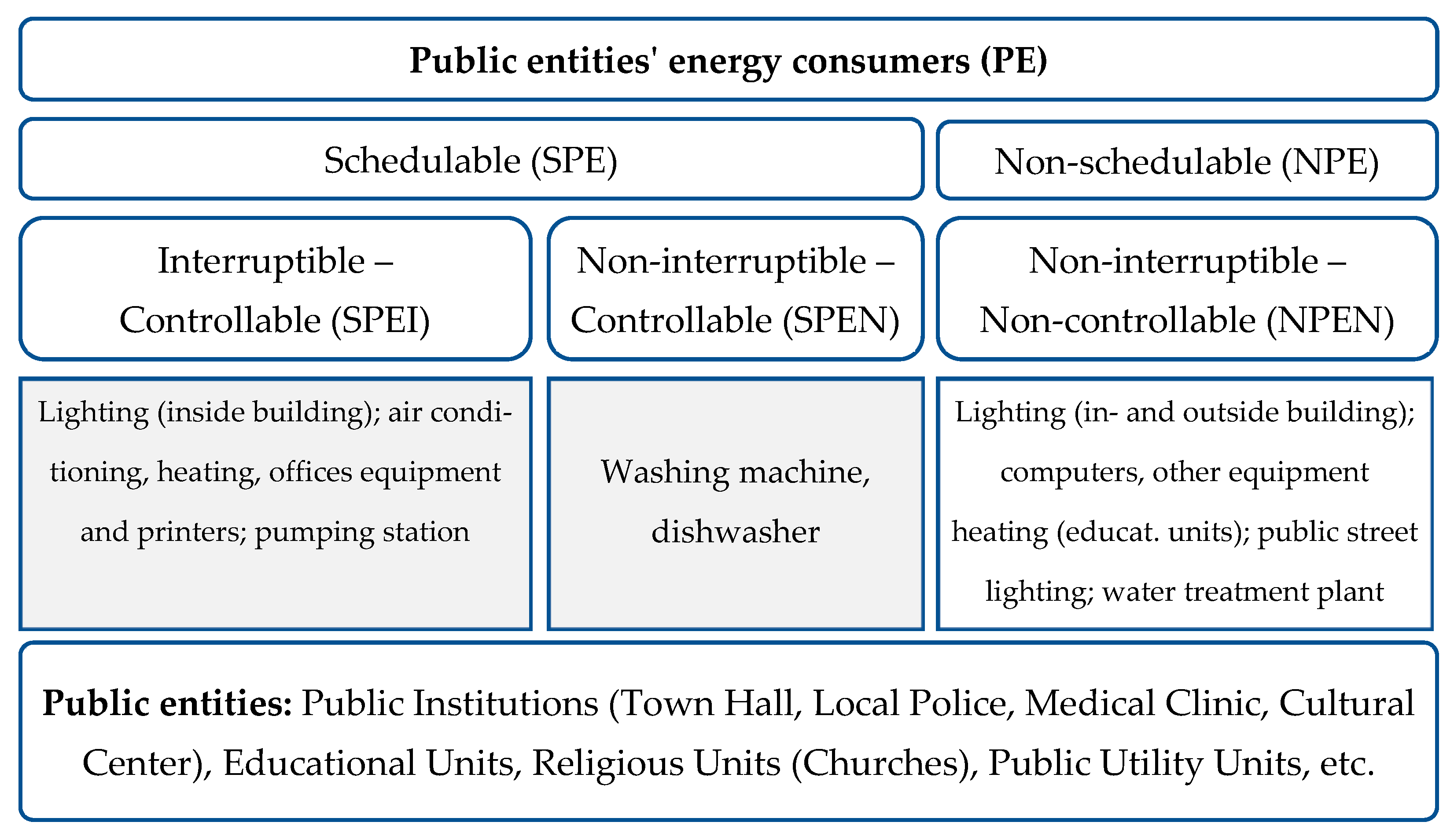
To enable targeted energy optimization, the electrical appliances used by public institutions are classified based on their controllability and operational flexibility. This classification leads to two major categories: schedulable (SPE) and non-schedulable (NPE) loads. Further subdivisions include interruptible and non-interruptible loads, as depicted in Figure 1.

Schedulable Public Entity (SPE) Appliances: These appliances can be managed and scheduled based on energy availability. Examples include interior and exterior lighting, air conditioning units, dishwashers, washing machines, and water pumping systems. These devices can be scheduled to operate during periods of PV energy surplus, enabling peak-shaving strategies and improving overall efficiency [22,23].

Non-Schedulable Public Entity (NPE) Appliances: These are essential systems that must operate on fixed schedules or continuously, such as public street lighting, medical equipment, and water treatment infrastructure. Although not directly schedulable, their performance and energy use can be optimized via technical upgrades and load forecasting [24].

The classification used in this study distinguishes loads by both control potential and interruptability: SPEI (Schedulable, Interruptible), SPEN (Schedulable, Non-Interruptible), and NPEN (Non-Schedulable, Non-Controllable).

Table 1. The public entity appliances considered.

Appliance	Type	Nr. of Appliances	Power (W)	Total Power (kW)	Operation Duration per Day	Total Energy per Day (kWh)
Lighting (in building)	SPEI	aprox. 150	18	2.7	8 h	21.6
	NPEN	aprox. 100	18	1.8	9 h	16.2
Lighting (out building)	SPEI	aprox. 48	100	4.8	8 h	64
	NPEN	aprox. 32	100	3.2	9 h	28.8
Air conditioning	SPEI	20	1.000	20	6 h	120
Pumping station	SPEI	1	15.000	15	8 h	120
Dishwasher	SPEN	15	1.400	1.4	1 h	21
Washing machine	SPEN	10	1.500	1.5	2 h	30
Computers and other equipment	SPEN/NPEN					50 ÷ 60
Total energy per day for SPEI						325.6 kWh/day
Total energy per day for SPEN						51 kWh/day
Total energy per year for SPEI						118.8 MWh/year
Total energy per year for SPEN						18.6 MWh/year

summarizes the primary appliances used by the public entities in the study area, including their operational parameters.

The continuity, in terms of operation time, represents the second criteria based on which SPEs can be classified as being interruptible (controllable) and non-interruptible or hold-time appliances (fixed).

The total energy ($P_{total}$), consumed at each time slot t by fixed appliances ($P_{SPEN})$, controllable appliances ($P_{SPEI}$), and non-schedulable ($P_{NPE}$), can be calculated using Equation (1):

$$P_{total}\left(t\right)=P_{SPEN}\left(t\right)+P_{SPEI}\left(t\right)+P_{NPE}\left(t\right)$$

(1)

Our research study considered the appliances mentioned in Table 1, the washing machine and the dishwasher, because of their ability to be shifted fully, or to be on certain operation cycles, for a run at later intervals. Table 1 presents the home appliances that were considered in our approach and their specific characteristics, including the load type, power consumed (W), and total energy per day (kWh). These consumption profiles form the basis for intelligent scheduling algorithms detailed in Section 4.2.

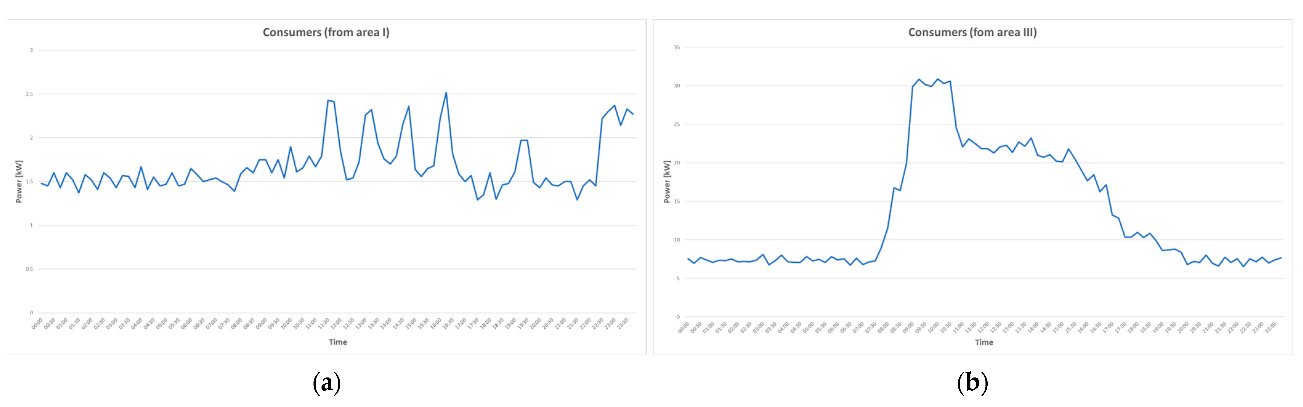
Figure 2 illustrates energy usage patterns from two representative public areas. The consumption profiles from area I (with Cultural Centre, Town Hall and Church) for lighting (in and out buildings), air conditioning, and other consumers are represented in Figure 2a (for one day—12 May 2024), and those from area III (with Educational Unit, Church and Pumping station) for lighting (in and out buildings), air conditioning, pumping station, computers, and other consumers are represented in Figure 2b (for one day—12 May 2024), which allowed us to program them with the help of shift algorithms, so that the energy produced from RESs at different times of the day could be utilized to the maximum.

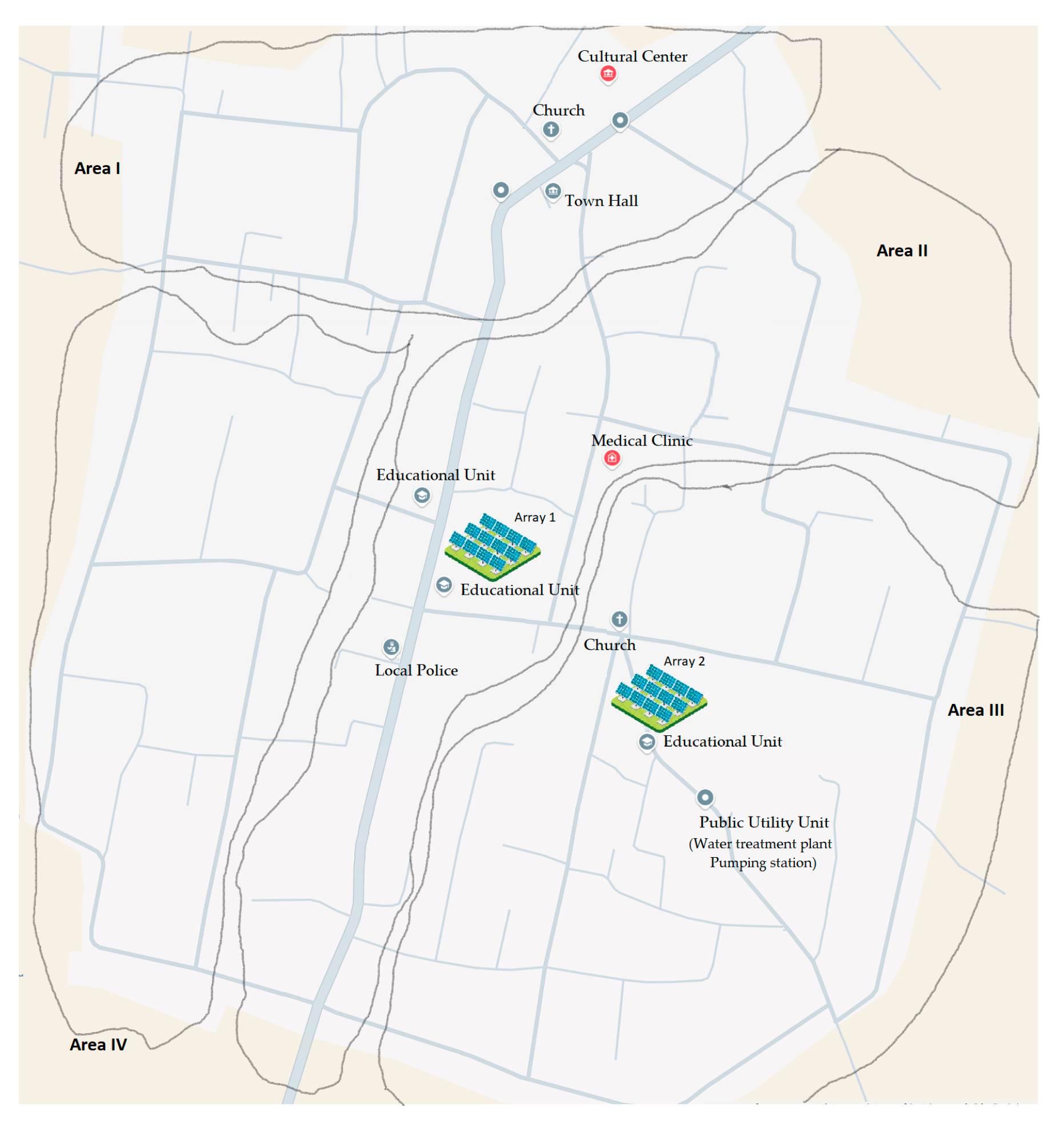
Planning energy consumption in the locality. In Figure 3, a plan of the locality is presented, highlighting the consumption points of public entities. Also, a division into four consumption areas is observed, each of these areas being connected to a voltage phase (areas I and IV to phase 1, area II to phase 2, and area III to phase 3). This plan includes the location of each institution, thus allowing for the identification of areas with high consumption and the implementation of systems for generating energy from photovoltaic sources and measures to enhance the efficiency of the produced energy utilization.

2.2. Renewable Energy Generation and Grid Architecture

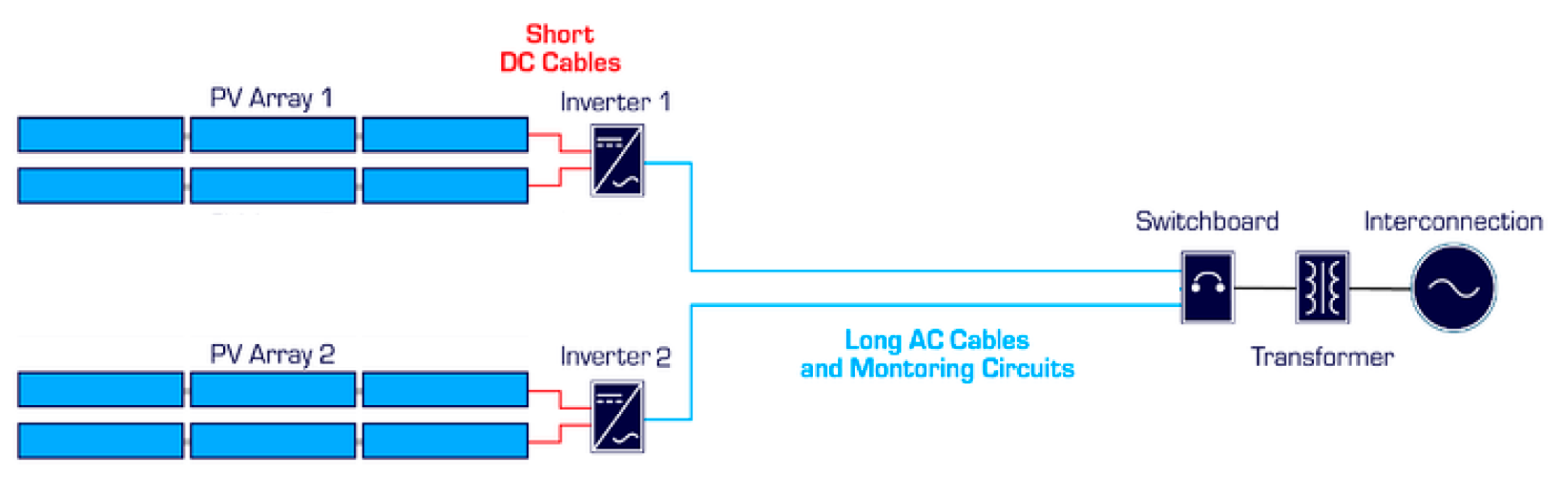
In this research, the considered smart grid was represented by public entities (territorial administrative unit) with an installed power system based on photovoltaic panels of 83.6 kWp with an estimated production per year of 97.6 MWh/year (Figure 4), smart loads, and with the possibility of operating, due to the existing connections only on grid.

Table 2. Technical characteristics of photovoltaic panels.

Model of PV panel	410 Wp, Si-monocrystalline (c-Si)
Number of panels per module	108 and 96
Nominal output power	Pnom = 410 Wp
Current at maximum power	IMPP = 13.12 A
Voltage at maximum power	VMPP = 31.25 V
Short circuit current	Isc = 13.88 A
Open circuit voltage	Voc = 37.25 V
Maximum system voltage	1000 V
Minimum efficiency	21%

lists the specifications of the 204 PV panels mounted on the ground on a fixed structure with an inclination of 35 degrees. The system that allowed for energy exchanges with the power national grid contains two inverters.

The PV array connects to the grid via SMA Sunny Boy SB2100TL inverters,(SMA Solar Technology AG, Niestetal, Germany) which feature dual-module input, flexible communication interfaces (RS485), and remote diagnostic capabilities. These inverters are selected for their high efficiency and suitability for decentralized energy systems [24].

A simplified schematic of the connection to the local distribution grid is shown in Figure 4, which includes a voltage boost converter to increase DC output to 500 V and an MPPT (Maximum Power Point Tracking) system to maintain optimal performance.

The system also includes the Sunny Data Control v5.40 software for long-term performance monitoring and configuration. Data are archived locally and used to adapt operational schedules in near real time.

In conclusion, the energy framework implemented in this study represents a scalable, intelligent infrastructure tailored to support public institutions through optimized use of renewable sources and demand-side management. The next section presents the simulation model used to validate system behaviour under realistic operating conditions.

3. Simulation of a Grid with Renewable Energy Generation

To evaluate the effectiveness of the proposed system, a detailed simulation of the local energy grid with integrated renewable generation was conducted using MATLAB R2020a/Simulink. The model replicates the configuration of the real infrastructure, including the 204 PV panels, inverters, grid connections, and key components such as MPPT controllers and load modules.

Figure 5 illustrates the overall model structure, while Figure 6 provides a detailed view of the PV module block. The model is calibrated for a nominal solar radiation of 1000 W/m² to assess maximum generation potential. The number of PV panels was selected to achieve the target output of 83.6 kW.

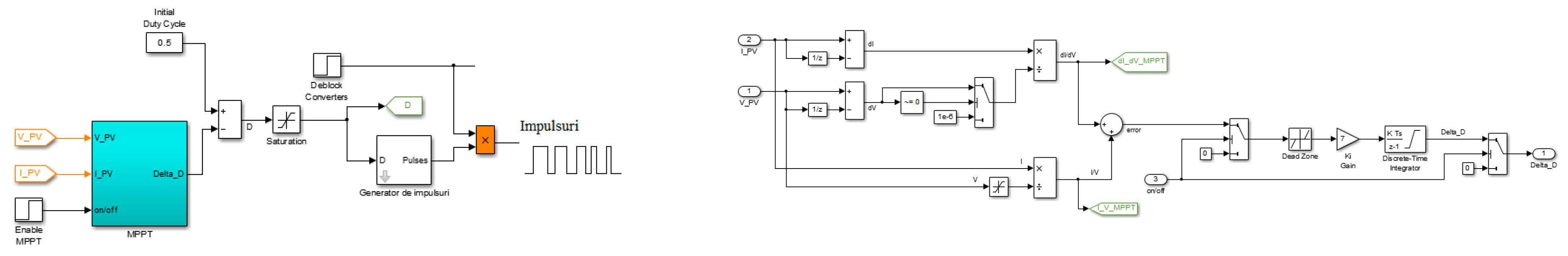
A 5 kHz boost converter was integrated into the simulation to elevate the output voltage from 216 V to 500 V. This voltage level enables maximum power transfer, governed by a proportional–integral (PI)-controlled MPPT system.

The MPPT continuously adjusts the duty cycle of the Insulated Gate Bipolar Transistors (IGBTs) to optimize energy harvesting from the PV modules. Figure 7 shows the boost converter, while Figure 7 details the MPPT implementation.

For algorithm MPPT, we used a PI controller (proportional–integral regulator) to minimize the error.

$${\displaystyle \frac{dP}{dV}}=0$$

(2)

where P is power and V is voltage. Thus,

$${\displaystyle \frac{d(V\cdot I)}{dV}}=I+{\displaystyle \frac{V\cdot dI}{dV}}=0 \to {\displaystyle \frac{dI}{dV}}=-{\displaystyle \frac{I}{V}}$$

(3)

The block IGBT is a transistor with an insulated gate and is composed of an MOS transistor and a bipolar transistor.

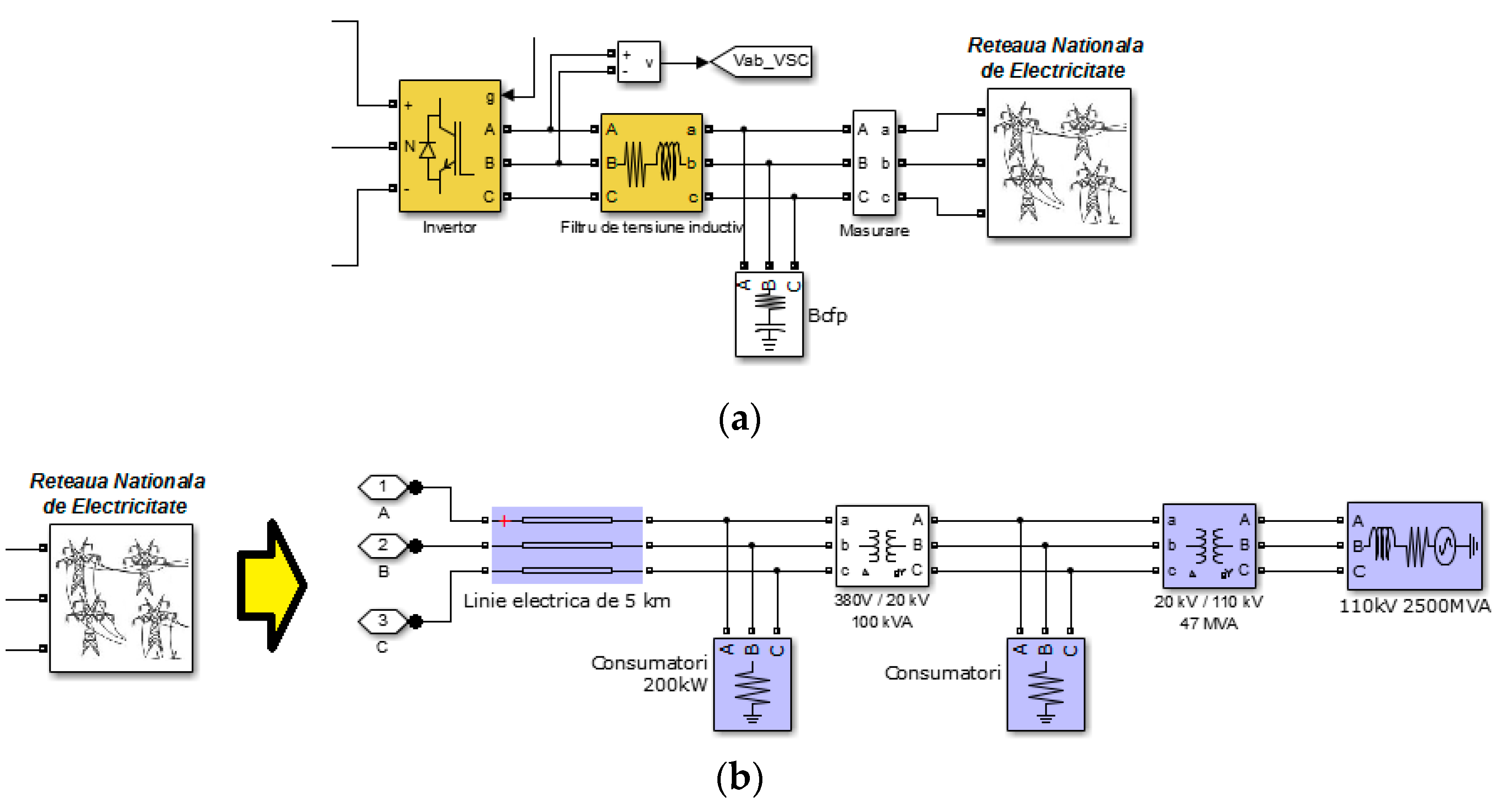
The low-voltage grid is shown in Figure 8a. It is formed of the following blocks:

• Three-phase inverter—converts DC voltage of 500 V in AC voltage of 380 V, keeping the power factor equal to 1 (cosφ = 1);
• Filtering inductive voltage harmonics—produced by the inverter;
• Power factor correction (Bcfp)—improves the power factor;
• Measuring parameters from the grid (voltage, current, and frequency);
• National energy grid with consumers (380 V).

The block of the simulation of the low voltage is shown in Figure 8b.

The block of chopper frequency generation (Figure 9), or the voltage source converter (V_SC), uses two control loops: an outer control loop that adjusts the DC voltage +/−380 V and an inner loop that adjusts the current I_d and I_q (active and reactive current component). I_d (current reference) is the output of the DC voltage external controller. I_q (current reference) is set to zero in order to maintain unity power factor.

V_d and V_q voltage outputs of the current controller are converted to three modulating signals V_{ref_abc} used by the PWM (Pulse Width Modulation) three-level pulse generator.

The simulation results, detailed in Section 5.1, demonstrate the ability of the modelled system to effectively track irradiance changes, stabilize grid voltage, and optimize inverter performance. These findings validate the proposed control strategies and form the basis for experimental deployment in the real-world scenario discussed later in the paper.

4. Load Shifting Using Scheduling Techniques

4.1. Scheduling Framework

The core objective of the proposed energy management system is to reduce the cost of electricity consumption from the national grid by intelligently scheduling the operation of electrical appliances based on the availability of renewable energy. This is formulated as a constrained scheduling problem, in which a set of tasks (appliance operations) must be optimally assigned across a set of resources (controllable appliances), considering start and end constraints.

Each task can only be initiated after a release time, and must be completed by a specific time. Each appliance has a processing time and cost function representing energy consumption. The optimization goal is to minimize the total cost while ensuring appliance-level and system-level constraints are respected.

The class of problems considered in this paper is represented by the scheduling of home appliance loads to minimize the cost paid by the producers and consumers of energy for the energy consumed from the national energy grid. This category is a scheduling one because it involves finding a least-cost schedule to process a set of orders, denoted with I, using a set of dissimilar parallel controlled or uncontrolled home appliances, denoted with M. Processing of an order i ∈ I can only begin after the release date r_i and must be completed at the latest by the due date d_i. Order i can be processed on any of the appliances. The processing cost and processing time of order i ∈ I on appliance m ∈M are Cim and Pim, respectively.

In these terms, the previously stated objectives could be formalized as follows: the main decisions involved in this scheduling problem are the assignment of orders on appliances, the sequence of orders on each appliance, and the start time for all the orders to minimize the processing cost of all the orders.

A wide variety of methods and techniques have been suggested to improve energy from RES usage through the load schedule. These methodologies can generally be grouped into five categories: mathematical optimization, heuristic and metaheuristic methods, model-based predictive control, machine learning, and game theory approaches.

We will focus in this paper on the first category of deterministic optimization-based methodologies because our problem formulation can be formalized as a linear optimization-based programming problem. In the same category of mathematical optimization-based scheduling techniques, we can identify non-linear programming problems, convex programming problems, and dynamic optimization problems. These techniques are the most popular choice for small and medium-sized scheduling problems addressed by home energy management systems. The core of the energy management problem is intelligent load shifting. In the actual European scenario to minimize energy payment, it is necessary to maximize PV energy self-consumption.

Specifically, within this study, Mixed-Integer Linear Programming (MILP) is employed as the chosen mathematical optimization approach for its suitability in handling the defined linear objective function and constraints of the energy scheduling problem.

4.2. Load Shifting Algorithm

Since the objective function and constraints in this context are strictly expressed by linear relationships, being binary programming, we have considered mixed-integer linear programming (MILP) [17] as a suitable approach.

In this context, the energy scheduling problem can be expressed (see Equation (4)) as the minimization of a cost function, given a certain number of electrical tasks N_TASKS (e.g., the appliance starts) to arrange in N_TIME time samples:

$$\underset{w,\mathit{L},\mathit{C}}{\mathit{min}}\sum _{k=1}^{N_{task}}\sum _{i=1}^{N_{time}}{w}_k\left(i\right)L_k\left(i\right)C_k\left(i\right)$$

(4)

where $w_k\left(i\right)$ express whether or not a task is running at a specific time; $C_k\left(i\right)$ is the energy cost at time i; and $L_k\left(i\right)$ is the energy consumed by the task in the time interval i.

In particular, this minimization problem is subject to the following constrains (Equation (5)–(7)) considering the total power consumed at each time and the absence of interruptions for each task:

$$\forall \overline{i}\to \sum _k{w}_k\left(\overline{i}\right).L_k(\overline{i})\le P_{max}$$

(5)

$$\forall \overline{k}\to w_{\overline{k}}\left(i\right)=1, \forall i: T^{start}<i<T^{end}$$

(6)

$$C_{\overline{k}}\left(\overline{i}\right)=\left\{\begin{array}{c}R\left(\overline{i }\right) if{\displaystyle \sum _{k\ne \overline{k}}}{w}_k\left(\overline{i}\right).L_k\left(\overline{i}\right)>P_{PV}\\ 0 if{\displaystyle \sum _{k\ne \overline{k}}}{w}_k\left(\overline{i}\right).L_k(\overline{i})\le P_{PV}\end{array}\right.$$

(7)

The shiftable tasks can set $w_k\left(i\right)$ to 1 according to a determined policy.

For each shiftable load k, we consider equation 11:

$$J\left(i\right)=\widehat{P_{PV}}\left(i\right)-\widehat{L_{TOT}}\left(i\right)$$

(8)

where: $\widehat{P_{PV}}\left(i\right)$ is the PV production forecasted at time I and $\widehat{L_{TOT}}\left(i\right)$ is the averaged consumption pattern for the considered day of the week. $\widehat{L_{TOT}}\left(i\right)$ is computed averaging the last 10 days and excluding the power consumed by the shiftable loads.

Then, we have to find the best timing to start the task minimizing the costs, as Equation (12) shows:

$$\underset{i}{min⟦J\left(j\right)-L_k\left(j\right)⟧}{C}_k\left(j\right)unde j=i,\dots ,i+T^{op}$$

(9)

where $L_k\left(j\right)$ is the power consumed by the load at relative time j; $C_k\left(j\right)$ is the energy cost; and $T^{op}$ is the total cycle time of the load.

4.3. Neuro-Fuzzy Knowledge-Based System

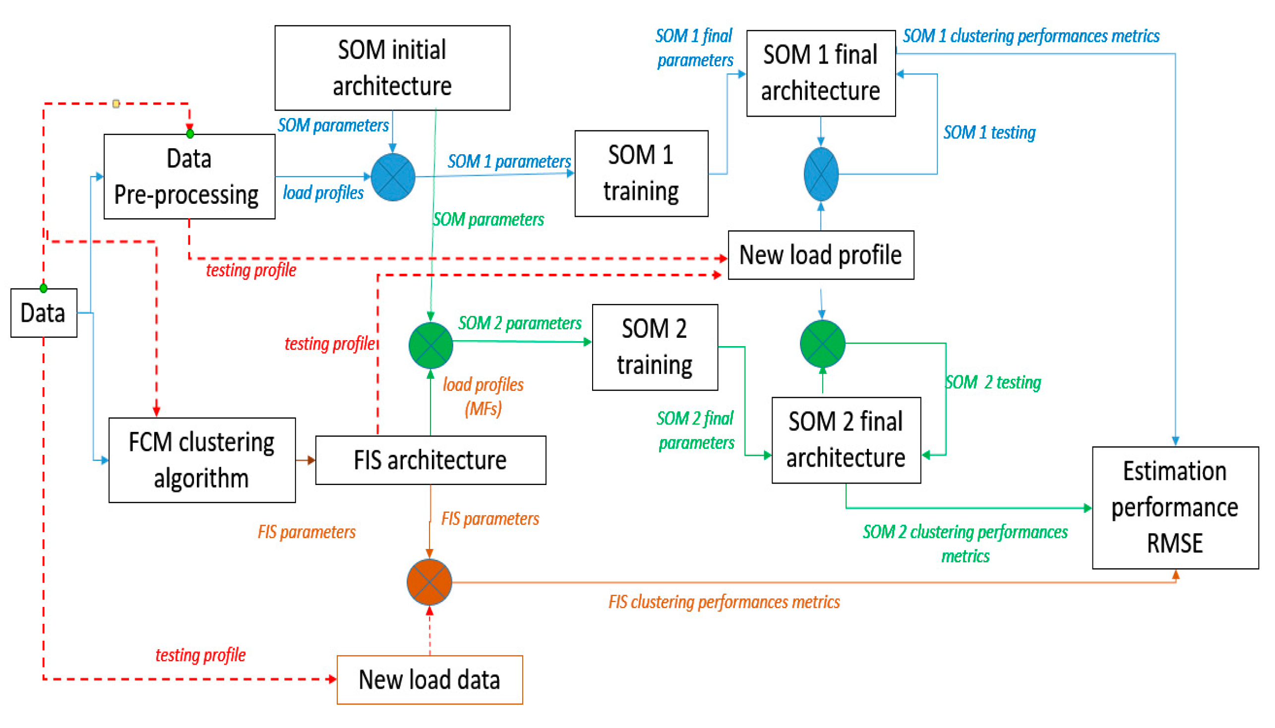
The monitored data related to load values, stored in .dat or .xls formats and correlated with the day of the week, are utilized by the Fuzzy C-Means (FCM) algorithm to extract membership functions (MFs) corresponding to a predefined number of clusters, within a maximum number of iterations. The second phase of modelling and simulation involves the automatic extraction of fuzzy rules based on the derived MFs, followed by the construction of a fuzzy rule base. These rules are expressed in a verbose format using linguistic terms. Subsequently, the root mean square error (RMSE) is calculated during the training and testing phases, in relation to the objective function. The FCM process follows an iterative loop consisting of problem initialization, Euclidean distance computation, and cluster updating steps (Figure 10a).

In contrast, the Self-Organizing Map (SOM) based on the Kohonen network begins with the configuration of its architecture, including topology, number of training epochs, input dataset, distance function, and grid representation. The network is then trained and evaluated to classify consumer load profiles. For the SOM training set, the user uploads actual consumer data from the monitored database. The training algorithm runs over several user-defined epochs, as specified in the neuro-fuzzy system interface. After training, the tool allows for evaluation and visualization of network performance metrics such as topology, neighbourhood structure, distance between nodes, sample distribution, and the positioning of SOM weights (Figure 10b).

4.4. System Testing and Visualization

First, we assessed the clustering performance of the Self-Organizing Map (SOM) by varying the input data used for training. An initial SOM architecture was defined, and for this configuration, we used the consumer load profiles described in Section 4.2 as the training dataset.

The SOM was trained using batch learning, where weights and biases are updated only after a complete pass through the entire dataset. Training concludes when the predefined maximum number of epochs is reached. This parameter was varied in order to observe and evaluate the impact on the SOM’s performance during this phase.

Upon completion of training, the SOM configuration yielding the best performance—based on topology and distance function—was designated as SOM1 (Figure 11). In our experiments, the hexagonal topology combined with the link distance function produced the most effective clustering results.

In a second scenario, we trained the SOM using profiles previously generated by the FCM clustering algorithm, as described in Section 4.1. After this training process, the resulting SOM configuration was referred to as SOM2 (Figure 11).

The proposed neuro-fuzzy tool provides the capability to evaluate and visualize the performance of the SOM network by analysing elements such as neighbour connections, inter-neuron distances, sample hits, and the positions of SOM weight vectors. During the testing phase, SOM1 and SOM2 are evaluated using a new input profile that was not included in the initial parameterization or training phase (Figure 10b).

Figure 12a illustrates the SOM layer, where neurons are shown as grey-blue patches and their direct neighbour relationships are highlighted with red lines. The SOM is organized using a two-dimensional topology, and the relationships between cluster centres can be observed in the weight distance matrix, also known as the U-matrix (Figure 12b). In this figure, blue hexagons represent the neurons, while red lines indicate the connections between neighbouring neurons.

The colour gradients in the regions where red lines appear represent the distances between neurons—darker shades correspond to greater distances, while lighter shades indicate smaller distances. A prominent dark band, indicating high inter-neuron distances, spans diagonally from the lower-right to the upper-central area.

The relative number of input vectors associated with each neuron is depicted by the size of the colour patches in Figure 12c, which visualizes the SOM layer with each neuron sized proportionally to the number of classified vectors. Figure 12d displays the input data overlaid on the SOM weight vectors. In this figure, green dots represent the input vectors, while blue-grey dots represent the SOM weight vectors. Neighbouring neurons are again connected with red lines, illustrating how the SOM classifies and structures the input space.

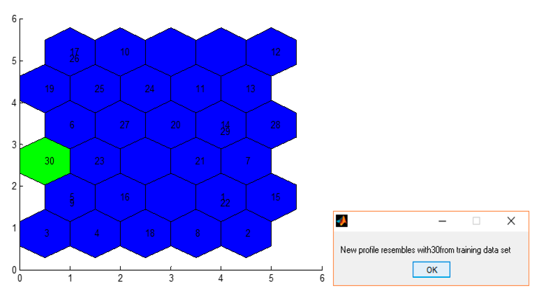
Since SOM training does not require a specified target output, unlike many other types of neural networks, its performance is evaluated using the winning node—also known as the Best Matching Unit (BMU). This BMU is identified and displayed in green in Figure 13.

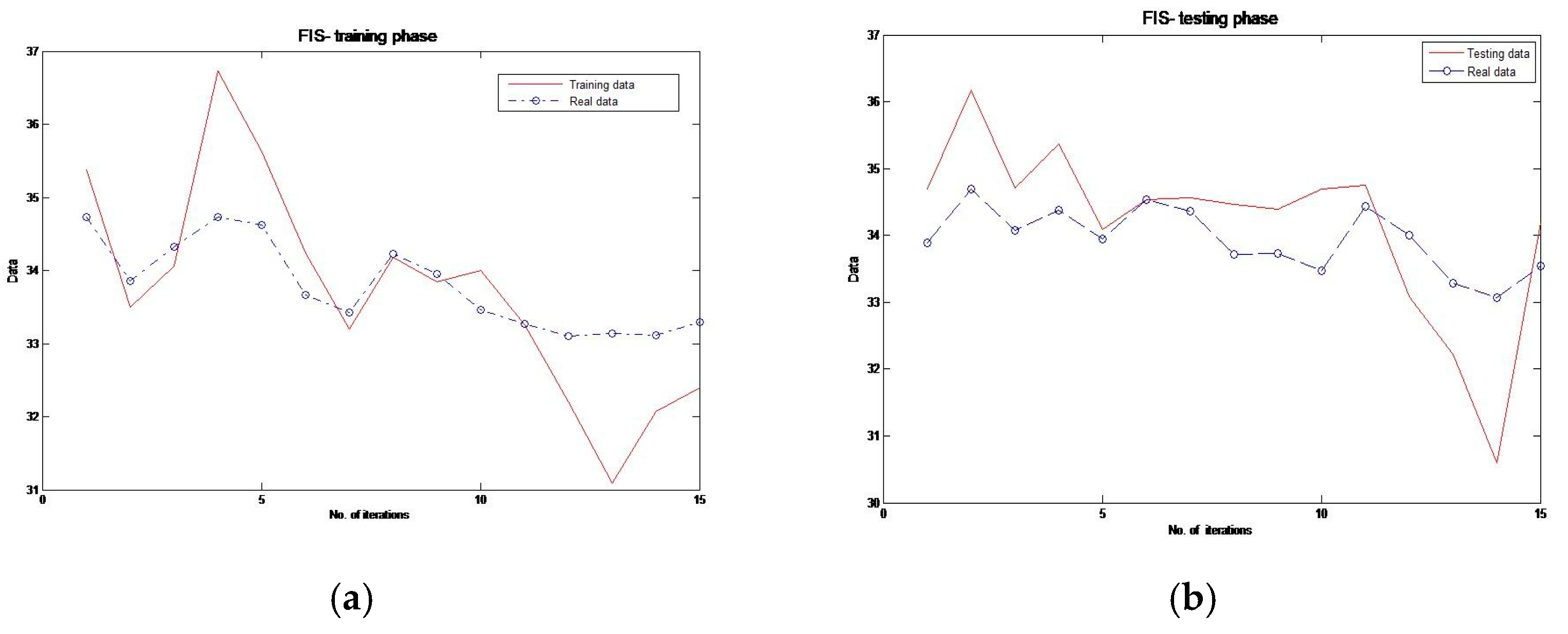
Secondly, we compared the clustering performance of SOM1, SOM2, and the Fuzzy Inference System (FIS). The data flow used in this comparison followed the same scenario as previously described. Additionally, the progress of the FIS, using the FCM clustering process as its objective function, can be visualized. With each iteration, the FCM algorithm minimizes this function to determine the optimal placement of clusters, and the corresponding values are displayed graphically. The evolution of FIS error rates during both training and testing phases is shown in Figure 14.

Our study identified the strengths and limitations of each clustering method. Specifically, both FCM and SOM perform well when the number of clusters is small, or the dataset size is limited. Increasing the number of samples from 100 to 300 generally leads to a modest improvement in error rates. For example, SOM demonstrated a slight reduction in RMSE—from 0.65 to 0.50—when more samples were introduced. In contrast, the FCM algorithm yielded a more substantial improvement, reducing RMSE from 0.71 to 0.48.

However, as the number of clusters increases, or when dealing with high-dimensional data, error rates also tend to rise. Despite this, SOM clustering remains highly effective for data visualization. Its low-dimensional grid representation offers valuable insights into the data structure by revealing spatial relationships among clusters.

4.5. Determining Optimal Load Shifting Using Scheduling Techniques

The energy-consuming appliances considered in the scenarios reported here were selected from those presented in the section dedicated to the public entity appliance consumption. The consumption profiles of SPEs from Table 1 are considered to be, in our scenarios, priority controllable consumers, meaning loads whose consumption interval can be established according to the energy produced from RESs, but for equipment from the SPEN category, once turned on, it is preferable not to be turned off. In addition, they have the ability to be shifted, fully or on certain operation cycle (see

Table 3. Washing machine power consumption during the operating cycles.

Operating Phase	Min. Power (W)	Max. Power (W)	Operation Time (min)
Movement	27.2	2100	26
Pre-heating	5	300	6.6
Heating	206.5	2200	59.7
Maintenance	11.0	200	19.9
Cooling	10.8	500	10
1st rinse	10.3	700	10.4
2nd rinse	9.9	700	10.3
3rd rinse	23.6	1170	19.8

for washing machine), for a run at later intervals.

On the other hand, the SPEI consumption profiles from Table 1 are interruptible controllable consumers because the consumption interval can be set according to the energy produced, and their operation can be interrupted.

In addition to these controllable consumers, in our case, uncontrollable consumers NPE from Table 1 were also taken into account. Two scenarios presented in Section 5.2.2 were considered: scenario 1 for 15 May 2024 and scenario 2 for 17 May 2024.

Limited historical data can impact the accuracy of the neuro-fuzzy forecasting and scheduling system, though the system demonstrates some robustness. Both Fuzzy C-Means (FCM) and Self-Organizing Map (SOM) algorithms, which rely on monitored historical load data, show improved error rates with an increased number of samples. For example, SOM’s Root Mean Square Error (RMSE) reduced from 0.65 to 0.50, and FCM’s decreased from 0.71 to 0.48, when samples were increased from 100 to 3002.

For unusual load events or highly dynamic environments, the system faces the challenge of limited real-time adaptability. While it currently adapts operational schedules in near real-time using local data archiving and monitoring, future research is directed towards enhancing this with deep reinforcement learning and edge-based load controllers to improve flexibility and adaptability to sudden changes in energy availability or demand patterns.

5. Results

5.1. Simulation Results

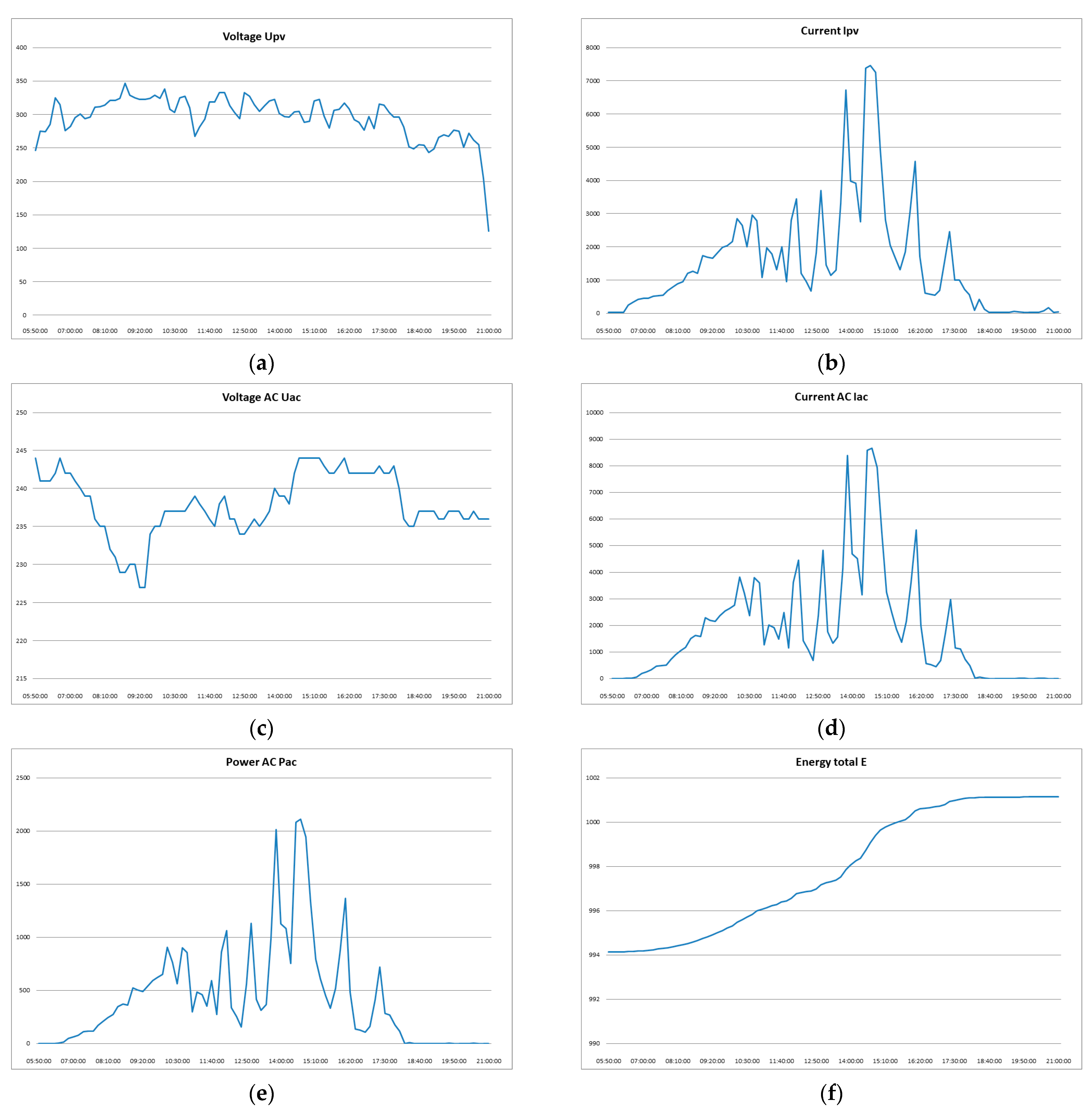
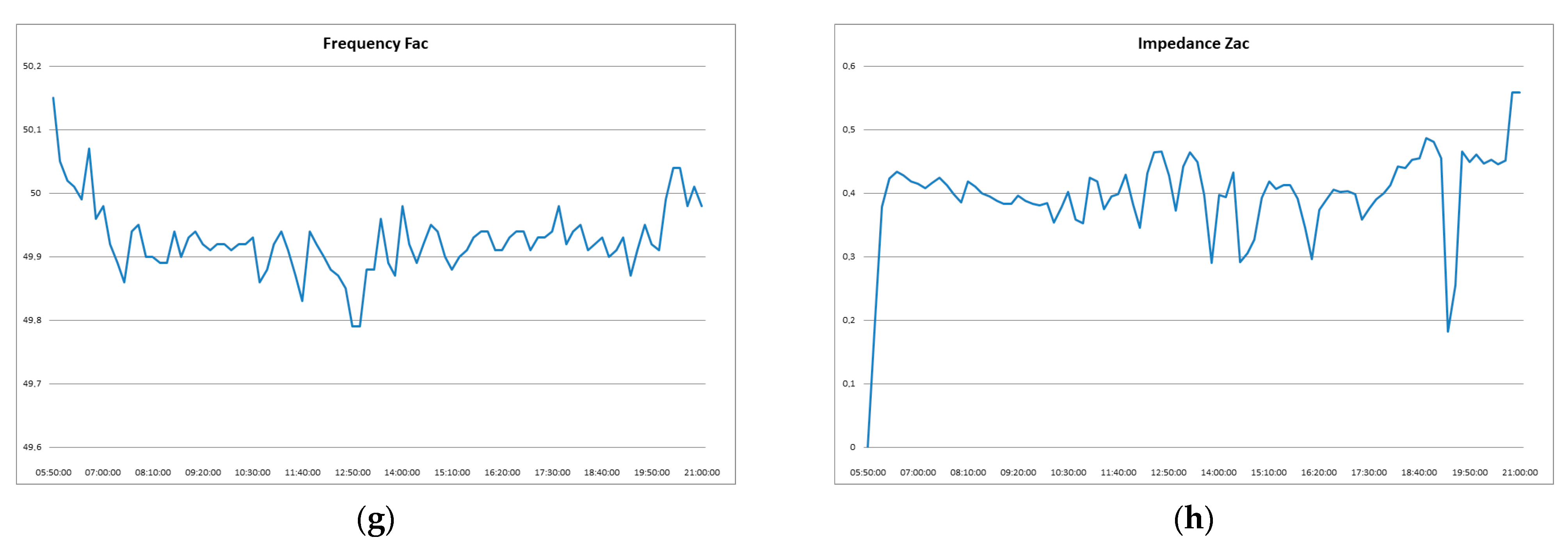
The proposed system was simulated for one day (12 May 2024) and a four-day period (12 May 2024–15 May 2024). Data were acquired at 15-min intervals to analyse the dynamics of power generation and delivery from the photovoltaic installation.

Figure 15 presents simulated parameters for the single-day test, including DC-side voltage and current from PV modules (Upv, Ipv), AC-side values (Uac, Iac), power output (Pac), cumulative energy generation, output frequency, and impedance variation.

Figure 16 extends the observation period, showing daily AC power and energy trends. These simulations validate the effective performance of the system under real irradiation profiles and highlight the inverter’s ability to maintain consistent output despite irradiance variation.

From these outputs, we conclude that the MPPT controller reliably tracks the optimal operating point. Moreover, the system exhibits resilience to transient environmental changes and maintains efficiency in PV conversion and energy delivery.

Beyond simulation, several real-world factors could negatively impact the intelligent energy efficiency system’s performance, but mitigation strategies are in place or planned. The variability of solar energy production due to weather is addressed by predictive models using historical data and real-time meteorological inputs, alongside AI-driven neuro-fuzzy systems that optimise scheduling and energy usage patterns to maintain stability.

In addition, while harmonic distortion from PV inverters is observed, power quality analyses indicate that overall power quality remains within standard limits [25,26], confirming that proper inverter controls prevent voltage quality compromises.

Grid instability from fluctuating PV outputs is mitigated by AI-driven optimisation mechanisms and demand response strategies, with the load shifting algorithm aligning energy-intensive operations with peak PV generation, reducing national grid dependency.

Although limited real-time adaptability in dynamic environments is a challenge, the system currently uses local data archiving and monitoring (Sunny Data Control software) to adapt operational schedules in near real time.

Future research aims to enhance this with deep reinforcement learning and edge-based load controllers. The applicability to diverse geographic and climatic conditions and the absence of integrated energy storage systems are recognised as areas for future research to develop more scalable models and integrate storage solutions.

5.2. Experimental Results

5.2.1. Inverter Monitoring

Data from inverters located in Area III were monitored over a one-day interval (15 May 2024) and over a one-week period (12–18 May 2024). Figure 17a,b display power output profiles, demonstrating consistency in the PV system’s operation and validating the simulation results under real-world conditions.

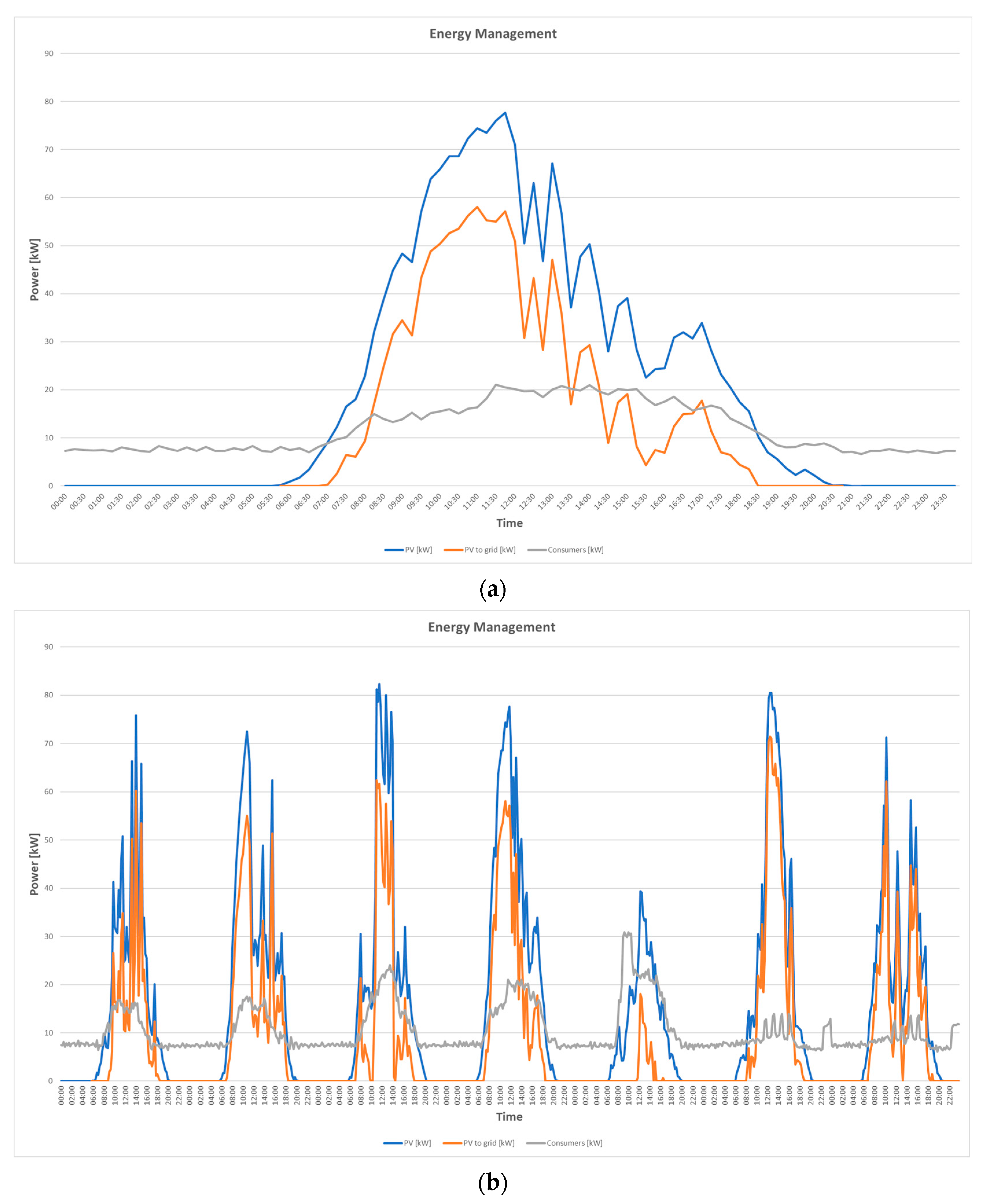
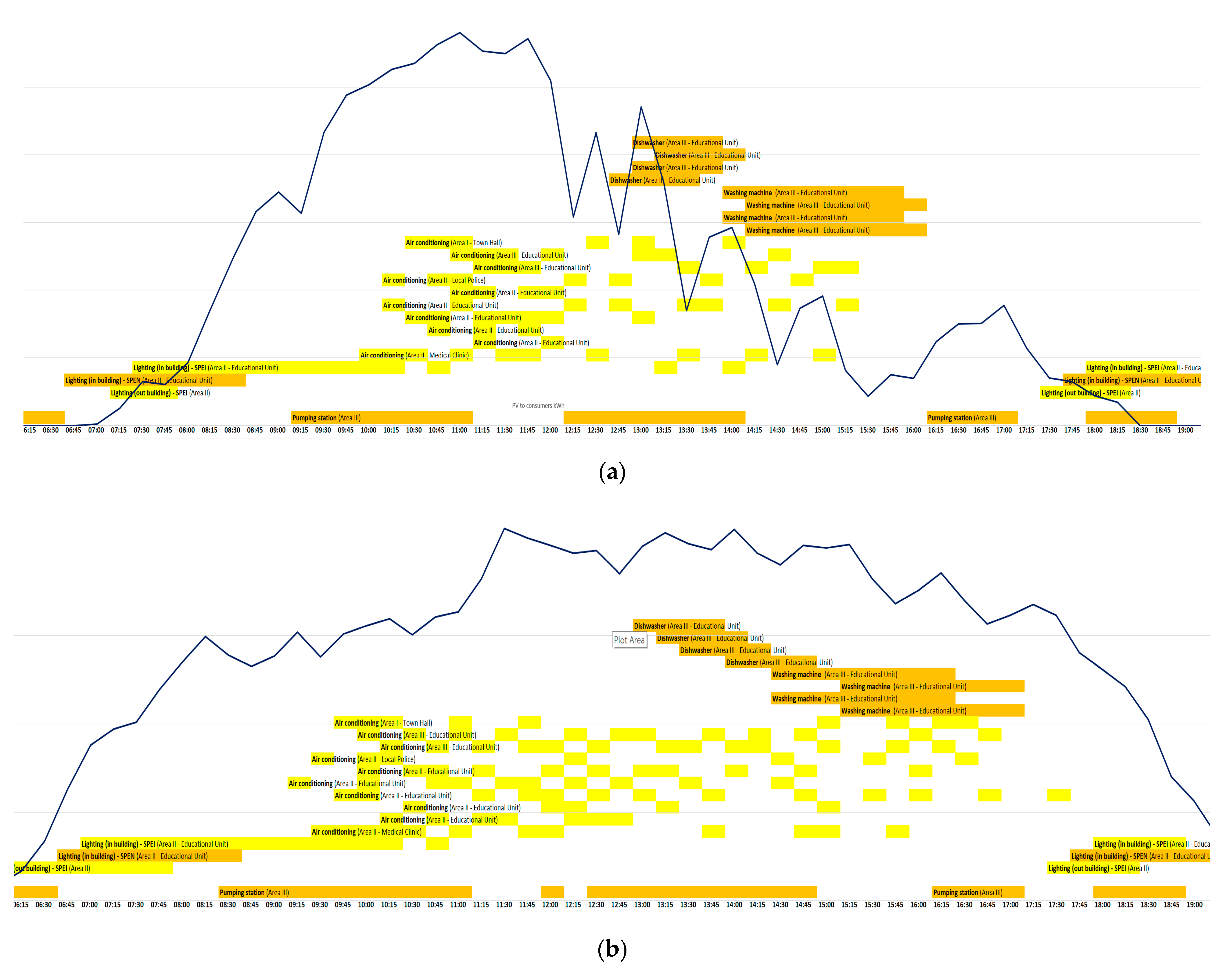
5.2.2. Load Shifting Evaluation

Figure 18a,b show the implementation of the load shifting algorithm on two separate days. Energy-intensive operations of SPE and SPEN appliances were automatically aligned with periods of maximum PV generation, leading to minimized grid dependency and improved local energy self-consumption.

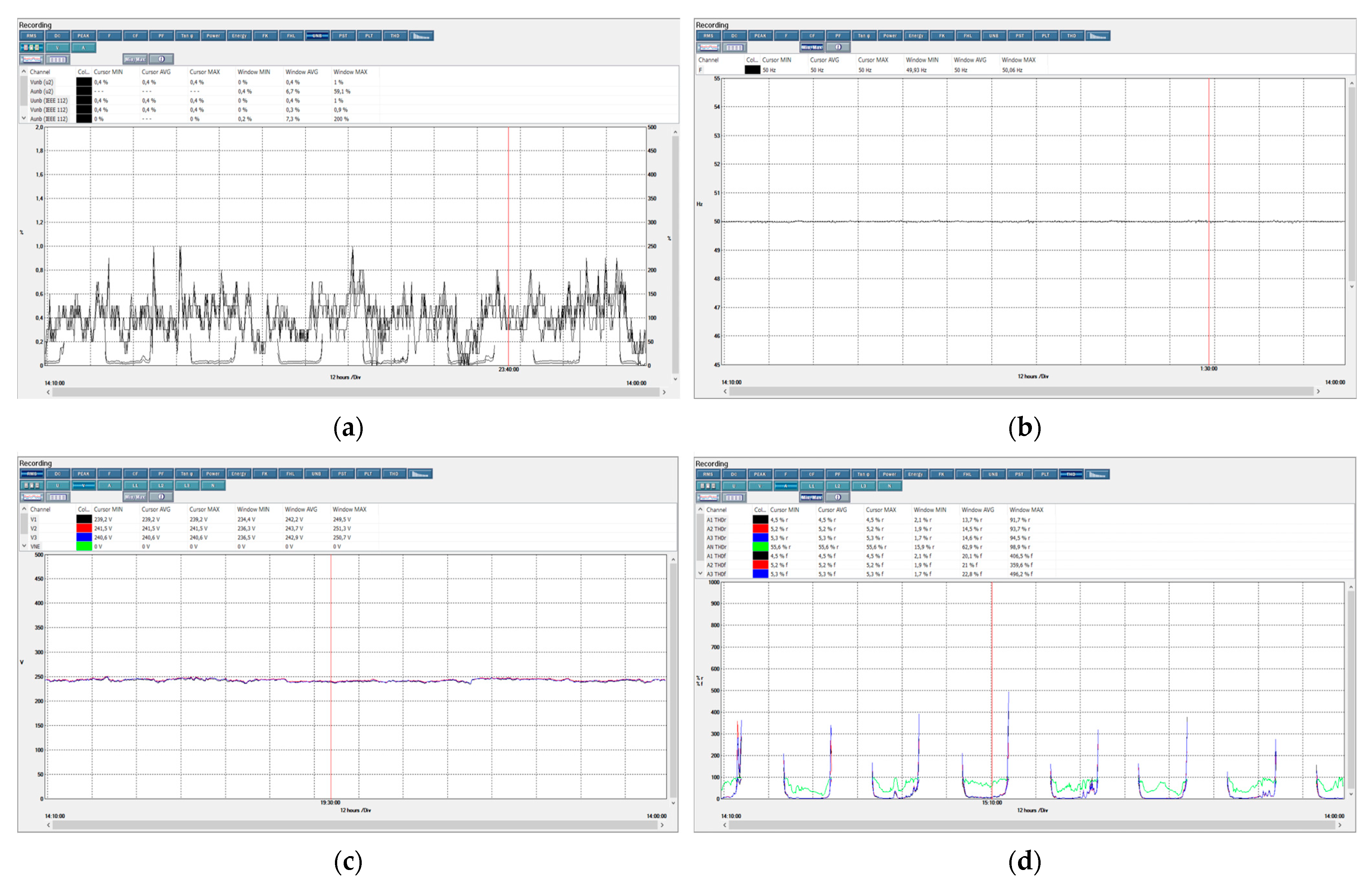
5.2.3. Voltage Quality Assessment

The measurements were carried out using the power quality analyser CA8435 QualistarPlus from Chauvin Arnoux with Power Analyzer Transfer v3.2.0 software, and were performed over a week (11 May 2024, 14:10–15 May 2024, 14:00) on the grid-connected PV system of 83.6 kW in Dambovita, Romania. Such measurements were made for other grid-connected PV systems, and parameter values were obtained that fall within the limits allowed by the quality standards of the produced energy. This analyser is a precise monitoring device that complies with international measurement standards (SR EN 61000-4-30) and can perform measurements according to the limits set by SR EN 50160.

Table 4. Voltage quality standard vs. measured values.

Phenomenon	Standard Values Permissible Limits						Measured Values
Flicker	Plt ≤ 1, for 95% of the week						From Figure 19a–h, we can see that the flicker of the signal in the utility energy grid has a Plt factor of 0.5 and 1.46. From Figure 19a–h, we can see that the flicker of the signal in the utility energy grid has a Plt factor of 0.5 and 1.46. Crucially, the value of Plt also records values greater than 1 for more than 95% of the week, thereby exceeding the permissible standard limit of Plt ≤ 1 for 95% of the week. This deviation is primarily attributed to the hardware construction of converters (which employ switching power electronics) and the inherent power generation dynamics of PV panels.
Fast voltage variations in normal mode	±5% as against nominal voltage Un at low voltage
Unbalanced (negative component)—Kn, to low voltage	Kn ≤ 2%, for 95% of the week; in some areas it may reach 3%;						From Figure 19a, we can see that the frequency of the signal in the utility energy grid has a factor Kn ≤ 1%, for a week. Because of the very low value, we can say that this parameter is within the admissible limits set out in the [25].
Frequency	▪ 50 Hz ± 1% (interconnected grid) ▪ 50 Hz + 4/−6% (isolated grid)						From Figure 19b, we can see that the frequency of the signal in the utility energy grid is within the range 49.93 ÷ 50.06 for a week. Due to the very small variation recorded, we can say that the signal frequency lies within the permissible limits set in the EN 50160 standard.
The nominal frequency of the national energy system is 50 Hz.	▪ 47.00 ÷ 52.00 Hz for 100% per year. ▪ 49.50 ÷ 50.50 Hz for 99.5% per year.
Amplitude of voltage—Average effective value for 10 min of the supplied voltage	in 95% of any time of a week—must not exceed ± 10% of rated nominal voltage at low voltage.						From Figure 19c, we can see that the amplitude of the voltage charged in the utility energy grid is in the range 234.4 V ÷ 249.5 V for phase R, 243.7 V ÷ 251.3 V for phase S, and 242.9 V ÷ 250.7 V for phase T, for a week. Due to the very small variation recorded on the three phases, we can say that this voltage amplitude is within the permissible limits set out in the EN 50160 standard.
Distortion factor for voltage	less than or equal to 8%.						From Figure 19d, we can see that the voltage distortion factor in the utility energy grid is generally less than 8%; however, during the transient operating regimes of the photovoltaic system (start-morning and stop-night), this factor is observed to exceed the standard limit.
Harmonic voltage at boundary points	shall not exceed the maximum limits indicated in the table below for 95% of the week.						From Figure 19e,f, it is observed that the third and fifth odd-numbered harmonics of the currents discharged on the three phases in the utility energy grid are generally less than 5% and 6%, respectively; however, they exceed these limits during the transient operating regimes of the photo-voltaic system. Similarly, other odd and even harmonics generally remain below the allowed limits, except during these transient operating regimes of the photovoltaic system.
	Odd harmonics (% of fundamental):				Even harmonics (%of fundamental):
	Not a multiple of 3		Multiple of 3
	Rank	Limits	Rank	Limits	Rank	Limits
	5	6%	3	5%	2	2%
	7	5%	9	1.5%	4	1%
	11	3.5%	15, 21	0.5%	6 la 24	0.5%
	13	3%
	17	2%
	19, 23, 25	1.5%
Short-term interruptions (shorter than 3 min).	Can range from a few tens to hundreds a year but 70% of them should not last longer than 1 s.						Figure 19g shows that there are not long and short interruptions during the monitored period.
Long-term interruptions (longer than 3 min).	Can be a number from 10 up to 50 per year.
Temporary overvoltage	Cannot exceed 1.5 kV rms for low voltage						From Figure 19h, it is noted that there are no temporary or transient over voltages during the monitored period.
Transitory overvoltage	For low voltage, must be below 6 kV, and can occasionally record even higher values but with a rise time of ms–µs

compares standard limits with measured values.

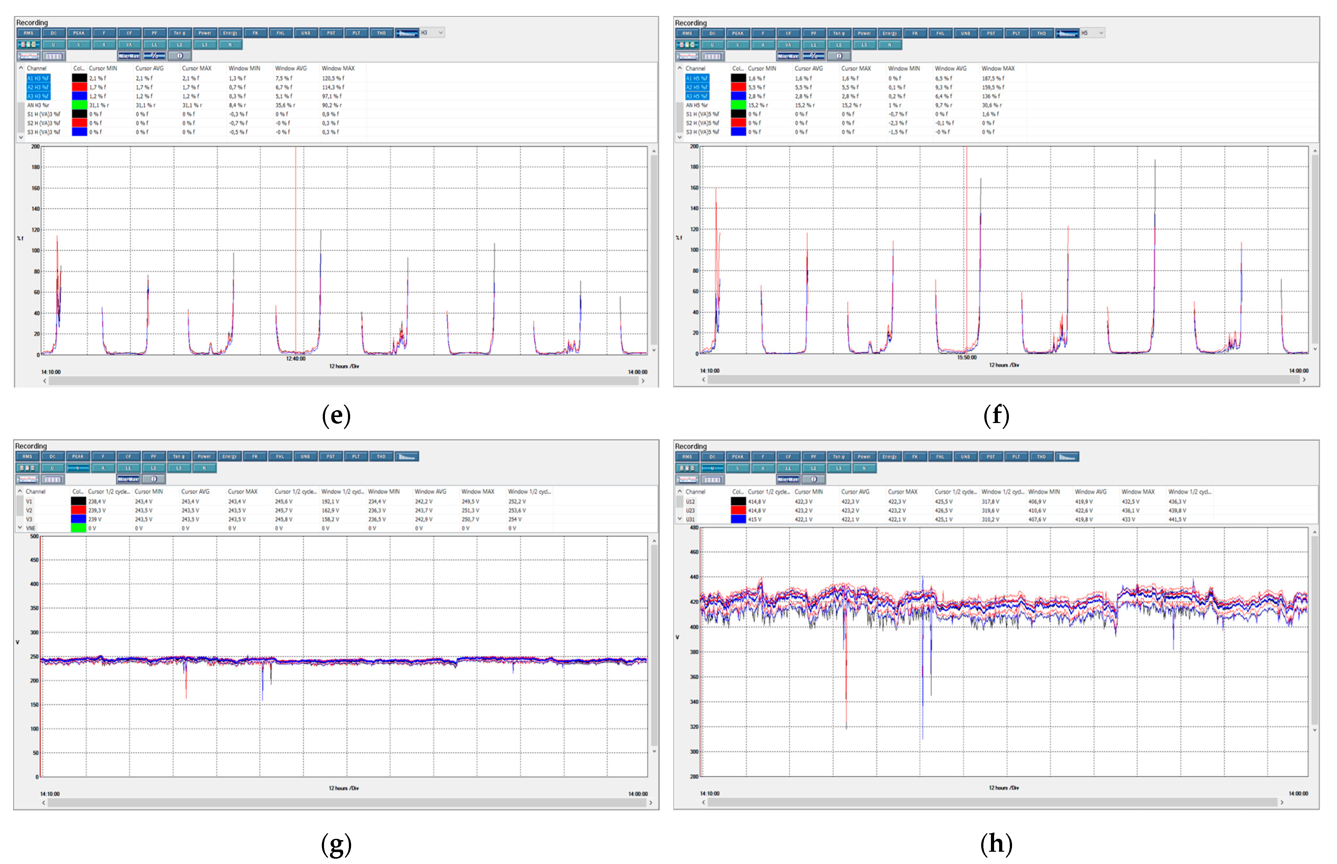
During transient operating regimes, specifically start-morning and stop-night phases, the PV system can introduce significant harmonic distortions. At these times, the voltage distortion factor in the utility grid may exceed 8%, and odd-numbered harmonics (third and fifth) can be higher than standard limits. These harmonics can distort the waveform, negatively impacting electronic devices connected to the grid and potentially leading to malfunctions.

However, the analysis confirms that despite these transient deviations, overall power quality remains within standard limits (SR EN 61000-4-30 and SR EN 50160). The integration of PV systems does not compromise voltage quality when proper inverter controls and grid parameters are maintained. Under normal operating conditions, the influence of PV system harmonics on the load is minimal.

6. Conclusions and Future Work

This paper presents the development of a knowledge-based system that utilizes neuro-fuzzy techniques and intelligent scheduling methods to ensure the optimal use of renewable energy sources (RESs) within a smart grid infrastructure. The main objective was to reduce energy costs incurred by public entities by minimizing their reliance on the national power grid, instead maximizing the use of locally produced green energy through intelligent load management.

The study began by defining the broader context of smart grids integrated with RESs, followed by an analysis of the challenges and opportunities identified in the existing literature. A key focus was placed on managing the energy loads of smart appliances used by public entities. These loads were categorized based on their controllability, operational priority, and the ability to be interrupted—an essential classification for effective load shifting strategies.

The system incorporates a hybrid neuro-fuzzy approach in combination with scheduling algorithms, particularly Mixed-Integer Linear Programming (MILP), enabling predictive modelling based on historical data and real-time meteorological inputs. This allows for dynamic load forecasting, optimal scheduling, and improved local energy self-consumption. The system also includes a robust Maximum Power Point Tracking (MPPT) controller that reliably adapts to environmental changes, ensuring energy efficiency and operational stability.

Experimental validation was carried out on a real infrastructure over several representative days in May 2024. These days were selected based on varying levels of RES energy production and consumption. The results showed that the load shifting algorithm was particularly effective in minimizing grid consumption during periods of low energy production due to unfavourable weather conditions.

Furthermore, the study included a detailed power quality analysis, examining the interaction between harmonics, photovoltaic (PV) systems, and electrical loads. It was observed that while inverters in PV systems can introduce harmonics and flicker due to their switching operations, the overall impact on voltage quality remained within acceptable limits when appropriate inverter controls were implemented. The harmonic distortion was generally low, with most of the distortion influenced more by the nature of the loads than the PV system itself. In particular, harmonics generated by the PV system had a minimal impact on the load, whereas the grid harmonics were significantly affected by load characteristics, especially when inverters operated near their nominal capacity.

The system’s ability to manage loads based on local RES availability not only leads to reduced greenhouse gas emissions but also enhances energy security and self-sufficiency for public institutions. This has direct implications for critical services such as education, healthcare, and local government operations, where stable energy supply is essential.

Although the current implementation is designed primarily for public entities, the framework has clear potential for broader application. In the residential sector, it could be used to lower electricity bills and increase energy independence for households. In the commercial sector, businesses could reduce peak load charges and improve operational efficiency. In the industrial sector, the system could help optimize production cycles in alignment with RES availability, reducing energy costs and environmental impact.

However, the system also presents certain limitations. At this stage, it does not include integration with energy storage systems, and its scalability to other geographic regions and climate conditions remains untested. These aspects are identified as key areas for future research.

Looking forward, ongoing and future work will focus on enhancing the framework by incorporating energy storage systems, enabling multi-objective optimization, and developing scalable models suitable for diverse demographic, institutional, and environmental contexts. Such advancements will further extend the system’s applicability and effectiveness across different sectors.

By combining neuro-fuzzy techniques, advanced scheduling methods, and power quality management, the proposed system provides a practical and scalable solution that supports the global transition to renewable energy. It contributes to sustainable development, reduces the carbon footprint, and promotes resilient energy systems adaptable across a wide range of sectors and communities.