Abstract
In recent years, wireless sensor networks (WSNs) have been employed across various domains, including military services, healthcare, disaster response, industrial automation, and smart infrastructure. Due to the absence of fixed communication infrastructure, WSNs rely on ad hoc connections between sensor nodes to transmit sensed data to target nodes. Within a WSN, a sensor node whose failure partitions the network into disconnected segments is referred to as a critical node or cut vertex. Identifying such nodes is a fundamental step toward ensuring the reliability of WSNs. The critical node detection problem (CNDP) focuses on determining the set of nodes whose removal most significantly affects the network’s connectivity, stability, functionality, robustness, and resilience. CNDP is a significant challenge in network analysis that involves identifying the nodes that have a significant influence on connectivity or centrality measures within a network. However, achieving an optimal solution for the CNDP is often hindered by its time-consuming and computationally intensive nature, especially when dealing with large-scale networks. In response to this challenge, we present a method based on particle swarm optimization (PSO) for the detection of critical nodes. We employ discrete PSO (DPSO) along with the modified position equation (MPE) to effectively solve the CNDP, making it applicable to various k-vertex variations of the problem. We examine the impact of population size on both execution time and result quality. Experimental analysisusing different neighborhood topologies—namely, the star topology and the dynamic topology—was conducted to analyze their impact on solution effectiveness and adaptability to diverse network configurations. We consistently observed better result quality with the dynamic topology compared to the star topology for the same population size, while the star topology exhibited better execution time. Our findings reveal the promising efficacy of the proposed solution in addressing the CNDP, achieving high-quality solutions compared to existing methods.
1. Introduction
A wireless sensor network (WSN) is a distributed, self-organizing wireless system that employs multiple sensor nodes and base stations to monitor various physical or environmental parameters such as temperature, sound, pollution levels, humidity, and wind. WSNs are multi-hop systems made up of many smart sensor nodes and are becoming increasingly common in wireless communication. These nodes are capable of sensing the environment and forwarding data. Each node can gather information for specific applications and help transmit that data to its final destination. This flexible and independent nature makes WSNs well-suited for critical and real-time applications, such as monitoring earthquakes, glacier movements, volcanoes, and forest fires. Massive amounts of data from diverse WSN applications are now being generated. As the scale and importance of WSNs grow, so does the need for adaptable solutions. Ensuring data integrity, accuracy, and reliability is especially crucial in hazardous environments [1]. Sensor nodes play a critical role in WSN-assisted applications that depend on large-scale data transmission [2,3,4,5,6]. However, data communication in WSNs is constrained by the use of ad hoc connections between sensor nodes, which limits scalability and reliability [5,7,8,9].
To address these challenges, recent research has focused on optimization and energy-aware strategies to improve network performance and reliability. For example, an energy-efficient method for cluster head selection based on multiple factors—such as node energy, mobility, queue length, and distance to the cluster center—has shown significant improvements in network lifetime and reduced data loss. This method, combining the cluster splitting process (CSP) with the analytical hierarchy process (AHP), outperforms traditional clustering protocols like BCDCP [10]. Moreover, energy-aware algorithms are not limited to WSNs alone. Similar optimization strategies have been applied to the k-most suitable locations (k-MSL) problem, a facility location issue relevant to WSN deployment planning. By introducing four greedy algorithms, researchers have established an effective baseline for solving the k-MSL problem with real-world relevance in urban and disaster settings [11]. In parallel, sensor systems like LoRaStat further demonstrate the importance of intelligent monitoring solutions. With support for electrochemical sensing and long-term data collection, LoRaStat validates the effectiveness of low-power, high-accuracy monitoring—an essential complement to WSN-based applications, especially in harsh environments [12].
Identifying critical nodes is important in many fields, particularly for improving network security, reliability, and resilience. For example, in the context of enhancing network security, it is essential to identify vulnerabilities, detect critical nodes, monitor them closely, and apply appropriate security measures. These actions help prevent or reduce the impact of attacks and ensure the stable operation of the network [13]. In another example, within network routing, certain nodes are selected to establish the most efficient path between a source and a destination. The security of data traveling through this path depends heavily on the protection of these key nodes. This highlights the importance of the critical node problem in both theoretical and practical contexts. Theoretically, the CNDP is considered an NP-hard problem, meaning it is complex and difficult to solve. In practice, the CNDP has wide-ranging applications in network analysis, including drug development, disease prediction, epidemic control, and identifying key individuals in social or communication networks [14].
One of the significant challenges in WSNs is the identification of critical nodes—also known as cut vertices—whose failure can lead to network fragmentation and the disruption of essential services. These nodes are vital for maintaining the network’s connectivity, stability, centrality, and overall reliability. Therefore, detecting and mitigating the impact of critical nodes is essential for ensuring the resilience and effectiveness of WSN applications.
The CNDP is a well-recognized challenge in network analysis, focused on identifying nodes that have significant influence over a network’s connectivity or centrality measures. These nodes, often referred to as critical nodes, play a crucial role in maintaining the efficiency and resilience of the network. Their failure or malicious manipulation can lead to substantial degradation in network performance.
The CNDP is essentially an optimization task involving the identification of a set of nodes whose removal would result in network disconnection, adversely affecting the functionality of the associated application. Extensive research has been dedicated to addressing the CNDP over the years. Critical nodes are known by various names in the literature, such as key-player nodes [15], most influential nodes [16], k-mediator nodes [17], and most vital nodes [18]. These terms reflect the importance of these nodes in different network contexts. The complexity of the CNDP has been widely studied, with most variants being NP-complete on general graphs, as shown in numerous studies [19,20,21,22]. Additionally, complexity results have been derived for various CNDP variants and graph types [23]. The significance of a node’s criticality in a system depends on the specific configuration adopted upon its removal, a determination influenced by the underlying goals of the application [24,25].
For example, in Figure 1, if the goal is to maximize the number of connected components by removing two nodes, deleting nodes and produces seven components. However, if the goal is to limit each component to at most four nodes, deleting nodes and is optimal. Although both tasks involve deleting nodes, their objectives differ based on the application.
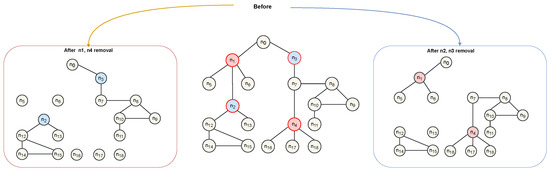
Figure 1.
Illustration of CNDP. The middle panel shows the original network before node removal. The left and right panels depict the network after removing the different sets of critical nodes and , respectively. First scenario: Outer red, inner red: Critical nodes. Outer black, inner yellow: Non-critical nodes. Second scenario: Outer red, inner blue: Critical nodes. Outer black, inner yellow: Non-critical nodes.
Consequently, the significance of a node as critical may vary depending on the perspective taken. Addressing the CNDP often demands substantial computational resources and time, particularly in the context of large-scale networks. To tackle this challenge efficiently, numerous algorithms and methods have been developed. In this study, we propose the utilization of discrete particle swarm optimization (DPSO) as a solution for efficiently solving the CNDP. Particle swarm optimization (PSO), a population-based optimization algorithm, has demonstrated efficacy across diverse optimization problems, owing to its attractive features like simplicity, global search proficiency, robustness, and rapid convergence [26]. PSO is employed in various structural health monitoring applications, serving as a robust and flexible optimization tool that accurately detects structural damage by efficiently exploring the solution space [27].
However, PSO exhibits certain drawbacks, including sensitivity to initial parameters and the tendency to become stuck in local optima. Consequently, careful parameter configuration and exploration of modified or variant algorithms are imperative for achieving the best performance [28].
This paper introduces a novel solution based on DPSO for addressing the challenge of detecting critical nodes. We have conducted experiments using synthetic networks and evaluated the performance using various metrics. Synthetic networks were chosen to provide a controlled environment for testing the proposed method and to assess result sensitivity to different network characteristics. Moreover, it has been observed that certain synthetic networks closely resemble real-world networks. The findings of this study will enrich the literature on the CNDP and offer practical insights for applications requiring the identification of critical nodes in extensive networks. This study thereby contributes to advancing the field of network analysis and offers valuable insights for optimizing critical node detection in diverse networked systems. By developing an efficient algorithm for solving the CNDP in large-scale networks using DPSO, the following specific sub-goals are achieved:
- We propose a novel algorithm utilizing DPSO to address the CNDP. This involves the design, implementation, and comprehensive testing of the algorithm across various network types to ensure its effectiveness and efficiency.
- We evaluate the efficacy of our proposed solution through a comparative analysis with existing techniques that solve CNDP. This assessment includes the use of diverse metrics such as accuracy, speed, and scalability to measure the performance of the algorithm.
- We examine the influence of various parameters on the outcome of the presented algorithm. This assessment includes adjusting different parameters within the algorithm and observing the resultant impact on its performance.
The key abbreviations used in this paper are summarized in Table 1.

Table 1.
Abbreviations.
The remainder of the paper is organized as follows. Section 2 explores related research, while Section 3 provides background information on PSO. Our proposed approach for addressing the CNDP is detailed in Section 4. Section 5 contains a discussion of our findings. Finally, we conclude the paper in Section 6.
2. Related Research
The related work on critical node detection contributes to improving the reliability, resilience, and performance of wireless sensor networks (WSNs). Each study approaches the problem from a different angle—whether it is network structure, optimization techniques, node influence, or algorithm efficiency. This variety helps tackle specific challenges and create solutions that fit the unique needs of different WSN applications. In [29], the angle-based critical node detection (ABCND) algorithm was introduced. It combines 2D critical node detection with RSSI (received signal strength indicator) values from neighboring nodes to improve reliability. However, it does not consider the error rate, which is important for accurate detection in real-world scenarios. The improved TOPSIS method in [30] aimed to identify key nodes based on multiple criteria. While it helped in ranking nodes, it was not efficient in terms of time, making it less suitable for time-sensitive WSN applications. GRASP, a meta-heuristic algorithm, was applied in [31] to find critical nodes in large networks. It focused on improving network reliability, but its accuracy in identifying the most critical nodes was still limited. Two distributed algorithms were proposed in [32] to estimate the state of critical nodes locally within the network. Although this approach reduced the need for centralized processing, it did not solve the issue of high time complexity, which can affect scalability. In [33], a bi-objective approach was introduced to detect critical nodes based on multiple metrics. However, it failed to produce optimized solutions, and simply using multiple metrics did not guarantee more reliable detection. The MCNDI method in [34] used attributes like H-index, closeness centrality, k-shell, and network constraints to rank node importance. Although comprehensive, it lacked timely and accurate detection of key nodes. Similarly, Ref. [35] focused on ranking node importance using structural and performance metrics. Yet, it did not fully address how to detect critical nodes quickly and precisely. The BCVND model in [36] treated critical node detection as a bi-objective problem—aiming to balance connectivity and resource use. However, it struggled to effectively optimize both goals in complex scenarios. An exact iterative algorithm was presented in [37] to detect critical nodes accurately. While precise, this method lacked scalability and efficiency for large-scale WSNs. Reference [38] proposed a new centrality measure called isolating centrality. It was effective in identifying impactful nodes but did not reduce the time required for detection, which limits its usefulness in real-time applications.
In large-scale industrial wireless sensor networks (IWSNs), some nodes are critical for maintaining group-level connectivity. Most previous research on topology control with critical nodes (CNs) has focused only on maintaining connectivity within individual groups. However, ensuring group connectivity without considering these CNs is challenging in group-based IWSNs. Sleep scheduling is a common strategy used to conserve energy in energy-constrained IWSNs while still maintaining connectivity and reliability. Reference [39] proposed a sleep scheduling method that prioritizes critical nodes, allowing them to sleep more than regular nodes to save energy. By preserving the energy of these essential nodes, the network can maintain global connectivity for a longer period.
A cross-layer optimization scheme called adjusting the transmission radius (ATR) was presented in [40]. ATR is built on top of the EC-CKN (energy consumed-uniformly connected k-neighborhood) sleep scheduling algorithm for WSNs. Two key issues in EC-CKN-based networks are identified in [40]: the death acceleration problem and the network isolation problem.
A critical node in a WSN is one whose failure can break the network into disconnected parts, threatening its reliability. Identifying such nodes is essential for maintaining robust network performance. In [41], CDSCUT is introduced as a method based on the connected dominating set, along with five new rules to effectively determine node status and detect critical nodes within the network.
A simple and efficient algorithm called PINC was proposed in [42]. PINC is employed for restoring k-connectivity through node movement. The algorithm classifies nodes into critical (whose failure reduces k-connectivity) and non-critical groups. When a critical node fails, PINC selects a non-critical node—choosing the one that requires the least movement cost—and moves it to the position of the failed node.
Various methods have been implemented in the literature for solving the CNDP, ranging from exact solutions like ILP [19] to various meta-heuristics such as plGA [43], greedy heuristics [19], SA [44], GRASP [31,45], VNS [46], and multi-objective evolutionary algorithms [47]. While exact solutions are available, they are not suitable for solving larger graphs because of the NP-completeness of the problem. Approximation methods, on the other hand, offer practical solutions that may not be optimal but provide good results within a reasonable time frame. Recent solutions have included the addition of machine learning to the set of solutions for node/link criticality detection [23,48]. In [49], authors introduced a population-based memetic algorithm (MemACNP) for solving the CNDP. MemACNP incorporates innovative strategies including node weighting, large component-based node exchange, rank-based pool update, and dual backbone-based crossover. Their study, evaluating 42 scenarios, identified 21 new upper limits and confirmed 18 known higher limits. Additionally, the method was shown effective for the cardinality-constrained CNDP (CC-CNP).
In [50], the authors explored optimal population sizes for memetic algorithms, an area not extensively studied in discrete problem contexts. They introduced variable population memetic search (VPMS), which integrated strategic population sizing (SPS) into the MemA model. VPMS dynamically adjusted the exploration-exploitation balance by incorporating SPS into the standard MemA framework. To enhance exploitation, VPMS initiated a constrained set of two solutions, gradually adding new high-quality solutions to diversify the population. When the population reached its maximum size, VPMS reduced it to two individuals to resume the cycle, aiming to modify the dynamic balance between exploitation and exploration. In [51], the MaxC-GA genetic algorithm addressed the CNDP2a or MaxNum problem, a relatively understudied area. MaxC-GA aimed to minimize the reliance on problem-specific information by encoding the problem in binary and using it solely in the fitness function and constraint management. This has involved representing nodes as “1” for deletion and “0” for retention in the graph. The algorithm has employed two-point crossover and flip-bit mutation, with tournament selection during recombination and mutation. The objective function computed the number of connected components resulting from removing nodes marked as “1” in the binary vector. Test results highlighted MaxC-GA’s superiority over competing algorithms relying more on problem-specific data.
A heuristic technique for addressing the CNDP on planar graphs is presented in [52]. This technique is further investigated in the CC-CNDP, in which the major CNDP target is broken into two sub-goals: maximizing the number of components and minimizing the overall squared difference between component sizes. A method for optimizing these subgoals by selecting appropriate component sizes is described. In contrast, [53] focused on broadening the range of solutions to the weighted CNDP. The approach used two late acceptance strategy-inspired algorithms [54]. The entire strategy, known as iterated local search for NWCNP (ILS-NWCNP) [55], iterated over two complimentary search algorithms, first using a late acceptance technique and then a confined neighborhood local search approach to quickly converge to a locally optimal solution at each iteration. The work in [56] employed the technique of finding key players in networks through deep reinforcement learning in a graph, called FINDER, offering increased customizability and superior solution quality compared to existing approaches. An inductive learning technique using deep-Q network is applied to characterize states and operations in a graph to automatically identify the optimal strategy for achieving the desired objective. Another approach, presented in [57], utilized graph convolutional networks (GCNs) to transform the complex CNDP into a regression problem, resulting in the development of RCNN, which outperforms traditional benchmark methods in spreading dynamics. Additionally, reference [58] formulated the identification of crucial nodes as a binary classification task, using the adjacency matrix and the eigenvector matrix of an influence graph emanated from the initial network structure. While these methodologies exhibit improved performance, they have limitations when applied to real-world problems, such as constraints on network size and reliance on data from the entire graph, making them less applicable to large-scale networks. In [48], a novel graph neural network (GNN) model is introduced for detecting critical nodes or links in large complex networks. Unlike previous methods that focused solely on node influence, this model emphasizes node criticality in terms of its importance to network operation. By producing criticality scores on a small representative portion of the network, the approach enabled accurate predictions for unknown nodes/links in vast graphs while outperforming existing methods in computational efficiency.
However, addressing the CNDP often demands substantial computational resources and time, particularly in the context of large-scale networks. To tackle this challenge efficiently, we propose the utilization of DPSO as a meta-heuristic owing to its efficiency and effectiveness in addressing optimization challenges in large-scale networks.
3. Background: Particle Swarm Optimization
In 1995, Kennedy and Eberhart introduced particle swarm optimization (PSO), inspired by the social interactions of birds seeking food [26]. PSO is a simple and easy-to-implement population-based meta-heuristic technique that imitates birds’ movement within a search space to discover optimal solutions. This makes it a popular preference for solving complex optimization challenges that have multiple resolutions. It is versatile and applicable to various optimization problems in function optimization, machine learning, and control engineering. Despite its strengths in global search capability and escaping local optima depending on the used variant and the used parameters, PSO has limitations like sensitivity to initial parameters and a tendency to get stuck in local optima. Careful parameter setting and algorithm modifications are crucial for achieving optimal performance [28].
The basic form of the PSO algorithm includes two main steps, (i) initialization step and (ii) main iteration as follows:
- Initialization: The particles are initialized with random positions and velocities. Each particle’s personal best location (pbest) is initially set to its current position. The global best position (gbest) is then determined as the best among all personal best locations within the neighborhood.
- Main iteration: The main iteration continues for a specified number of iterations, or until a stop condition is met. It is composed of two steps:
- –
- Movement: The position and velocity of particles are updated as follows:
- –
- Particle’s velocity at iteration :
- –
- Particle’s position at iteration :
- –
- Synchronization: The pbest and gbest positions are updated as follows:
- –
- Compare the present location of the particle to its pbest position and update the pbest location if the current location is better.
- –
- Compare the current location of the particle to the gbest position and update the gbest position if the current location is better.
The components of the velocity update equation can be referred to as follows:
- Inertia: ;
- Cognitive component: ;
- Social component: .
In the equations above, denotes the location of particle i at iteration t, represents its velocity, stands for its personal best position, and indicates the global best position among neighboring particles at iteration t. The acceleration constants are denoted by and , the inertia weight is denoted by w, and denotes a random number between 0 and 1. The balance between global and local search is determined by the inertia weight w. The influence of the personal best and global best positions on velocity update is controlled by and , referred to as cognitive and social coefficients or acceleration factors. The achieved ultimate solution denotes the swarm’s optimal global location.
3.1. Key Factors in Designing a PSO Algorithm
The performance of the particle swarm optimization (PSO) algorithm depends on several key factors that must be carefully considered to achieve optimal results. These factors include the initialization strategy, population size, inertia weight, acceleration coefficients, stopping criteria, velocity clamping, and neighborhood topology. Each plays a critical role in determining the algorithm’s behavior and the quality of the solutions obtained.
In this subsection, we discuss how these factors influence the performance of the PSO algorithm and provide guidelines for selecting them. We also highlight different options for each factor, along with their respective advantages and disadvantages. Understanding the interplay of these factors enables informed decision-making and optimization of the PSO algorithm.
3.1.1. Velocity Clamping
Velocity clamping, introduced by Eberhart and Kennedy [59], prevents particle velocities from diverging by imposing a maximum velocity limit, denoted as . If is too large, particles may move erratically without effectively searching the space; if too small, they may become trapped in local optima. A common approach is to set as , where and are the search space boundaries and typically ranges from 0 to 1.
3.1.2. Population Size
Population size strongly influences the convergence behavior of PSO. A small swarm may inadequately explore the search space, while a large swarm can improve solution quality at the cost of increased computational complexity [60,61]. In practice, population sizes between 20 and 50 are commonly used [62,63,64,65,66]. However, the optimal size depends on the specific problem and the trade-off between exploration and computational resources.
Finding the optimal population size is challenging. One method is sensitivity analysis, which involves running the algorithm with various swarm sizes and analyzing the results [63]. Another approach is dynamic population sizing, which adjusts the swarm size during optimization based on convergence behavior [67].
3.1.3. Initialization Strategy
Initialization has a significant impact on the performance of PSO and other population-based algorithms. While random initialization within the search space is typical, alternative strategies can enhance performance. For example, combining random and heuristic initialization can improve diversity and global search. Warm-start strategies leverage previous solutions, and clustering-based initialization can further boost exploration. However, most of these strategies are general to population-based algorithms rather than specifically designed for PSO. More targeted research is needed for specific applications such as CNDP.
3.1.4. Stopping Criteria
Stopping criteria define when the algorithm terminates. Common choices include a maximum number of iterations or thresholds for changes in the global best position or fitness value. Selecting appropriate stopping criteria is crucial to avoid premature convergence or unnecessary computational effort.
3.1.5. Neighborhood Topology
In PSO, the neighborhood topology determines how particles exchange information, shaping the balance between exploration and exploitation [68].
The star topology (gbest) [26] connects each particle to all others, leading to fast convergence but a higher risk of local optima entrapment. The ring topology (lbest) [68,69] connects each particle to two immediate neighbors, promoting diversity and reducing the risk of local trapping at the expense of slower convergence. The Von Neumann topology connects each particle to its four grid-based neighbors, providing a balance between exploration and exploitation [70].
Dynamic topologies adapt the neighborhood during the search process. For instance, reference [71] suggests starting with limited connections and expanding them over time. DNLPSO [72] also dynamically adjusts neighborhood connections during optimization.
Other topologies include complex [73], hybrid [74], pyramid, wheel, and cluster structures [70,75,76,77].
3.1.6. Inertia Weight and Acceleration Coefficients
The inertia weight governs a particle’s tendency to maintain its current velocity, thus balancing exploration and exploitation. A higher inertia weight encourages exploration, while a lower inertia weight promotes faster convergence to promising regions.
The social and cognitive coefficients, often denoted as and , determine the influence of the personal best and global best solutions, respectively. A higher social coefficient encourages thorough exploration of the search space, while a higher cognitive coefficient steers particles more directly towards known optima.
The choice of inertia weight and acceleration coefficients critically affects the PSO algorithm’s performance. These parameters should be carefully tuned to ensure effective convergence while avoiding local optima entrapment.
4. Proposed Method
The section presents the adaptation of PSO to CNDP using the modified position equation (MPE) method. This adaptation process involves redefining several key components, such as position, velocity, and fitness function, to align with the problem’s specific properties. First, we provide the problem description followed by the PSO discretization approach, dynamic topology design, and finally the operations and topology implementation.
4.1. Problem Description
The CNDP involves removing a subset (along with incident edges) from a graph to satisfy a constraint on a specified metric function f when applied to the residual graph . Typically, network connectivity measures are utilized as metrics. Commonly used metrics include the number of connected components, pairwise connectivity, and giant connected component (GCC) size. The CNDP encompasses various problems based on the metric and constraints on S and f. The problem can be classified into two categories: k-vertex-CNDP and -connectivity-CNDP [23]. The k-vertex-CNDP aims to optimize the metric f while restricting the size of S to a predefined value k (i.e., ). The -connectivity-CNDP seeks to achieve a specific metric value () by minimizing the size of S. We propose a solution suitable to the k-vertex variants of the CNDP, using pairwise connectivity as the metric. Our approach adapts PSO to address this problem effectively.
Pairwise connectivity serves as a useful metric for assessing the connectivity within a graph and identifying the vital nodes for maintaining its overall connectivity. It represents the number of nodes connected through any path and can be calculated as follows:
- We define the connectivity between two nodes as follows:
- The overall pairwise connectivity of a graph is calculated as the summation of the pairwise connectivity between all pairs of nodes in the graph, represented as follows:where V is the graph’s node set.
- The summation of the pairwise connectivity within each connected component is used to determine the overall pairwise connectivity of a graph, as follows:where G is the graph with edges E and nodes V, and is a graph’s connected component. The term indicates the count of nodes in the connected component , and the term represents the number of possible pairs of nodes within the connected component.
4.2. Proposed Adaptive PSO with MPE Method for CNDP
The DPSO algorithm is an adaptation of the classical PSO method, specifically designed for combinatorial optimization problems like CNDP. In CNDP, the objective is to identify a set of k nodes whose removal most significantly disrupts the network’s connectivity. Unlike standard PSO, which operates in continuous space using real-valued vectors for positions and velocities, DPSO deals with discrete solution representations. Each particle in DPSO represents a candidate solution, encoded as a subset of k nodes from the graph. The algorithm begins by initializing a swarm of such particles, each with a random position and a corresponding velocity. The velocity, in this context, is not a vector but rather a mapping function that determines how the current set of nodes should be transformed into a new solution. At each iteration, the DPSO algorithm evaluates the fitness of each particle based on a problem-specific objective function, such as pairwise connectivity, which measures how well connected the network remains after the selected nodes are removed. Each particle retains knowledge of its best solution found so far (pbest) and is also influenced by the best solution found by the entire swarm (gbest). Using these best positions, the particle updates its velocity and position to explore the search space for better solutions. Unlike the numerical updates in traditional PSO, the updates in DPSO are achieved using a set of custom-defined operations under the modified position equation (MPE) framework, which defines how to interpret and manipulate positions and velocities in a discrete setting. The MPE redefines four core PSO operations—position update, velocity subtraction, velocity addition, and scalar multiplication of velocity—to suit the discrete domain. The position plus velocity operation transforms the current solution by applying a mapping function (velocity) to each node in the subset, generating a new node set. The position minus position operation derives the velocity needed to transform one position into another, forming a mapping that captures node swaps. The velocity plus velocity operation combines two such mappings by preserving the non-identity transformations of each and randomly choosing between conflicting changes, simulating the social and cognitive learning components of PSO. Finally, scalar multiplication of a velocity introduces control over the extent of transformation applied. When the scalar is less than or equal to one, only a fraction of the changes defined by the velocity are retained, thus focusing on exploitation. When the scalar is greater than one, random perturbations are introduced to encourage exploration and diversification, mimicking mutation. Together, DPSO and MPE provide a powerful framework for exploring the discrete solution space of CNDP.
In the proposed work, the MPE method is employed to update particle positions in discrete space. This method involves applying discrete operators to the current particle position to generate new solutions appropriate to discrete spaces. Adapting PSO to the CNDP using the MPE method requires redefining key elements such as position, velocity, and fitness function to align with the problem-specific properties. Additionally, the fundamental operations of PSO are redefined to suit the requirements of the CNDP. This adaptation process ensures that PSO can effectively tackle the unique characteristics of the CNDP and its corresponding properties. In this section, we detail the adaptation of PSO to the CNDP using the MPE method. The proposed algorithm is given in Algorithm 1 and is discussed as follows.
Consider a graph, where E is the set of edges, and V is the set of vertices. Our aim is to minimize the pairwise connectivity of the graph by deleting k nodes. We denote for as the graph resulting from deleting the vertices in X and their incident edges from .
- Firstly, we define the position X as a set of k distinct nodes, which will be deleted from the graph. This position indicates a possible solution to the problem and is used by the PSO algorithm to guide its search.
- Secondly, we define the velocity as a permutation of the set of nodes V, where is a bijective function that maps elements of V to other elements of V. The velocity is used by the PSO algorithm to update the position and guide the search toward better solutions.
- Thirdly, we define the objective function as the pairwise connectivity of the graph after the deletion of the nodes in X, where pairwise connectivity represents the count of connected pairs of nodes in the graph. It can be written as , where is the ith connected component in and is the size of the component .
We then define the four operations as follows:
- Position + Velocity, which returns a position as follows. Given a position and a velocity we define,
- Position − Position, which returns a velocity as follows. We define the difference between two positions as , such that, . In other words, if and , we have , we also add the condition that . is the identity function on elements that are not in and for elements that are in . The difference operator is not deterministic and any random solution can be considered
- Velocity + Velocity, which returns a velocity as follows.
- Scalar * Velocity:
- if : Let . Let where is the size of E. We select numbers , where and where with with probability p and 0 otherwise and . Then, can be defined as:
- if : Let . Let , where is the size of E. We select numbers , where, , where, with = 1 with probability p and 0 otherwise, where .Then, can be defined as follows:
Table 2 summarizes the four core operations defined under the MPE framework, which adapt the traditional PSO arithmetic operators to a discrete setting suitable for the CNDP. In this context, a set refers to a particle’s position—that is, a subset of k nodes selected from the graph—while a mapping () denotes a transformation function representing the particle’s velocity. Each operation is reinterpreted to handle these discrete elements, enabling meaningful updates of particle positions within a combinatorial search space.
Table 2.
MPE operations and their purposes.
Additionally, we define the distance between two positions as the number of different elements between the two elements (Hamming distance). In other words, the formula for the distance between two points, X and Y, is .
Algorithm 1 begins by initializing the population of particles and their velocities. It then enters an iterative loop across a set number of generations. In each generation, it evaluates the fitness of each particle (based on pairwise connectivity) and updates the personal best solution (pbest) for each particle and the global best solution (gbest) for the swarm.
For each particle and dimension, it updates the velocity using the MPE framework and executes a series of four specialized operations (referenced in Section 4.2) to refine the position of the particle. It then re-evaluates the fitness of the updated particle and adjusts pbest and gbest if better solutions are found. This process continues until the maximum number of generations is reached, at which point the algorithm returns the best swarm configuration (gbest) with the optimal set of critical nodes identified. Stopping criteria are a crucial component of the PSO algorithm. While many criteria have been proposed in the literature, for this project we focus on two primary stopping criteria. First, we use a convergence criterion to detect when the PSO algorithm reaches a stable solution. Second, we impose a limit on the number of steps to prevent excessive computation if the algorithm fails to converge in a reasonable time frame. Instead of limiting execution time, which can vary depending on hardware and system performance, we limit the number of algorithmic steps. This approach makes our experiments more reproducible. While another common approach is to limit the number of fitness function evaluations, we chose step-based stopping because it is more consistent for our PSO variant, where the number of fitness evaluations per step may vary significantly. To avoid unnecessary computations, we also incorporate an early stopping mechanism that detects convergence before the step limit is reached. Specifically, we define convergence as a situation in which fewer than 10% of the particles continue moving for 10 consecutive steps.
| Algorithm 1 Proposed adaptive PSO with MPE technique for CNDP |
|
4.2.1. Dynamic Topology Design
In PSO, the neighborhood topology refers to how particles exchange information—specifically, how each particle learns about the best solutions found by others. The topology design and operations are discussed as follows: As part of our research, we explored both the star topology and a custom dynamic topology. The dynamic topology is constructed as follows: Initially, we specify a neighborhood size of l. Next, particles are randomly distributed within neighborhoods of size l arranged in a star topology. This arrangement ensures that each particle within the neighborhood has access to the best location of all other particles in the same neighborhood. The technique is then executed for a predetermined number of steps n, after which the neighborhoods are randomly reshuffled, resulting in the regeneration of new neighborhoods of size l. This process continues until the stopping criterion is met. The proposed algorithm for topology design and operations is given in Algorithm 2. Algorithm 2 enhances exploration in PSO by periodically reshuffling neighborhoods, ensuring diverse information sharing and helping avoid premature convergence. The star topology within neighborhoods enables efficient local search between reshuffling steps.
| Algorithm 2 Dynamic neighborhood topology in PSO |
|
4.2.2. Operations and Topology Implementation
The fitness function is calculated using the pairwise connectivity method. The calculation of the pairwise connectivity is executed by searching for connected components, determining their sizes, and then using the formula in Equation (5) to calculate the pairwise connectivity.
The process of finding connected components is conducted through a breadth-first search. The algorithm starts from a node, visits all its neighbors, and then repeats the process for the newly added nodes until all nodes have been visited. If a previously visited node is encountered, we do not re-explore its neighbors. This results in the first connected component. The process is repeated starting from a node that has not been visited to find the newly connected components. This method is continued until every node has been visited.
5. Results and Analysis
The section describes the evaluation framework used for the study, followed by details on the evaluation datasets, results, and analysis. In this work, we evaluate the solutions obtained by the proposed algorithms using two metrics: convergence rate and solution quality. The convergence rate is measured by the execution time required to reach a solution, while the solution quality is assessed by best pairwise connectivity and average pairwise connectivity.
Best Pairwise Connectivity:This refers to the minimum pairwise connectivity achievable in a network after removing the optimal set of critical nodes. It represents the most effective fragmentation of the network, where the fewest pairs of nodes remain connected.
where:
- S is a subset of V (the set of nodes to remove),
- k is the number of nodes to remove,
- if i and j are in the same connected component after removing S, and 0 otherwise.
Average Pairwise Connectivity: This represents the average number of connected pairs across multiple runs of an algorithm or different scenarios. It provides insight into how robust the optimization algorithm is (or how variable the connectivity outcomes are).
where:
- N is the number of experiments or runs,
- is the set of nodes removed in the r-th run.
Execution Time: Execution time indicates how quickly an algorithm or process can solve a problem. For large-scale networks or real-time systems, lower execution time is crucial for feasibility. Execution time reveals how an algorithm’s performance changes as problem size increases.
In this work, we first evaluate the effect of the number of swarms on the solutions generated by the proposed algorithms using the three previously mentioned metrics. We then proceed to compare the solutions obtained by the proposed algorithms to each other. Finally, we compare these solutions to external solutions reported in the literature. It’s worth noting that, when comparing the proposed algorithm to other algorithms in the literature, the best solution is used since most of these works also use the best solution for comparison.
5.1. Test Environment
The algorithm is executed on HPC machines available in the University of Sharjah. More specifically it was run on the FAHAD Cluster characterized by the following. One storage/head node with two Intel Xeon Gold 5120 CPU @ 14Cores—2.20 GHz each, 128 GB RAM and 60 TB Storage. One login node with two Intel Xeon Silver 4110 CPU @ 8Cores—2.10 GHz each and 96 GB RAM. 12 compute nodes with 2 Intel Xeon Gold 6140 CPU @ 18Cores—2.3 GHz each and 192 GB RAM. Each compute node and login node has 240 GB SATA HDD. Mellanox ConnectX-4 Mezzanine card with one EDR/100 Gbps Port. Centos—7.8 operating system and Qlustar-11.0 for cluster management. The compute nodes were used for executing the algorithm. Initially, we executed our algorithm with the default values. The algorithm was coded from scratch using Python 3.8. We executed the algorithm multiple times, varying the population size. Specifically, we ran the algorithm ten times for each population size, except for larger populations in the WS graph, which required more time to execute. For these cases, the algorithm was run one to three times. This approach was taken into account when analyzing the results. Then, we executed the same algorithm a second time with the same parameters with the custom dynamic topology.
5.2. Dataset Details
In our research, we employ a set of 16 benchmark graphs to evaluate the effectiveness of our solution. These graphs, widely recognized in the field and publicly accessible, provide a standardized benchmark for evaluating solutions to the CNDP, facilitating equitable comparisons between different approaches. These graphs are organized into sets of four, each set consisting of graphs generated using the same model but varying in size. Specifically, the 16 graphs are generated based on the models of Watts–Strogatz, Erdos–Reni, Forest Fire, and Barabasi–Albert [23]. Table 3 provides an overview of the evaluation dataset.
Table 3.
Evaluation dataset.
5.2.1. Erdős–Rényi Model
The Erdős–Rényi (ER) model generates random graphs by connecting each pair of nodes with a fixed probability p. It is useful for studying random structures and has a Poisson degree distribution. However, it is not well-suited for modeling real-world networks, which typically follow a power-law distribution. Figure 2 shows an example Erdős–Rényi random graph with 235 vertices and 349 edges.
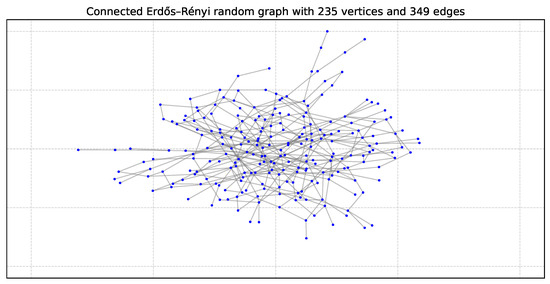
Figure 2.
Graph ER235: Erdős–Rényi random graph with 235 vertices and 349 edges [44].
5.2.2. Barabási–Albert Model
The Barabási–Albert (BA) model simulates network growth using preferential attachment: new nodes are more likely to connect to existing nodes with higher degrees. This leads to a power-law degree distribution, a common feature in real-world networks. Figure 3 shows an example Barabási–Albert graph with 1000 vertices.
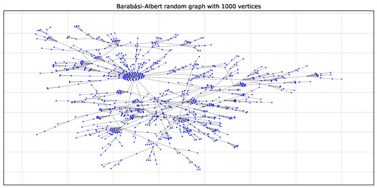
Figure 3.
Graph BA1000: Barabási–Albert random graph with 1000 vertices [44].
At each step, a new node connects to m existing nodes with probability:
5.2.3. Watts–Strogatz Model
The Watts–Strogatz (WS) model generates small-world networks. It starts with a regular ring lattice and rewires some edges randomly. The result is a graph with high clustering and short path lengths, similar to many real-world systems such as social or communication networks. Figure 4 shows an example Watts–Strogatz small world model with 250 vertices.
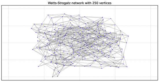
Figure 4.
Graph WS250: Watts–Strogatz network with 250 vertices [44].
5.2.4. Forest Fire Model
The Forest Fire model also uses preferential attachment but produces graphs with scale-free properties and shrinking diameter over time. It begins with a few seed nodes and adds new ones, which connect to existing nodes probabilistically. This results in a heavy-tailed degree distribution where a few nodes have many connections, and most have few. Figure 5 shows an example of a Forest Fire graph.
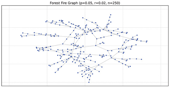
Figure 5.
Graph FF250: Forest Fire random graph model with a forward probability of and a backward probability of , respectively [44].
5.3. Analysis Using a Star Topology
We run the program with the star topology and random initialization for values of , = , and = . We run the program for different population sizes from 50 to 102,400 in order to analyze the effect of PSO adapted to CNDP with a main focus on the population size. For each population size, the program is run 10 times to see the impact of the randomness of the technique.
5.3.1. Comparison: Quality of the Results
Figure 6, Figure 7, Figure 8 and Figure 9 show the average minimum pairwise connectivity and the best pairwise connectivity over 10 runs as a function of the population size for each of the benchmark graphs. The graphs are plotted on a logarithmic scale to make them easily readable.
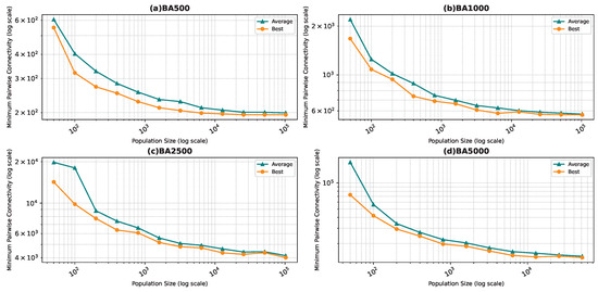
Figure 6.
Best and average pairwise connectivity as a function of the population size for the star topology: Barabási–Albert model.
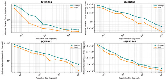
Figure 7.
Best and average pairwise connectivity as a function of the population size for the star topology: Erdős–Rényi model.
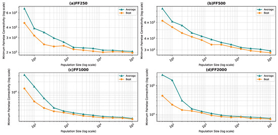
Figure 8.
Best and average pairwise connectivity as a function of the population size for the star topology: Forest Fire model.
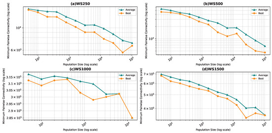
Figure 9.
Best and average pairwise connectivity as a function of the population size for the star topology: Watts–Strogatz model.
In all the figures, we observe a trend where bigger population sizes lead to improved result quality. However, a distinct pattern emerges for the smallest graphs, particularly those generated by the BA and FF models, where the marginal improvements reduce for larger population sizes. This phenomenon is attributed to the inherent features of these graphs, which display a “rich get richer” pattern during generation, making it easier to identify critical nodes with significant impact on pairwise connectivity, especially with smaller populations. Similarly, smaller graphs inherently demand smaller populations to yield satisfactory results. Conversely, for ER and WS graphs, larger populations consistently improve result quality, indicating the greater complexity of the problem and the tendency of the method to experience local minima or divergence. Notably, the WS algorithm often fails to converge before fulfilling the stopping criteria, while the ER algorithm tends to become trapped in local minima.
We also notice that the average and best values become closer to each other as we use more particles. This is justified by the fact that the algorithm starts avoiding local minima, and thus all runs find almost the best results. This is not true for the graphs ER and WS since the number of particles we achieved is not enough to avoid local optima in both cases. For ER1000, ER2500, and WS1000, WS1500 graphs, we notice that the gap between the two graphs is not that big. This is mainly due to the fact that we only ran the algorithm around three times, and we could not do more since the time each run takes is very high, especially for the WS graphs, where the algorithm does not converge before the step limit.
5.3.2. Comparison: Execution Time
One would assume that the quality of the result will improve with growing populations. However, this comes at a cost. We observe that the computation time grows linearly with the population size, while the quality improvement is not linear. Thus, it is important to keep a logical population size as a compromise between computation time and the quality of the result. We noticed some anomalies with the WS graphs, which are the most challenging graphs due to their construction. It is very hard to discover the optimal solution because the solution space is full of local optima. Generally, we noticed that the program rarely converges for these graphs before the stop condition, thus the execution time is large. We also noticed anomalies when convergence happens due to a lucky seed.
Figure 10, Figure 11, Figure 12 and Figure 13 show the execution time as a function of the population size for the star topology.
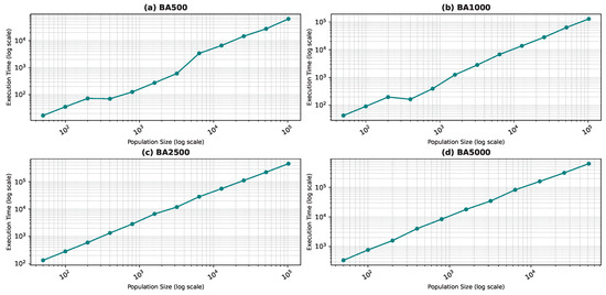
Figure 10.
Execution time as a function of the population size for the star topology: Barabási–Albert model.
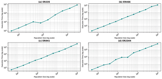
Figure 11.
Execution time as a function of the population size for the star topology: Erdős–Rényi model.
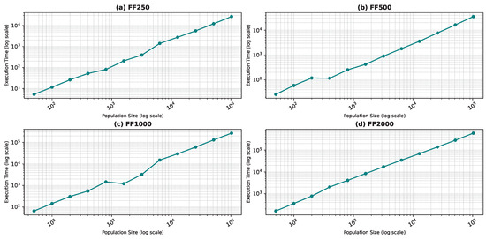
Figure 12.
Execution time as a function of the population size for the star topology: Forest Fire model.
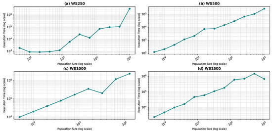
Figure 13.
Execution time as a function of the population size for the star topology: Watts–Strogatz model.
In Figure 13d, the execution time unexpectedly decreases for the largest population size (100,000). This may be due to faster convergence in highly connected swarms at large scales or due to hardware-level parallel processing optimizations that are better utilized at larger scales. Furthermore, in the WS1500 scenario, the structure of the neighborhoods might allow faster convergence at larger sizes because more diverse or “globa” information is accessible to the particles.
5.4. Analysis Using a Dynamic Topology
This section discusses the analysis using dynamic topology. We run the algorithm using the custom dynamic topology described earlier in Section 4.2.1 with values and .
5.4.1. Comparison: Quality of the Results
Figure 14, Figure 15, Figure 16 and Figure 17 show the average minimum pairwise connectivity and the best pairwise connectivity over 10 runs as a function of the population size for each of the benchmark graphs in both the dynamic and the star topology. The graphs are plotted on a logarithmic scale for better understanding. We denote the dynamic topology as “D” and the star topology as “S” in the graph’s legend.
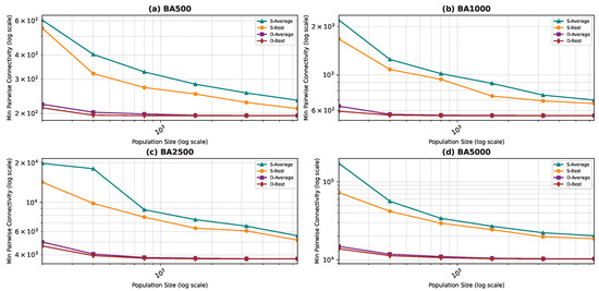
Figure 14.
Best and average pairwise connectivity as a function of the population size comparison between the star topology and the dynamic topology: Barabási–Albert model.
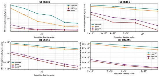
Figure 15.
Best and average pairwise connectivity as a function of the population size comparison between the star topology and the dynamic topology: Erdős–Rényi model.
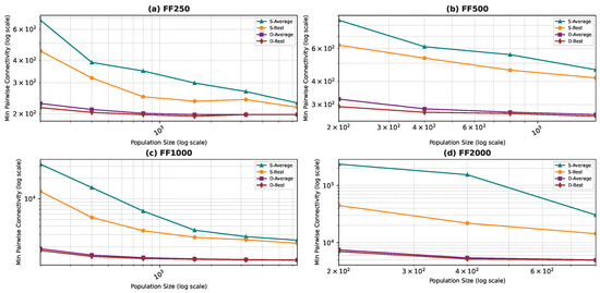
Figure 16.
Best and average pairwise connectivity as a function of the population size comparison between the star topology and the dynamic topology: Forest Fire model.
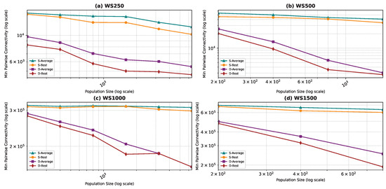
Figure 17.
Best and average pairwise connectivity as a function of the population size comparison between the star topology and the dynamic topology: Watts–Strogatz model.
Similar to the star topology, we observed that increasing the population size generally improves results for the dynamic topology. However, we also noted that for smaller and simpler graphs, such as BA and FF graphs, the improvement in results plateaus at a certain population size. In fact, for these graphs, we even attained near-optimal solutions that closely match or approach the best possible outcomes generated by exact methods documented in the literature, as detailed in Table 4 in Section 5.5. Furthermore, upon comparing the dynamic topology to the star topology, we found that the dynamic topology requires a smaller population size to achieve superior results. In many instances, the dynamic topology outperformed the star topology with a smaller population size for all population sizes. Additionally, we consistently observed better pairwise connectivity with the dynamic topology for the same population size. We observed better pairwise connectivity with the dynamic topology for the same population size. This is due to the fact that our dynamic topology transforms standard PSO into a dynamic neighborhood-based PSO that adaptively balances local exploitation and global exploration, leading to a more robust and effective search process—particularly for complex optimization problems. The fixed-period reshuffling ensures periodic exposure to new neighborhoods, while still exploiting the local best within each neighborhood in between. This fixed-interval, random reshuffling after n steps—combined with the star topology within neighborhoods—strikes a unique balance between exploration (new neighborhoods) and exploitation (star-based local best search).
Table 4.
Comparison of the best value (minimum pairwise connectivity achieved) found by our solutions with those reported in other papers.
5.4.2. Comparison: Execution Time
Figure 18, Figure 19, Figure 20 and Figure 21 illustrate the relationship between population size and execution time for both algorithms. The trends observed for the star topology remain consistent across most graphs, with the exception of BA500 and FF250, which are the least complex graphs in the dataset. Interestingly, for these graphs, we notice a decline in execution time beyond a certain population size, contrary to the expected trend. We postulate that a larger population size increases the likelihood of some particles initializing in advantageous positions, thereby reducing the convergence steps. However, this hypothesis necessitates further validation through an examination of the particles’ movement history, which was not recorded in our study. Nevertheless, our preliminary analysis of the raw data confirms the observed decrease in convergence steps. In the case of graphs generated using the WS model, the linear pattern of the results is not maintained. Due to the problem’s complexity, we believe that the number of particles used in the algorithm is much smaller than required, leading to convergence issues. When checking the raw data, we found that the algorithm rarely converged except a few times resulting in a sudden decrease in execution time.
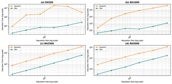
Figure 18.
Execution time as a function of the population size comparison between the star topology and the dynamic topology: Barabási–Albert model.
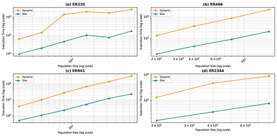
Figure 19.
Execution time as a function of the population size comparison between the star topology and the dynamic topology: Erdős–Rényi model.
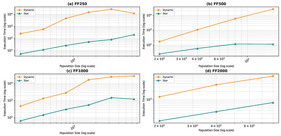
Figure 20.
Execution time as a function of the population size comparison between the star topology and the dynamic topology: Forest Fire model.
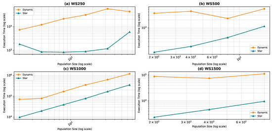
Figure 21.
Execution time as a function of the population size comparison between the star topology and the Dynamic topology: Watts–Strogatz model.
Comparing the two topologies, we found that the dynamic topology is significantly slower than the star topology. This result was expected, as our objective in introducing the dynamic topology was to enhance exploration at the cost of exploitation. It is worth noting that in Figure 18, Figure 19, Figure 20 and Figure 21, the population size is limited in the range of 200–6400, even though we ran the algorithm for the star topology for smaller and larger population sizes. We chose to limit the population size to ensure graph visibility. In fact, for the dynamic topology, we could not run the algorithm for larger populations due to time constraints.
5.5. Discussion
We compare the performance of our solutions for identifying critical nodes in various graph models to the results reported in the survey conducted by LALOU et al. [23], covering only the results published prior to 2018. We summarize the comparison outcomes in Table 4.
Our solution employing the star topology is denoted as PSOS, while our dynamic topology solution is labeled as PSOD. We select the best results obtained across all population sizes for each graph. Remarkably, our algorithm produced notably favorable outcomes, particularly with PSOD, for graphs generated using the Barabási-Albert and Forest Fire models, which are inherently simpler problems due to their few highly connected nodes. Furthermore, we achieved improved results with PSOD on smaller graphs, particularly with the challenging WS graphs, which pose difficulties in identifying critical nodes. With the exception of WS1500, our results ranked among the best reported in the literature, despite running the algorithm only a few times for these graphs due to the complexity of finding solutions. While increasing the population size could potentially enhance overall results, our primary focus is on refining the algorithm itself and other relevant parameters to achieve efficiency. Notably, PSO offers several adjustable parameters that significantly influence execution time and result quality, and although we have explored only a subset of these elements, further investigation holds promise for achieving even better outcomes. Conversely, we observed poor results for the ER940, ER2343, and WS1500 graphs. It is difficult to justify this observation; however, we can say that we stopped at a small population size for these graphs due to execution time constraints.
5.6. Results Summary
Our solution employing the star topology is denoted as PSOS, while our dynamic topology solution is labeled as PSOD. In contrast to existing approaches, the study by [44] introduced simulated annealing (SA) and population-based incremental learning (PBIL) methods for addressing the critical node detection problem. Building upon these ideas, our framework integrates the variable neighborhood search (VNS) methodology [78] and incorporates strategies from greedy algorithms and local search, similar to the approaches in [79]. Moreover, two metaheuristics grounded in the iterated local search (ILS) and VNS frameworks were explored in [46], further advancing the field. A comparison of our proposed methods (PSOS and PSOD) with these established algorithms is provided in Table 4. This table highlights the best values obtained by our algorithms alongside those reported in the literature for PBIL, SA, VNS, GrdA, and ILS, showcasing the competitiveness and effectiveness of our approach in the critical node detection domain.
Figure 14, Figure 15, Figure 16, Figure 17, Figure 18, Figure 19, Figure 20 and Figure 21 reveal key differences between the dynamic topology (PSOD) and the static star topology (PSOS) across the four benchmark network models: Barabási–Albert (BA), Erdős–Rényi (ER), Forest Fire (FF), and Watts–Strogatz (WS).
Best and Average Connectivity: Across all models, PSOD consistently achieves lower best and average pairwise connectivity values than PSOS. This confirms that the dynamic topology is more effective at identifying critical nodes that fragment the network.
Variance of Solutions: PSOD also exhibits lower variance across multiple runs, suggesting more reliable and stable performance—particularly valuable in critical applications such as infrastructure and sensor networks.
Execution Time: These performance gains come at the cost of higher execution time in PSOD, due to its adaptive neighborhood updates and increased search complexity.
Model-Specific Insights:
- Barabási–Albert (BA): PSOD shows the most dramatic improvements, with up to 90% lower connectivity than PSOS. The scale-free structure of BA networks allows PSOD to exploit hub removal effectively.
- Erdős–Rényi (ER): Randomly connected ER graphs also benefit from dynamic topologies, as redundant paths can be more effectively disrupted by PSOD.
- Forest Fire (FF): FF graphs’ community-like structures are particularly well-suited to PSOD’s flexible search, resulting in significantly lower average and best connectivity.
- Watts–Strogatz (WS): WS networks follow a similar trend due to PSOD’s adaptability to clustered, short-path structures.
- Across all graph types, the dynamic topology (PSOD) consistently achieves a lower average and best pairwise connectivity compared to the star topology (PSOS).
- This advantage is especially pronounced in larger graphs (e.g., BA5000, FF2000) where dynamic updates to neighborhood topology enable more effective identification of critical nodes.
- Despite these gains, the dynamic topology requires higher execution times, reflecting the added computational overhead of dynamically adapting the neighborhood structure during the optimization process.
- The variance in connectivity measures is typically lower in the dynamic topology, suggesting more stable and consistent performance across runs.
- The dynamic topology’s enhanced ability to adapt to local network structures significantly improves the effectiveness of critical node detection, reducing connectivity far beyond the static star topology baseline. Although, this comes at the cost of higher computation time, the trade-off is justified in scenarios where robustness and minimization of network connectivity are paramount—such as in wireless sensor networks and other dynamic environments.
- While PSOD incurs additional computational costs, it consistently delivers superior solutions—achieving lower connectivity, reduced variance, and better adaptation to local network structures. The improvements are especially pronounced in larger BA and FF networks, underscoring the importance of dynamic search topologies in complex, heterogeneous network environments.
6. Conclusions
In this study, we have adapted the PSO algorithm to address the CNDP, which involves the identification of critical nodes within a large-scale network. Our approach introduces an MPE method that maps the operations and fitness function to the problem at hand. We have also tested our solution using carefully chosen stopping criteria and parameter values. One of the major challenges in using PSO for critical node detection is determining the appropriate population size and neighborhood topology. We investigated the influence of population size on solution quality and execution time. We have also explored two different neighborhood topologies—a star topology and a custom dynamic topology. Our results show that the dynamic neighborhood topology achieved better results, even though the execution time was slower. Overall, our findings suggest that the proposed method is a viable approach to the CNDP. Our results show that careful parameter tuning and adaptation have resulted in high-quality solutions that are competitive with existing approaches. To evaluate the applicability and efficiency of our solution to other CNDP variants, a detailed analysis is required, and we consider this as future work. In particular, we aim to adapt the PSOD algorithm with the MPE technique for dynamic networks, making it responsive to environmental changes and capable of maintaining solution relevance. A key enhancement involves introducing a time-varying fitness function, allowing particles to be evaluated based on the current network topology. Additionally, a dynamic velocity scaling mechanism will be implemented by adjusting the scalar multiplier within the MPE framework—promoting exploration when the network changes and encouraging exploitation as it stabilizes. To further maintain diversity and prevent premature convergence, especially after major network shifts, new particles can be introduced into the swarm either randomly or using heuristics such as node centrality. These enhancements are expected to make the PSOD-MPE framework more robust, flexible, and effective in real-time or evolving network environments, with potential applications in mobile networks, dynamic infrastructure systems, and adaptive security planning. Moreover, in future experiments, we aim to test the proposed approach on publicly available datasets such as road networks, airline routes, or online social graphs to further validate its generalizability and practical utility.
Author Contributions
Conceptualization, A.M., W.O., B.A. and A.M.K.; methodology, B.A. and A.M.K.; software, A.M. and W.O.; validation, A.M., W.O., B.A. and A.M.K.; formal analysis, A.M., W.O., B.A. and A.M.K.; investigation, A.M., W.O. and A.M.K.; data curation, A.M. and W.O.; writing—original draft preparation, A.M. and W.O.; writing—review and editing, B.A. and A.M.K.; visualization, W.O.; supervision, A.M.K.; project administration, B.A.; funding acquisition, B.A. All authors have read and agreed to the published version of the manuscript.
Funding
This research received no external funding.
Institutional Review Board Statement
Not applicable.
Informed Consent Statement
Not applicable.
Data Availability Statement
The original contributions presented in this study are included in the article.
Acknowledgments
The researchers would like to thank the Deanship of Graduate Studies and Scientific Research at Qassim University for financial support (QU-APC-2025).
Conflicts of Interest
The authors declare no conflicts of interest.
References
- Adday, G.H.; Subramaniam, S.K.; Zukarnain, Z.A.; Samian, N. Fault Tolerance Structures in Wireless Sensor Networks (WSNs): Survey, Classification, and Future Directions. Sensors 2022, 22, 6041. [Google Scholar] [CrossRef] [PubMed]
- Khedr, A.M.; Ramadan, H. Effective sensor relocation technique in mobile sensor networks. Int. J. Comput. Netw. Commun. (IJCNC) 2011, 3, 204–217. [Google Scholar] [CrossRef]
- Khedr, A.M.; Osamy, W. Minimum connected cover of a query region in heterogeneous wireless sensor networks. Inf. Sci. 2013, 223, 153–163. [Google Scholar] [CrossRef]
- Khedr, A.M.; Omar, D.M. SEP-CS: Effective Routing Protocol for Heterogeneous Wireless Sensor Networks. Ad Hoc Sens. Wirel. Netw. 2015, 26, 211–234. [Google Scholar]
- Omar, D.M.; Khedr, A.M.; Agrawal, D.P. Optimized clustering protocol for balancing energy in wireless sensor networks. Int. J. Commun. Netw. Inf. Secur. 2017, 9, 367–375. [Google Scholar] [CrossRef]
- Salim, A.; Osamy, W.; Khedr, A.M.; Aziz, A.; Abdel-Mageed, M. A secure data gathering scheme based on properties of primes and compressive sensing for IoT-based WSNs. IEEE Sens. J. 2020, 21, 5553–5571. [Google Scholar] [CrossRef]
- Khedr, A.M.; Osamy, W. Mobility-assisted minimum connected cover in a wireless sensor network. J. Parallel Distrib. Comput. 2012, 72, 827–837. [Google Scholar] [CrossRef]
- Osamy, W.; Khedr, A.M. An algorithm for enhancing coverage and network lifetime in cluster-based wireless sensor networks. Int. J. Commun. Netw. Inf. Secur. 2018, 10, 1–9. [Google Scholar] [CrossRef]
- Aziz, A.; Singh, K.; Osamy, W.; Khedr, A.M. An efficient compressive sensing routing scheme for internet of things based wireless sensor networks. Wirel. Pers. Commun. 2020, 114, 1905–1925. [Google Scholar] [CrossRef]
- Rahiminasab, A.; Tirandazi, P.; Ebadi, M.; Ahmadian, A.; Salimi, M. An energy-aware method for selecting cluster heads in wireless sensor networks. Appl. Sci. 2020, 10, 7886. [Google Scholar] [CrossRef]
- Mirghaderi, S.H.; Hassanizadeh, B. k-most suitable locations problem: Greedy search approach. Int. J. Ind. Syst. Eng. 2022, 42, 80–95. [Google Scholar] [CrossRef]
- Amngostar, P.; Dehabadi, M.; Hagh, S.F.; Badireddy, A.R.; Huston, D.; Xia, T. LoRaStat: A Low-cost Portable LoRaWAN Potentiostat for Wireless and Real-Time Monitoring of Water Quality and Pollution. IEEE Sens. J. 2024, 25, 1561–1570. [Google Scholar] [CrossRef]
- Hamouda, E. A critical node-centric approach to enhancing network security. In Proceedings of the International Conference on the Dynamics of Information Systems, Prague, Czech Republic, 3–6 September 2023; Springer: Berlin/Heidelberg, Germany, 2023; pp. 116–130. [Google Scholar]
- Liu, C.; Ge, S.; Chen, Z.; Pei, W.; Zhu, E.; Mei, Y.; Ishibuchi, H. Improving Critical Node Detection Using Neural Network-based Initialization in a Genetic algorithm. arXiv 2024, arXiv:2402.00404. [Google Scholar]
- Corley, H.; Sha, D.Y. Most vital links and nodes in weighted networks. Oper. Res. Lett. 1982, 1, 157–160. [Google Scholar] [CrossRef]
- Kempe, D.; Kleinberg, J.; Tardos, É. Influential Nodes in a Diffusion Model for Social Networks. In Proceedings of the Automata, Languages and Programming, Lisbon, Portugal, 11–15 July 2005; Caires, L., Italiano, G.F., Monteiro, L., Palamidessi, C., Yung, M., Eds.; Springer: Berlin/Heidelberg, Germany, 2005; pp. 1127–1138. [Google Scholar]
- Li, C.T.; Lin, S.D.; Shan, M.K. Finding Influential Mediators in Social Networks. In Proceedings of the 20th International Conference Companion on World Wide Web, Hyderabad, India, 28 March–1 April 2011; Association for Computing Machinery: New York, NY, USA, 2011; pp. 75–76. [Google Scholar] [CrossRef]
- Borgatti, S.P. Identifying sets of key players in a social network. Comput. Math. Organ. Theory 2006, 12, 21–34. [Google Scholar] [CrossRef]
- Arulselvan, A.; Commander, C.W.; Elefteriadou, L.; Pardalos, P.M. Detecting critical nodes in sparse graphs. Comput. Oper. Res. 2009, 36, 2193–2200. [Google Scholar] [CrossRef]
- Shen, S.; Smith, J.C.; Goli, R. Exact interdiction models and algorithms for disconnecting networks via node deletions. Discret. Optim. 2012, 9, 172–188. [Google Scholar] [CrossRef]
- Berger, A.; Grigoriev, A.; van der Zwaan, R. Complexity and approximability of the k-way vertex cut. Networks 2014, 63, 170–178. [Google Scholar] [CrossRef]
- Arulselvan, A.; Commander, C.W.; Shylo, O.; Pardalos, P.M. Cardinality-Constrained Critical Node Detection Problem. In Performance Models and Risk Management in Communications Systems; Springer: New York, NY, USA, 2011; pp. 79–91. [Google Scholar] [CrossRef]
- Lalou, M.; Tahraoui, M.A.; Kheddouci, H. The Critical Node Detection Problem in networks: A survey. Comput. Sci. Rev. 2018, 28, 92–117. [Google Scholar] [CrossRef]
- Wang, M.; Xiang, Y.; Wang, L. Identification of critical contingencies using solution space pruning and intelligent search. Electr. Power Syst. Res. 2017, 149, 220–229. [Google Scholar] [CrossRef]
- Veremyev, A.; Pavlikov, K.; Pasiliao, E.L.; Thai, M.T.; Boginski, V. Critical nodes in interdependent networks with deterministic and probabilistic cascading failures. J. Glob. Optim. 2019, 74, 803–838. [Google Scholar] [CrossRef]
- Kennedy, J.; Eberhart, R. Particle swarm optimization. In Proceedings of the ICNN’95—International Conference on Neural Networks, Perth, WA, Australia, 27 November–1 December 1995; Volume 4, pp. 1942–1948. [Google Scholar] [CrossRef]
- Mazloom, S.; Rabbani, A.; Rahami, H.; Sa’adati, N. A Two-Stage Damage Localization and Quantification Method in Trusses Using Optimization Methods and Artificial Neural Network by Modal Features. Iran. J. Sci. Technol. Trans. Civ. Eng. 2024, 1–18. [Google Scholar] [CrossRef]
- Clerc, M.; Kennedy, J. The particle swarm—Explosion, stability, and convergence in a multidimensional complex space. IEEE Trans. Evol. Comput. 2002, 6, 58–73. [Google Scholar] [CrossRef]
- Shukla, S. Angle Based Critical Nodes Detection (ABCND) for Reliable Industrial Wireless Sensor Networks. Wirel. Pers. Commun. 2023, 130, 757–775. [Google Scholar] [CrossRef]
- Liu, L.; Wang, W.; Jiang, G.; Zhang, J. Identifying Key Node in Multi-region Opportunistic Sensor Network based on Improved TOPSIS. Comput. Sci. Inf. Syst. 2021, 18, 19. [Google Scholar] [CrossRef]
- Sembroiz, D.; Ojaghi, B.; Careglio, D.; Ricciardi, S. A GRASP Meta-Heuristic for Evaluating the Latency and Lifetime Impact of Critical Nodes in Large Wireless Sensor Networks. Sensors 2019, 9, 4564. [Google Scholar] [CrossRef]
- Dagdeviren, O.; Akram, V.K.; Tavli, B. Design and Evaluation of Algorithms for Energy Efficient and Complete Determination of Critical Nodes for Wireless Sensor Network Reliability. IEEE Trans. Reliab. 2019, 68, 280–290. [Google Scholar] [CrossRef]
- Li, J.; Pardalos, P.M.; Xin, B.; Chen, J. The bi-objective critical node detection problem with minimum pairwise connectivity and cost: Theory and algorithms. Methodol. Appl. 2019, 23, 12729–12744. [Google Scholar] [CrossRef]
- Zhang, Y.; Lu, Y.; Yang, G.; Hang, Z. Multi-Attribute Decision Making Method for Node Importance Metric in Complex Network. Appl. Sci. 2022, 12, 1944. [Google Scholar] [CrossRef]
- Yin, R.; Yin, X.; Cui, M.; Xu, Y. Node importance evaluation method based on multi-attribute decision-making model in wireless sensor networks. EURASIP J. Wirel. Commun. Netw. 2019, 234. [Google Scholar] [CrossRef]
- Zhang, L.; Xia, J.; Cheng, F.; Qiu, J.; Zhang, X. Multi-Objective Optimization of Critical Node Detection Based on Cascade Model in Complex Networks. IEEE Trans. Netw. Sci. Eng. 2020, 7, 2052–2066. [Google Scholar] [CrossRef]
- Rezaei, J.; Zare-Mirakabad, F.; MirHassani, S.A.; Marashi, S.A. EIA-CNDP: An exact iterative algorithm for critical node detection problem. Comput. Oper. Res. 2021, 127, 105138. [Google Scholar] [CrossRef]
- Ugurlu, O. Comparative analysis of centrality measures for identifying critical nodes in complex networks. J. Comput. Sci. 2022, 62, 101738. [Google Scholar] [CrossRef]
- Wang, D.; Mukherjee, M.; Shu, L.; Chen, Y.; Hancke, G. Sleep scheduling for critical nodes in group-based industrial wireless sensor networks. In Proceedings of the 2017 IEEE International Conference on Communications Workshops (ICC Workshops), Paris, France, 21–25 May 2017; pp. 694–698. [Google Scholar] [CrossRef]
- Shu, L.; Wang, L.; Niu, J.; Zhu, C.; Mukherjee, M. Releasing Network Isolation Problem in Group-Based Industrial Wireless Sensor Networks. IEEE Syst. J. 2017, 11, 1340–1350. [Google Scholar] [CrossRef]
- Dagdeviren, O.; Akram, V.K.; Tavli, B.; Yildiz, H.U.; Atilgan, C. Distributed detection of critical nodes in wireless sensor networks using connected dominating set. In Proceedings of the 2016 IEEE SENSORS, Orlando, FL, USA, 30 October–3 November 2016; pp. 1–3. [Google Scholar] [CrossRef]
- Khalilpour Akram, V.; Akusta Dagdeviren, Z.; Dagdeviren, O.; Challenger, M. PINC: Pickup Non-Critical Node Based k-Connectivity Restoration in Wireless Sensor Networks. Sensors 2021, 21, 6418. [Google Scholar] [CrossRef]
- Aringhieri, R.; Grosso, A.; Hosteins, P.; Scatamacchia, R. A general Evolutionary Framework for different classes of Critical Node Problems. Eng. Appl. Artif. Intell. 2016, 55, 128–145. [Google Scholar] [CrossRef]
- Ventresca, M. Global search algorithms using a combinatorial unranking-based problem representation for the critical node detection problem. Comput. Oper. Res. 2012, 39, 2763–2775. [Google Scholar] [CrossRef]
- Purevsuren, D.; Cui, G.; Win, N.N.H.; Wang, X. Heuristic algorithm for identifying critical nodes in graphs. Adv. Comput. Sci. Int. J. 2016, 5, 1–4. [Google Scholar]
- Aringhieri, R.; Grosso, A.; Hosteins, P.; Scatamacchia, R. Local search metaheuristics for the critical node problem. Networks 2016, 67, 209–221. [Google Scholar] [CrossRef]
- Ventresca, M.; Harrison, K.R.; Ombuki-Berman, B.M. An Experimental Evaluation of Multi-objective Evolutionary Algorithms for Detecting Critical Nodes in Complex Networks. In Proceedings of the Applications of Evolutionary Computation, Copenhagen, Denmark, 8–10 April 2015; Mora, A.M., Squillero, G., Eds.; Springer: Cham, Switzerland, 2015; pp. 164–176. [Google Scholar]
- Munikoti, S.; Das, L.; Natarajan, B. Scalable graph neural network-based framework for identifying critical nodes and links in complex networks. Neurocomputing 2022, 468, 211–221. [Google Scholar] [CrossRef]
- Zhou, Y.; Hao, J.K.; Glover, F. Memetic Search for Identifying Critical Nodes in Sparse Graphs. IEEE Trans. Cybern. 2019, 49, 3699–3712. [Google Scholar] [CrossRef] [PubMed]
- Zhou, Y.; Hao, J.K.; Fu, Z.H.; Wang, Z.; Lai, X. Variable Population Memetic Search: A Case Study on the Critical Node Problem. IEEE Trans. Evol. Comput. 2021, 25, 187–200. [Google Scholar] [CrossRef]
- Zhang, X.; Duan, F.; Zhang, L.; Cheng, F.; Jin, Y.; Tang, K. Pattern Recommendation in Task-oriented Applications: A Multi-Objective Perspective [Application Notes]. IEEE Comput. Intell. Mag. 2017, 12, 43–53. [Google Scholar] [CrossRef]
- Purevsuren, D.; Cui, G. Efficient heuristic algorithm for identifying critical nodes in planar networks. Comput. Oper. Res. 2019, 106, 143–153. [Google Scholar] [CrossRef]
- Zhou, Y.; Wang, Z.; Jin, Y.; Fu, Z.H. Late acceptance-based heuristic algorithms for identifying critical nodes of weighted graphs. Knowl.-Based Syst. 2021, 211, 106562. [Google Scholar] [CrossRef]
- Burke, E.K.; Bykov, Y. A late acceptance strategy in hill-climbing for exam timetabling problems. In Proceedings of the PATAT 2008 Conference, Montreal, QC, Canada, 18–22 August 2008; pp. 1–7. [Google Scholar]
- Lourenço, H.R.; Martin, O.C.; Stützle, T. Iterated Local Search: Framework and Applications. In Handbook of Metaheuristics; Springer International Publishing: Cham, Switzerland, 2019; pp. 129–168. [Google Scholar] [CrossRef]
- Fan, C.; Zeng, L.; Sun, Y.; Liu, Y.Y. Finding key players in complex networks through deep reinforcement learning. Nat. Mach. Intell. 2020, 2, 317–324. [Google Scholar] [CrossRef]
- Yu, E.Y.; Wang, Y.P.; Fu, Y.; Chen, D.B.; Xie, M. Identifying critical nodes in complex networks via graph convolutional networks. Knowl.-Based Syst. 2020, 198, 105893. [Google Scholar] [CrossRef]
- Sun, M.; Jiang, Y.; Wang, Y.; Xie, H.; Wang, Z. Identification of Critical Nodes in Dynamic Systems Based on Graph Convolutional Networks. In Proceedings of the 2020 3rd International Conference on Unmanned Systems (ICUS), Harbin, China, 27–28 November 2020; pp. 558–563. [Google Scholar] [CrossRef]
- Eberhart, R.C.; Dobbins, R.W.; Hutton, L.V. Neural network paradigm comparisons for appendicitis diagnoses. In Proceedings of the Computer-Based Medical Systems-Proceedings of the Fourth Annual IEEE Symposium, Baltimore, MD, USA, 12–14 May 1991; pp. 298–299. [Google Scholar]
- Bergh, F.V.D.; Engelbrecht, A.P. Effects of Swarm Size on Cooperative Particle Swarm Optimisers. In Proceedings of the 3rd Annual Conference on Genetic and Evolutionary Computation, San Francisco, CA, USA, 7–11 July 2001; pp. 892–899. [Google Scholar]
- Himanshu, N.; Burman, A. Determination of Critical Failure Surface of Slopes Using Particle Swarm Optimization Technique Considering Seepage and Seismic Loading. Geotech. Geol. Eng. 2019, 37, 1261–1281. [Google Scholar] [CrossRef]
- Chen, W.N.; Zhang, J.; Lin, Y.; Chen, N.; Zhan, Z.H.; Chung, H.S.H.; Li, Y.; Shi, Y.H. Particle Swarm Optimization With an Aging Leader and Challengers. IEEE Trans. Evol. Comput. 2013, 17, 241–258. [Google Scholar] [CrossRef]
- Piotrowski, A.P.; Napiorkowski, J.J.; Piotrowska, A.E. Population size in Particle Swarm Optimization. Swarm Evol. Comput. 2020, 58, 100718. [Google Scholar] [CrossRef]
- Wang, D.; Tan, D.; Liu, L. Particle swarm optimization algorithm: An overview. Soft Comput. 2018, 22, 387–408. [Google Scholar] [CrossRef]
- Ratnaweera, A.; Halgamuge, S.; Watson, H. Self-organizing hierarchical particle swarm optimizer with time-varying acceleration coefficients. IEEE Trans. Evol. Comput. 2004, 8, 240–255. [Google Scholar] [CrossRef]
- Beheshti, Z.; Hj. Shamsuddin, S.M. CAPSO: Centripetal accelerated particle swarm optimization. Inf. Sci. 2014, 258, 54–79. [Google Scholar] [CrossRef]
- Rangasamy, D.P.; Rajappan, S.; Natarajan, A.; Ramasamy, R.; Vijayakumar, D. Variable population-sized particle swarm optimization for highly imbalanced dataset classification. Comput. Intell. 2021, 37, 873–890. [Google Scholar] [CrossRef]
- Kennedy, J. Small worlds and mega-minds: Effects of neighborhood topology on particle swarm performance. In Proceedings of the 1999 Congress on Evolutionary Computation-CEC99 (Cat. No. 99TH8406), Washington, DC, USA, 6–9 July 1999; Volume 3, pp. 1931–1938. [Google Scholar] [CrossRef]
- Mendes, R.; Kennedy, J.; Neves, J. The fully informed particle swarm: Simpler, maybe better. IEEE Trans. Evol. Comput. 2004, 8, 204–210. [Google Scholar] [CrossRef]
- Kennedy, J.; Mendes, R. Population structure and particle swarm performance. In Proceedings of the 2002 Congress on Evolutionary Computation. CEC’02 (Cat. No. 02TH8600), Honolulu, HI, USA, 12–17 May 2002; Volume 2, pp. 1671–1676. [Google Scholar] [CrossRef]
- Suganthan, P. Particle swarm optimiser with neighbourhood operator. In Proceedings of the 1999 Congress on Evolutionary Computation-CEC99 (Cat. No. 99TH8406), Washington, DC, USA, 6–9 July 1999; Volume 3, pp. 1958–1962. [Google Scholar] [CrossRef]
- Nasir, M.; Das, S.; Maity, D.; Sengupta, S.; Halder, U.; Suganthan, P. A dynamic neighborhood learning based particle swarm optimizer for global numerical optimization. Inf. Sci. 2012, 209, 16–36. [Google Scholar] [CrossRef]
- Godoy, A.; Von Zuben, F.J. A Complex Neighborhood based Particle Swarm Optimization. In Proceedings of the 2009 IEEE Congress on Evolutionary Computation, Trondheim, Norway, 18–21 May 2009; pp. 720–727. [Google Scholar] [CrossRef]
- Zhang, L.; Yu, H.; Hu, S. A New Approach to Improve Particle Swarm Optimization. In Proceedings of the Genetic and Evolutionary Computation—GECCO 2003, Chicago, IL, USA, 12–16 July 2003; Cantú-Paz, E., Foster, J.A., Deb, K., Davis, L.D., Roy, R., O’Reilly, U.M., Beyer, H.G., Standish, R., Kendall, G., Wilson, S., et al., Eds.; Springer: Berlin/Heidelberg, Germany, 2003; pp. 134–139. [Google Scholar]
- Part Introduction. In Computational Intelligence; John Wiley & Sons, Ltd.: Hoboken, NJ, USA, 2007; pp. 285–287. [CrossRef]
- Mendes, R.; Kennedy, J.; Neves, J. Watch thy neighbor or how the swarm can learn from its environment. In Proceedings of the 2003 IEEE Swarm Intelligence Symposium. SIS’03 (Cat. No.03EX706), Indianapolis, IN, USA, 26 April 2003; pp. 88–94. [Google Scholar] [CrossRef]
- Xu, Y.; Pi, D. A reinforcement learning-based communication topology in particle swarm optimization. Neural Comput. Appl. 2020, 32, 10007–10032. [Google Scholar] [CrossRef]
- Aringhieri, R.; Grosso, A.; Hosteins, P.; Scatamacchia, R. VNS solutions for the Critical Node Problem. Electron. Notes Discret. Math. 2015, 47, 37–44. [Google Scholar] [CrossRef]
- Addis, B.; Aringhieri, R.; Grosso, A.; Hosteins, P. Hybrid constructive heuristics for the critical node problem. Ann. Oper. Res. 2016, 238, 637–649. [Google Scholar] [CrossRef]
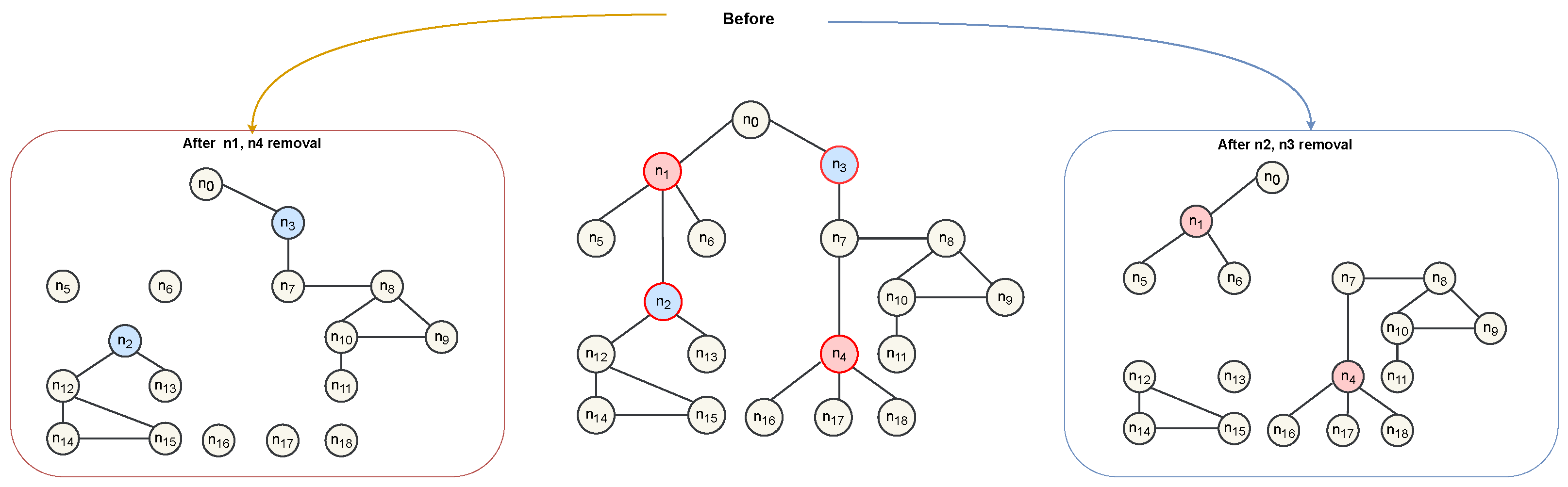
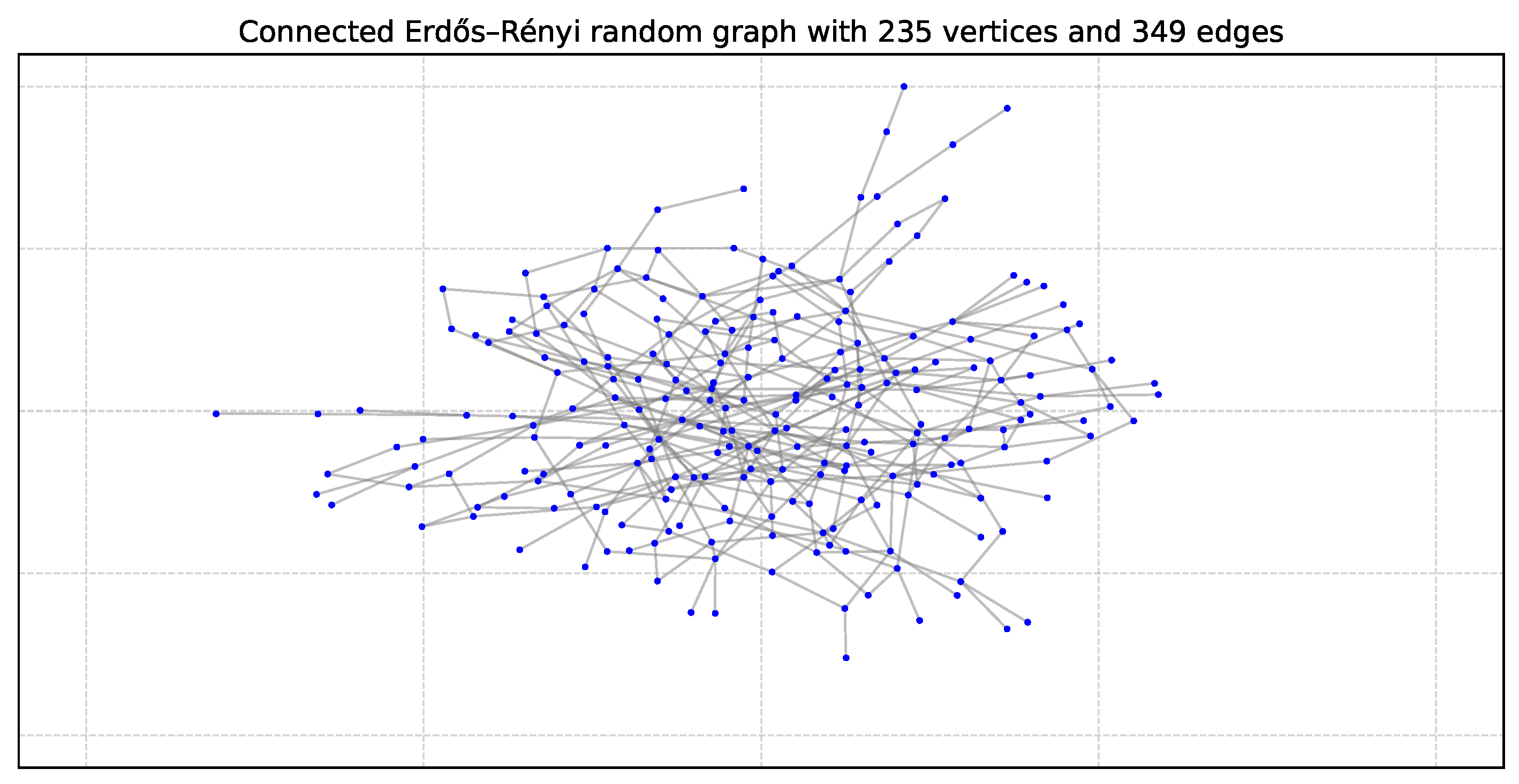

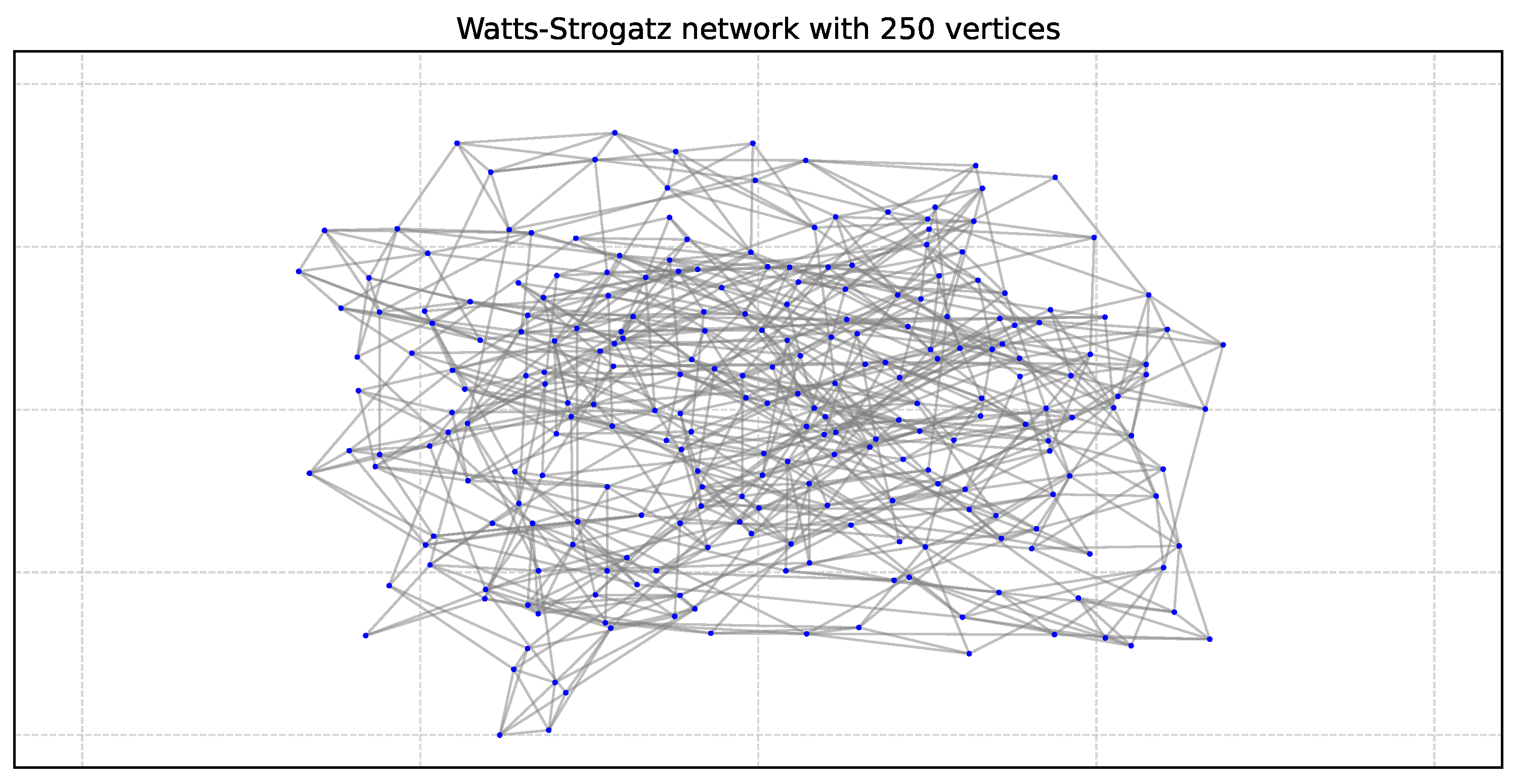
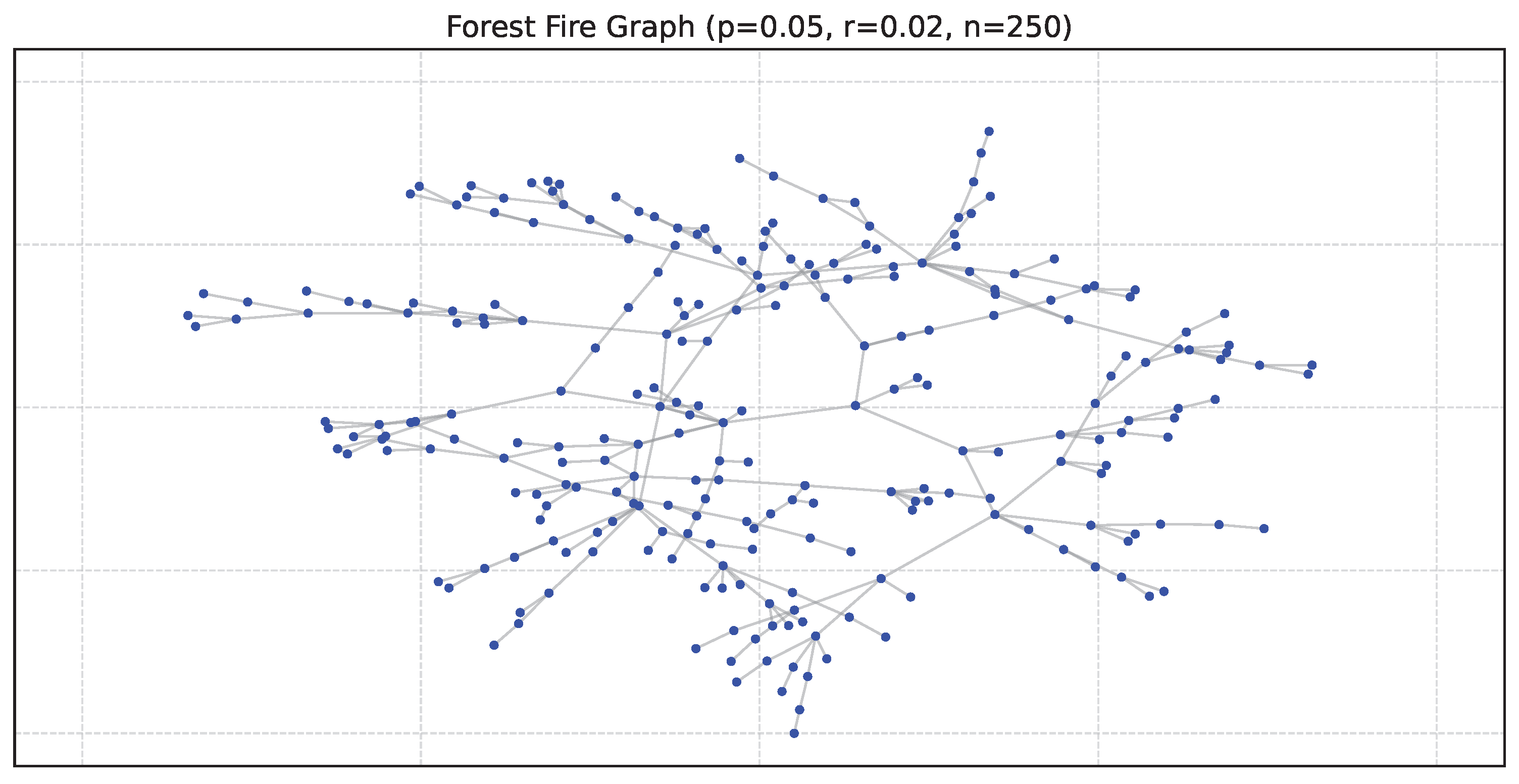
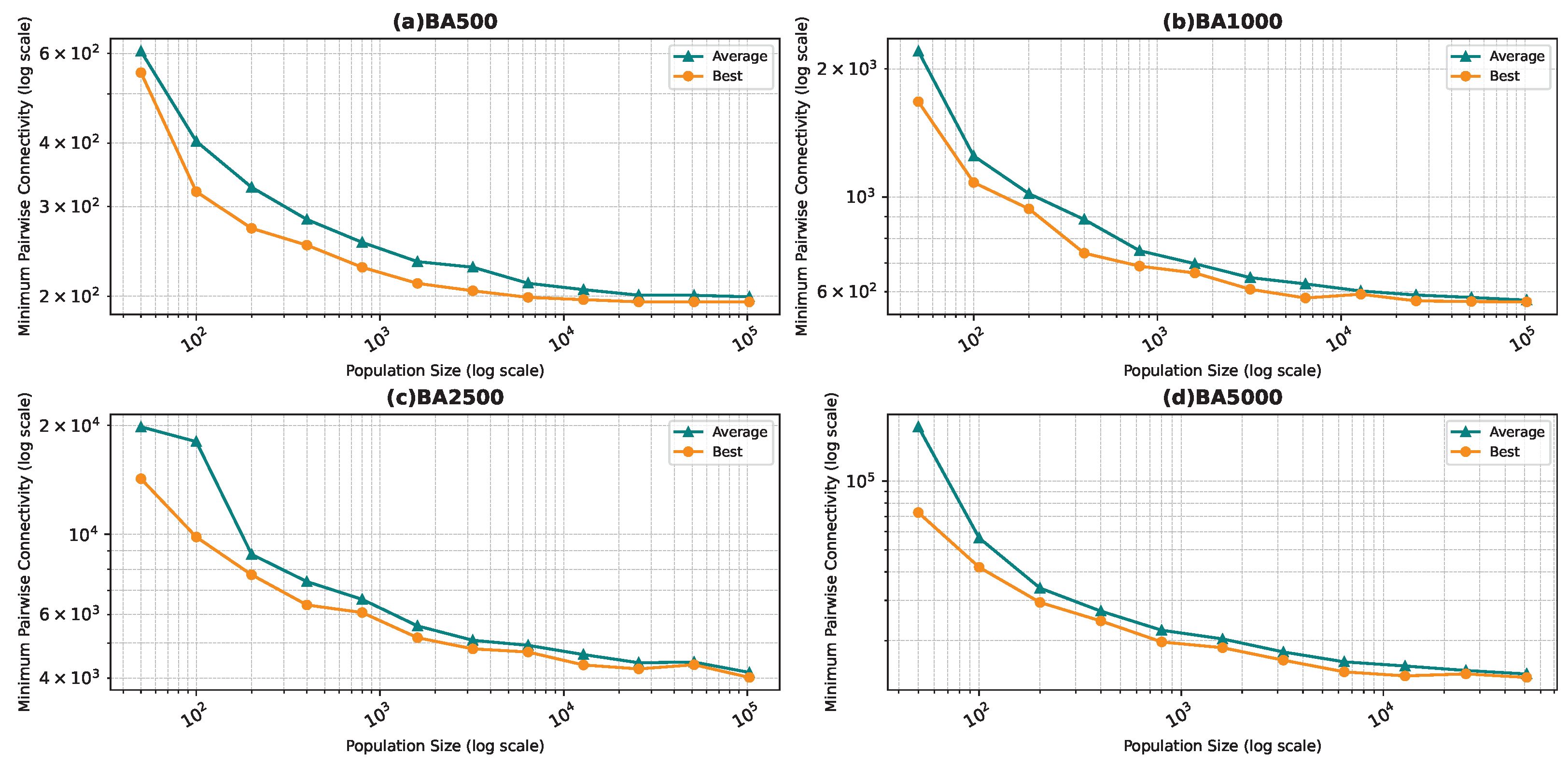
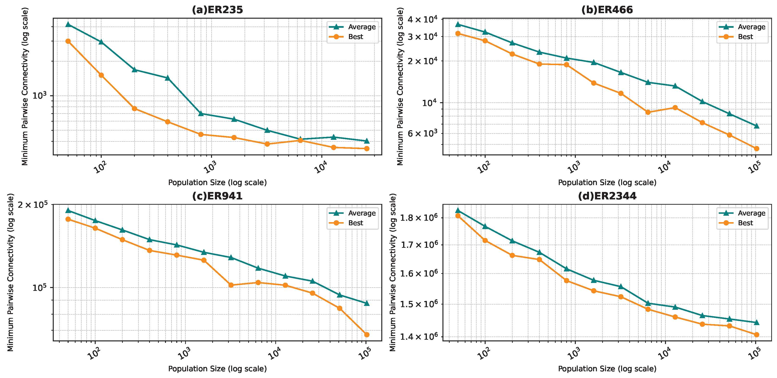
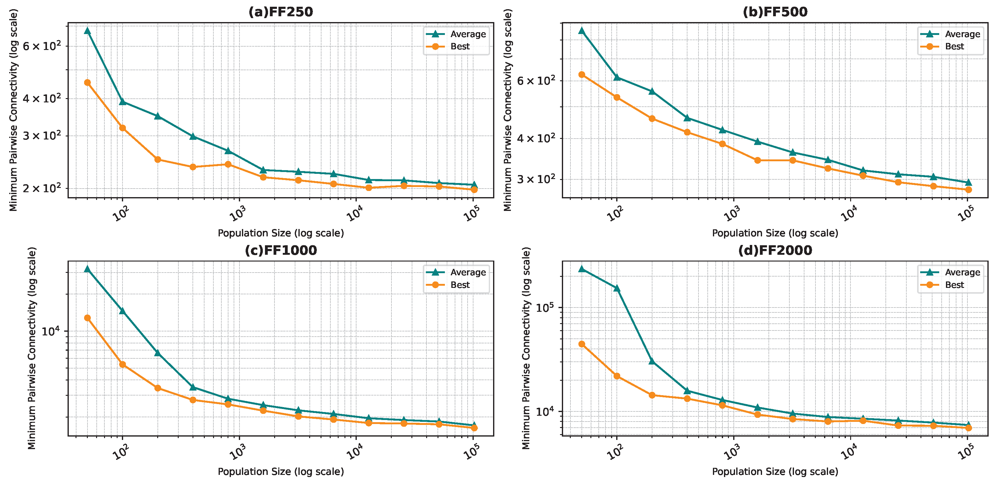
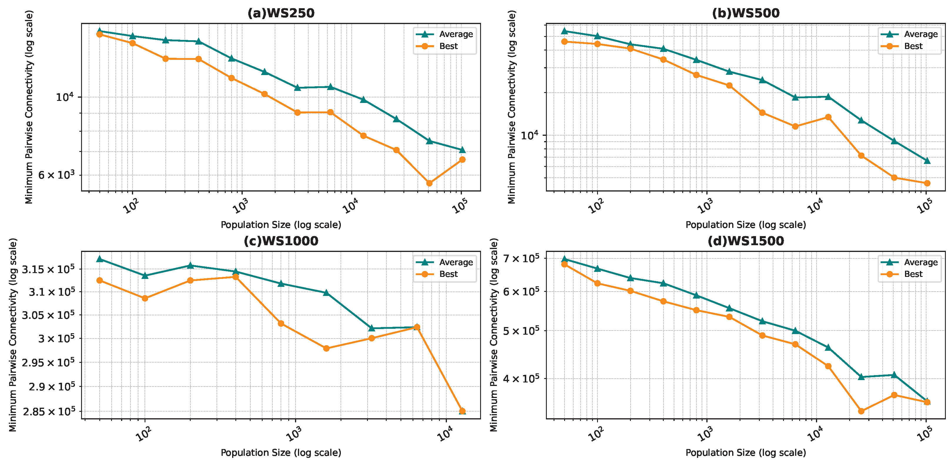
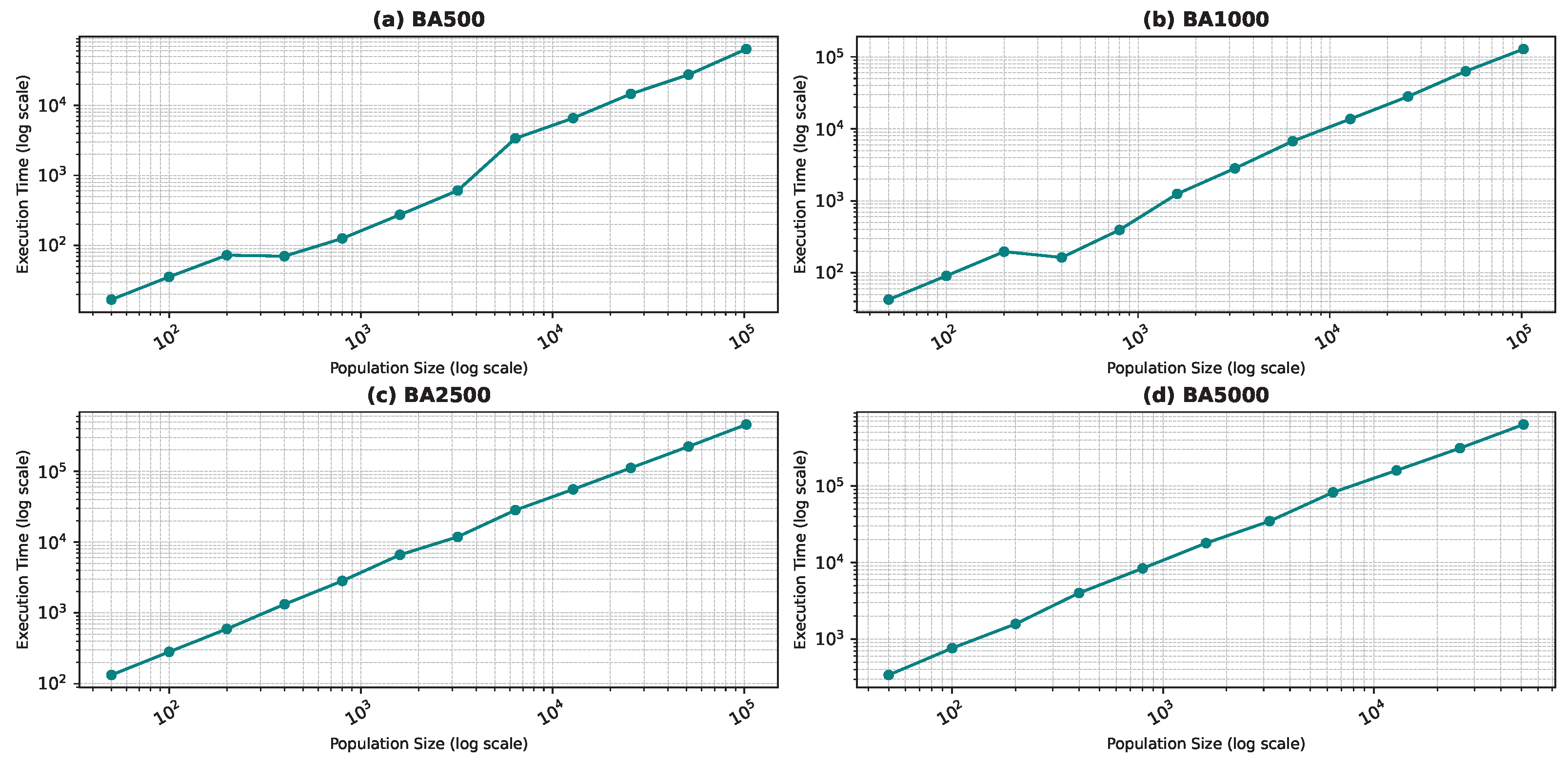
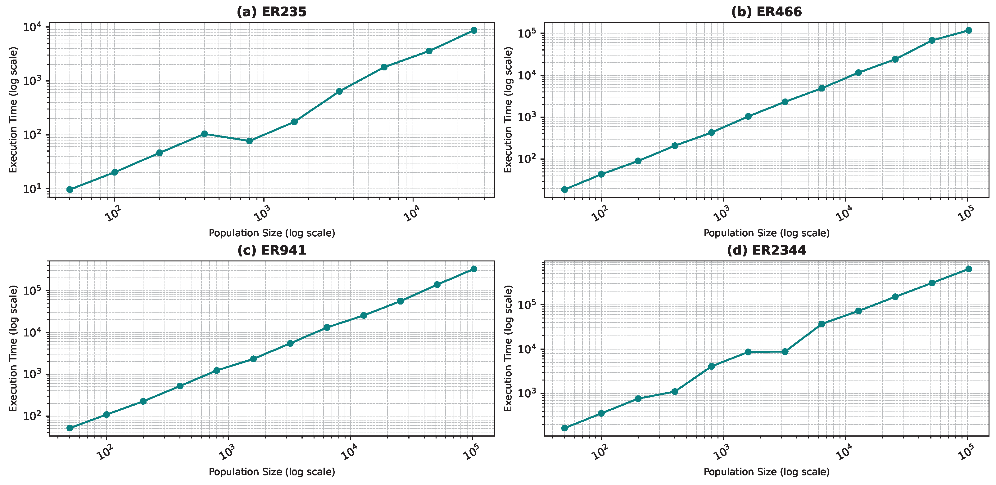
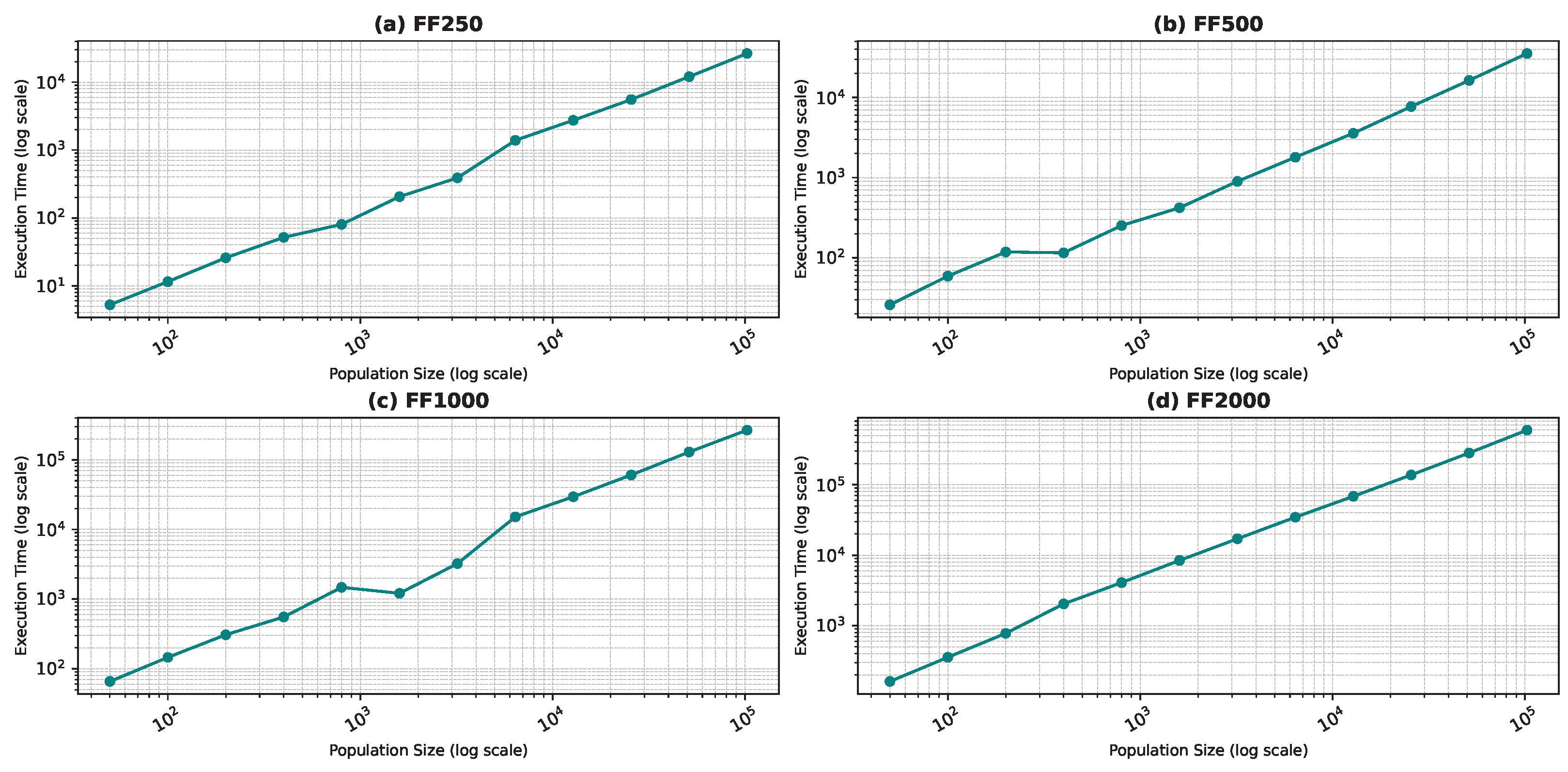
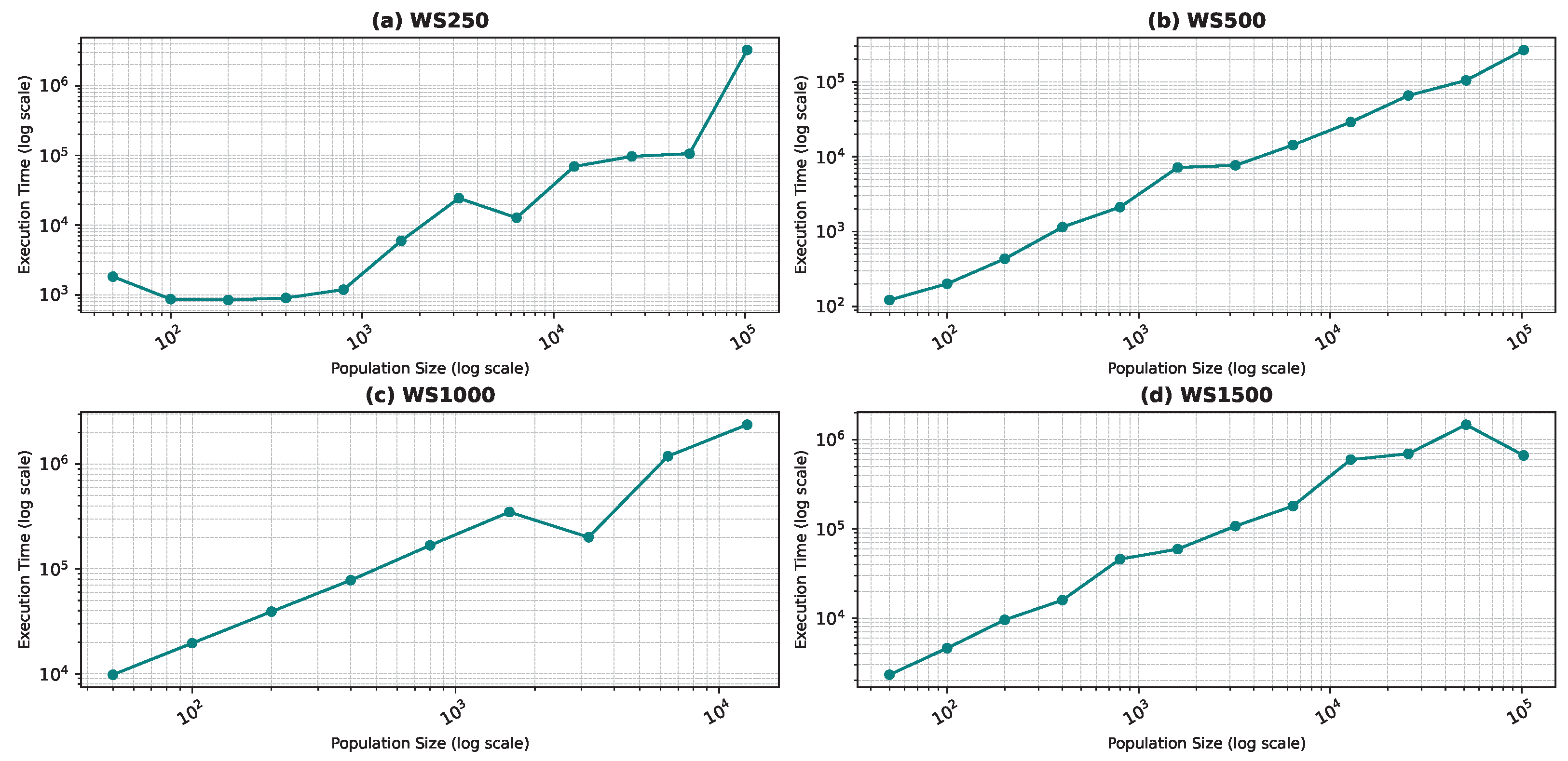
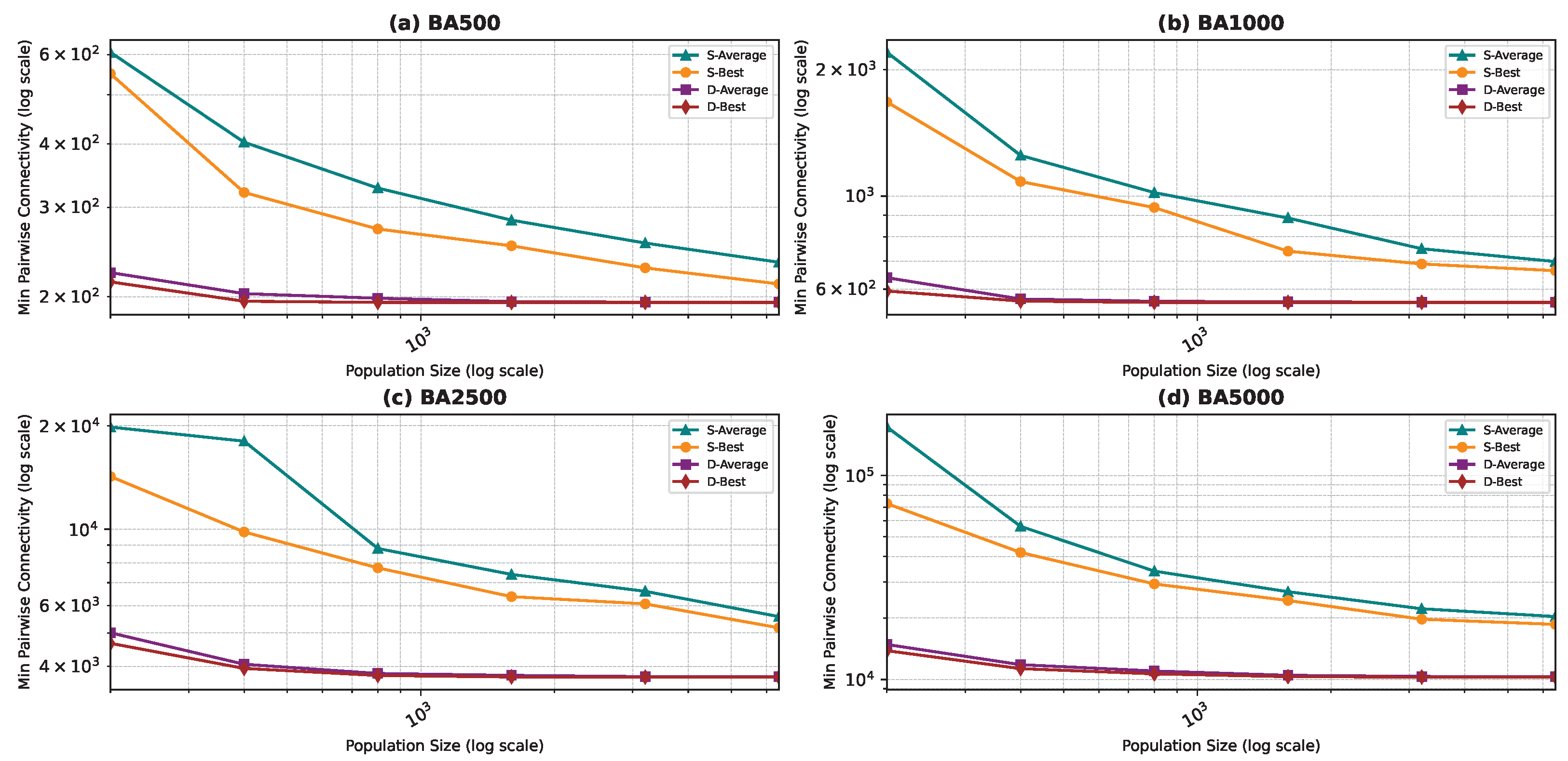
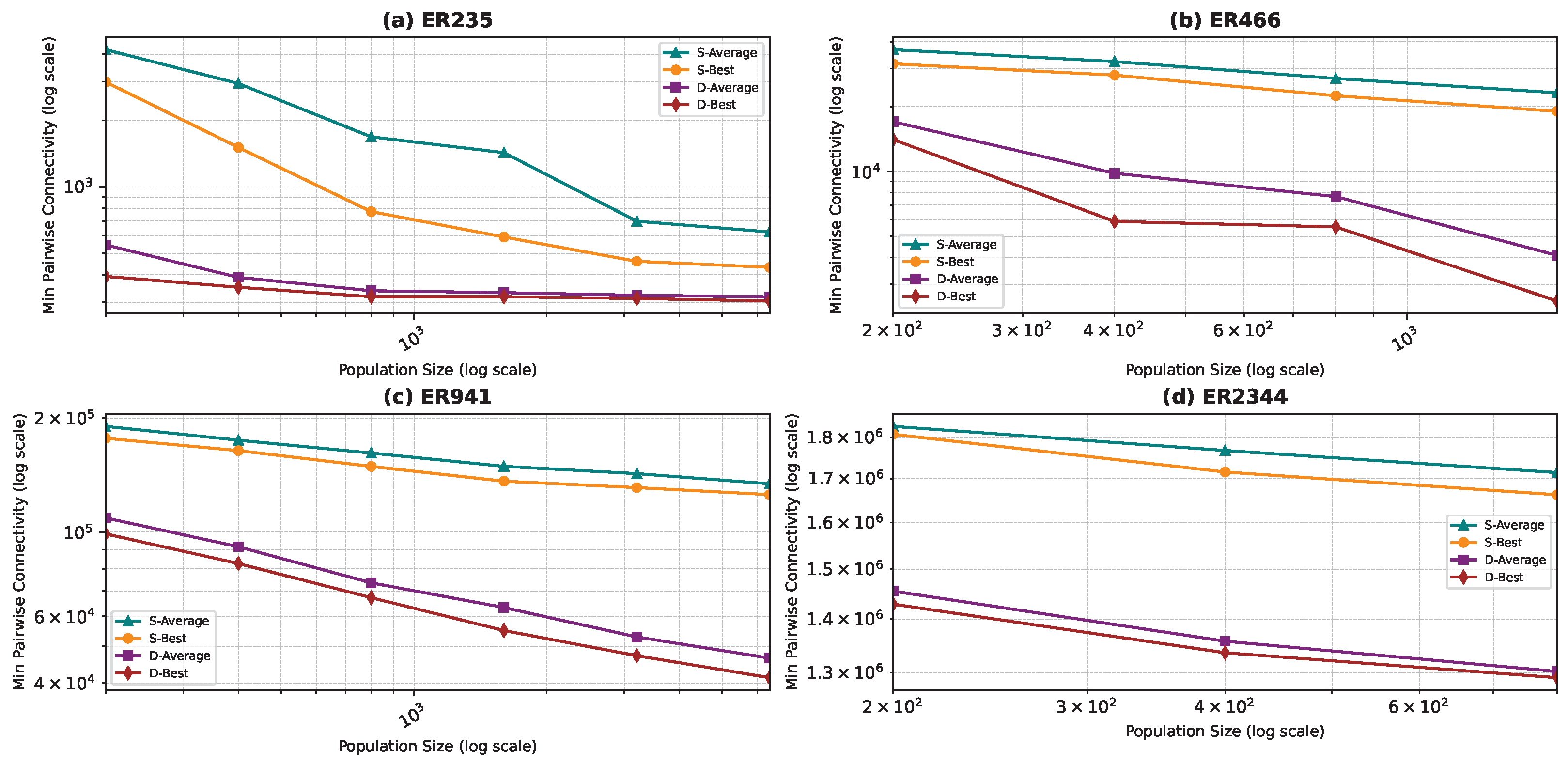
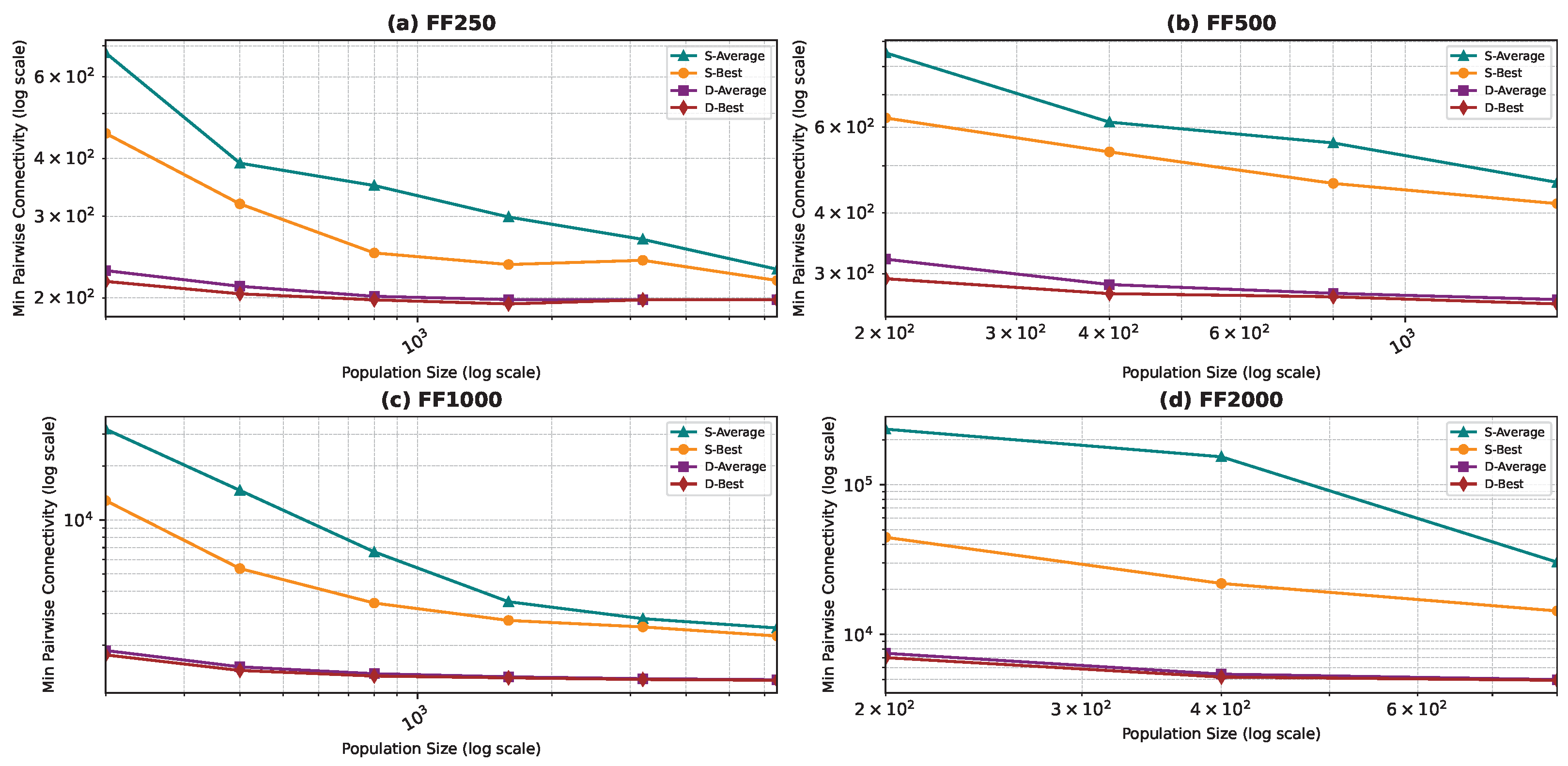
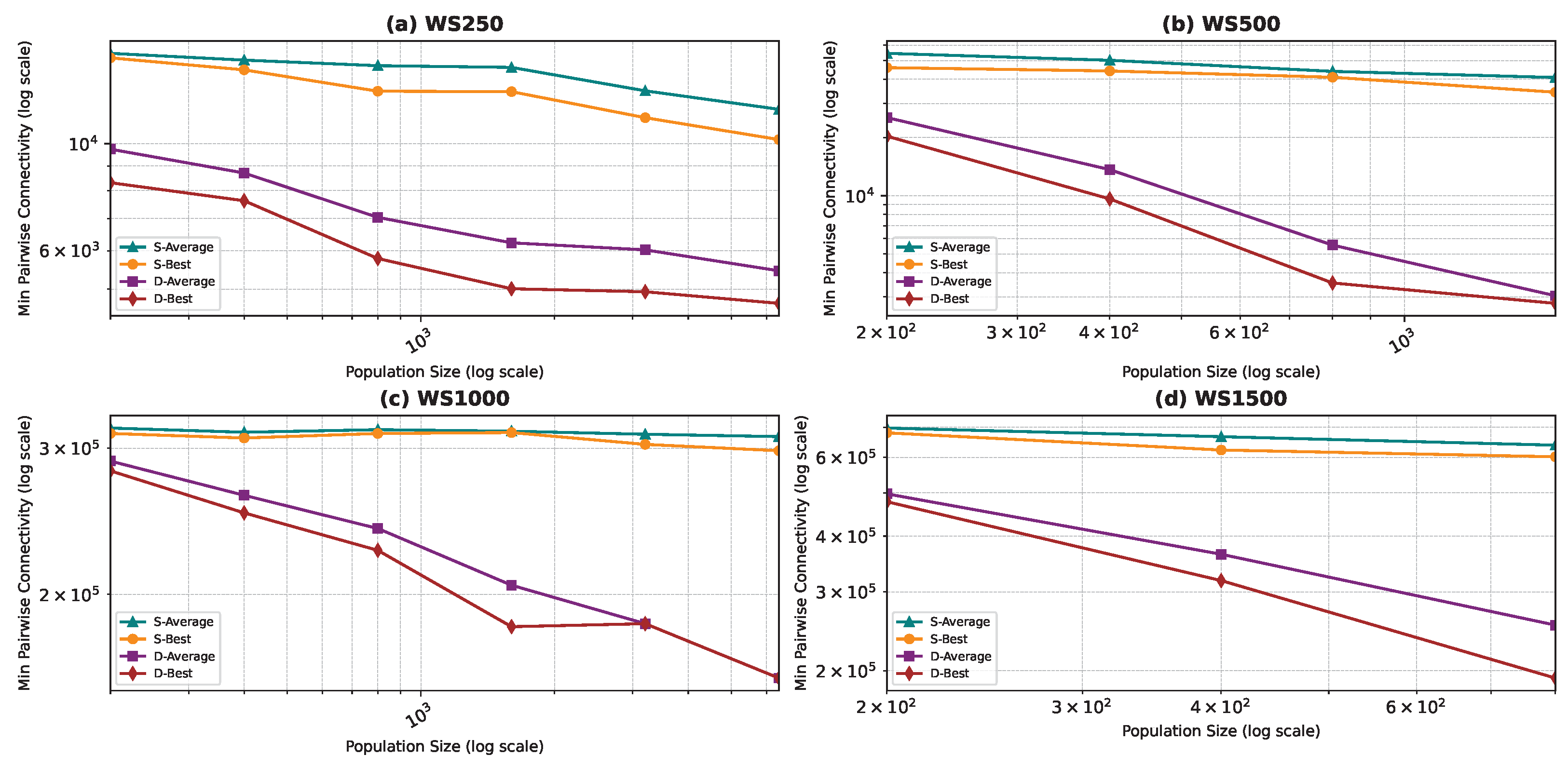
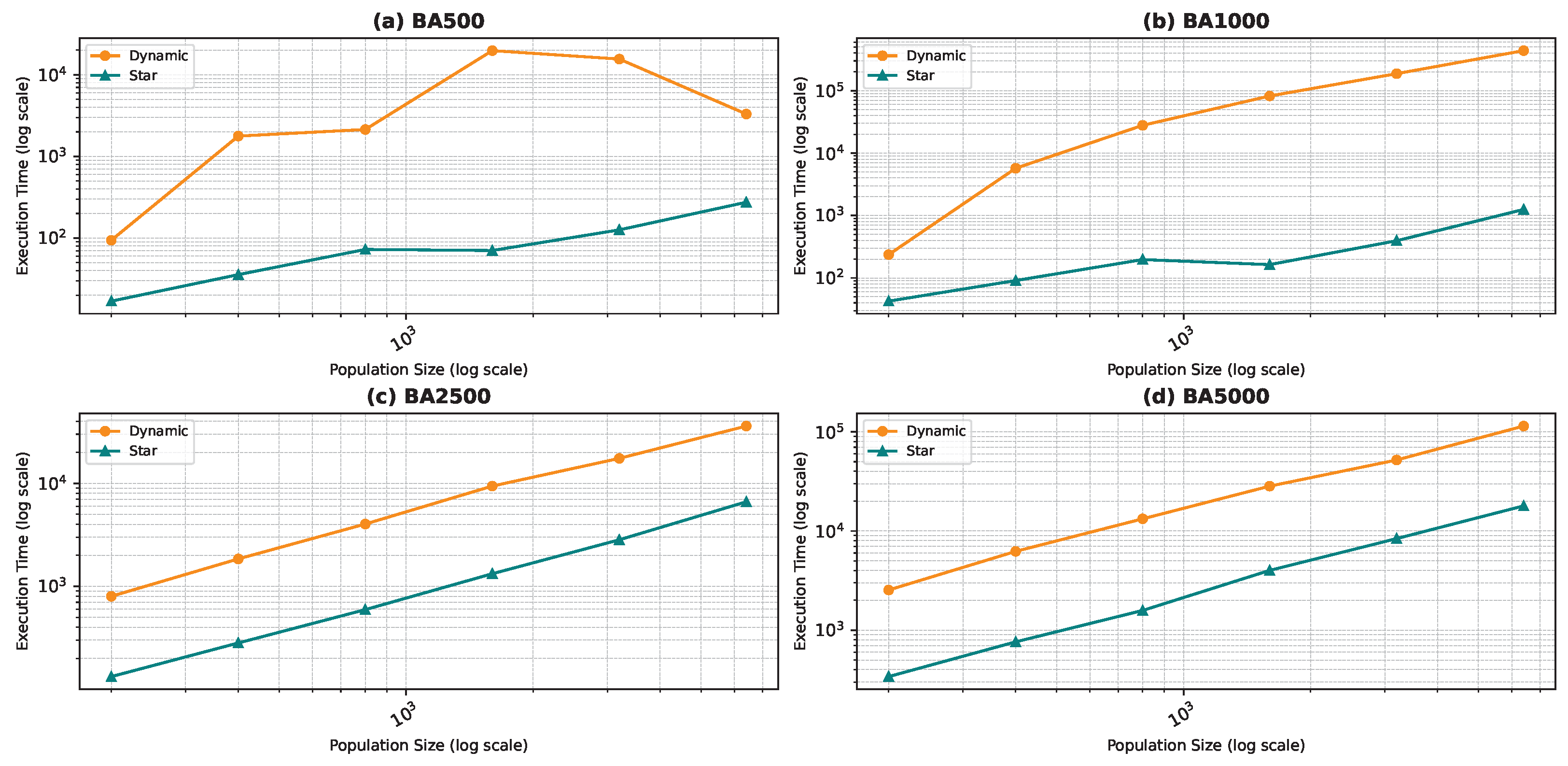
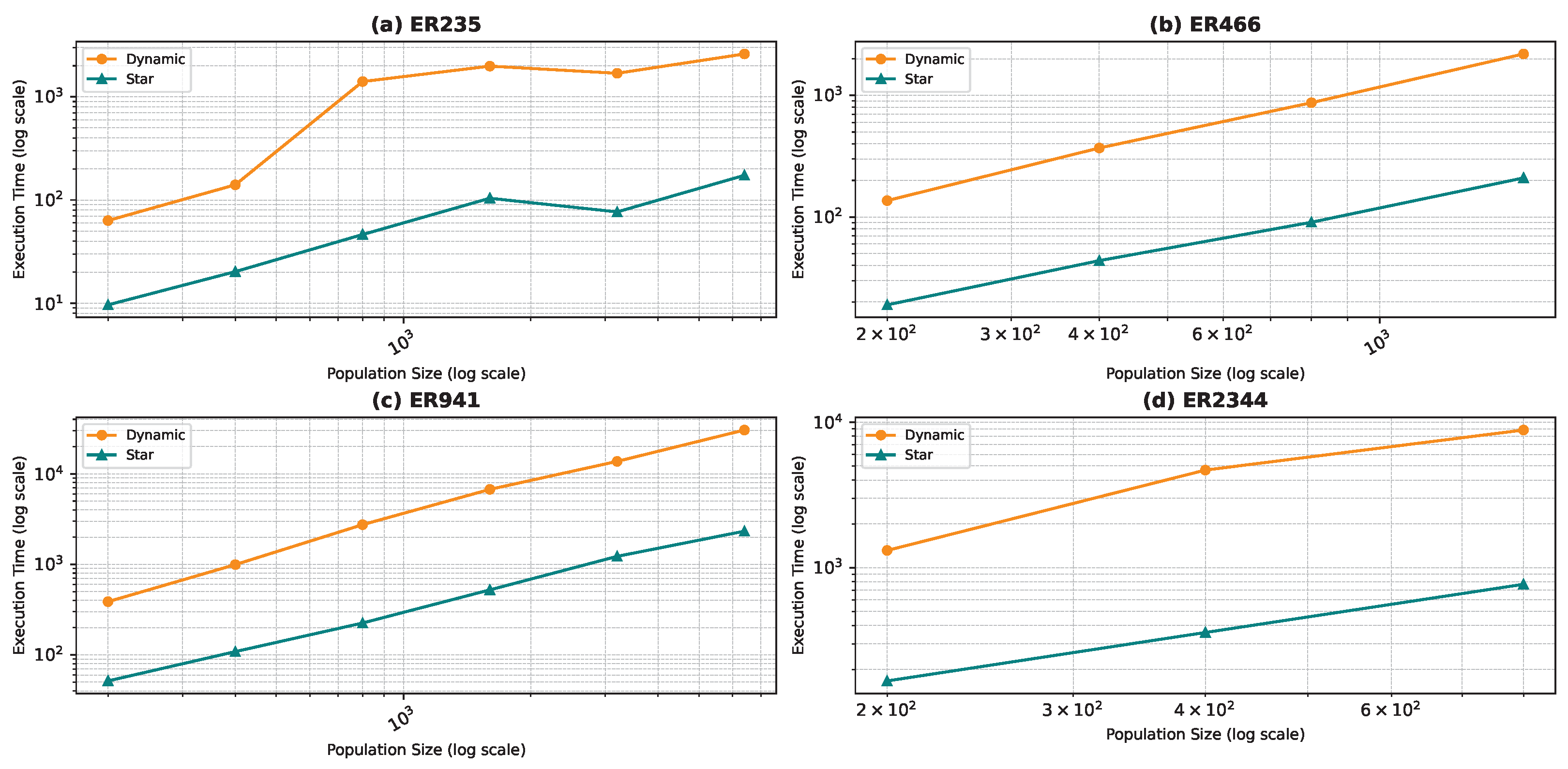
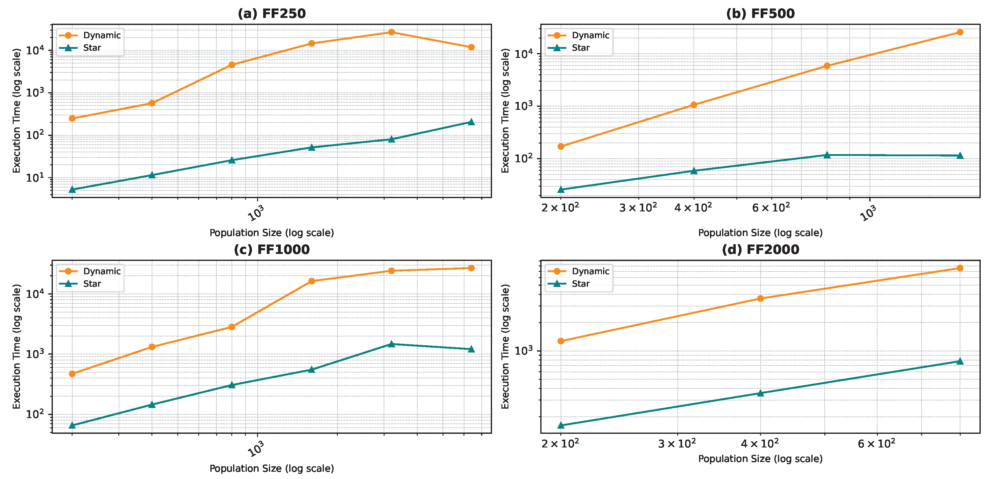

Disclaimer/Publisher’s Note: The statements, opinions and data contained in all publications are solely those of the individual author(s) and contributor(s) and not of MDPI and/or the editor(s). MDPI and/or the editor(s) disclaim responsibility for any injury to people or property resulting from any ideas, methods, instructions or products referred to in the content. |
© 2025 by the authors. Licensee MDPI, Basel, Switzerland. This article is an open access article distributed under the terms and conditions of the Creative Commons Attribution (CC BY) license (https://creativecommons.org/licenses/by/4.0/).