IoT-Based Adaptive Lighting Framework for Optimizing Energy Efficiency and Crop Yield in Indoor Farming

Abstract

Indoor farming presents a sustainable response to urbanization and climate change, yet optimizing light use efficiency (LUE) remains vital for maximizing crop yield and minimizing energy use. This study introduces an IoT-based framework for adaptive light management in controlled environments, using lettuce (Lactuca sativa L.) as a model crop due to its rapid growth and sensitivity to light spectra. The system integrates advanced LED lighting, real-time sensors, and cloud-based analytics to enhance light distribution and automate adjustments based on growth stages. The key findings indicate a 20% increase in energy efficiency and a 15% improvement in lettuce growth compared to traditional static models. Novel metrics—Light Use Efficiency at Growth stage Canopy Level (LUEP) and Lamp Level (LUEL)—were developed to assess system performance comprehensively. Simulations identified optimal growth conditions, including a light intensity of 350–400 µmol/m²/s and photoperiods of 16–17 h/day. Spectral optimization showed that a balanced blue-red light mix benefits vegetative growth, while higher red content supports flowering. The framework’s feedback control ensures rapid (<2 s) and accurate (>97%) adjustments to environmental deviations, maintaining ideal conditions throughout growth stages. Comparative analysis confirms the adaptive system’s superiority over static models in responding to dynamic environmental conditions and improving performance metrics like LUEP and LUEL. Practical recommendations include stage-specific guidelines for light spectrum, intensity, and duration to enhance both energy efficiency and crop productivity. While tailored to lettuce, the modular system design allows for adaptation to a variety of leafy greens and other crops with species-specific calibration. This research demonstrates the potential of IoT-driven adaptive lighting systems to advance precision agriculture in indoor environments, offering scalable, energy-efficient solutions for sustainable food production.

1. Introduction

The global demand for food is projected to increase by 70% by 2050, posing significant challenges due to climate change, shrinking arable land, and resource limitations [1]. Controlled environment agriculture (CEA), particularly indoor and vertical farming, has emerged as a sustainable solution, enabling year-round production, reduced pesticide use, and optimized space efficiency [2,3]. Advances in IoT-enabled sensor networks, LED lighting, and automation have further enhanced precision in regulating microclimatic conditions (light, humidity, temperature, CO₂) [4,5]. Real-world vertical farming deployments such as AeroFarms (Newark, NJ, USA) and Bowery Farming (New York, NY, USA), Futurae Farms (Los Angeles, CA, USA), Farm66 (Tai Po Industrial Estate, Hong Kong), iFarm (Espoo, Finland), and Spread (Fukuroi, Japan) demonstrate the growing reliance on IoT architectures in commercial agriculture, integrating AI, spectral control, and automation to maximize yield and efficiency [6,7,8].

Despite the progress that has been made, light management remains a critical bottleneck in balancing energy efficiency and crop productivity [9]. Most existing systems rely on static lighting protocols (fixed intensity/photoperiod) or generalize photosynthetically active radiation (PAR) without accounting for intra-crop variability or dynamic growth stage adaptation [10]. While recent studies incorporate machine learning and feedback control, many focus on isolated variables (spectrum, photoperiod) rather than holistic, real-time optimization [11,12,13].

To address these gaps, this study introduces an IoT-driven intelligent lighting framework that dynamically adjusts light intensity, spectrum, and photoperiod based on real-time growth stage feedback. Lettuce was selected as the model crop due to its fast growth cycle and sensitivity to light variations, enabling rigorous testing of the IoT framework’s responsiveness and adaptability. While the biological insights are specific to lettuce, the technical architecture is designed with the intention of broader applicability in controlled environment agriculture. By unifying real-time sensor data with adaptive control, this work advances sustainable, data-driven CEA systems beyond current static approaches:

• A growth model for stage-specific lighting adaptation.
• Two novel efficiency metrics: Light Use Efficiency at Growth stage Canopy Level (LUEP) and Lamp-Level Efficiency (LUEL), linking energy input to photosynthetic output.
• A scalable IoT architecture tested on lettuce (Lactuca sativa L.), as a light-sensitive model crop, designed for seamless adaptation to other CEA systems.

2. Literature Review and Research Gaps

Recent advances in IoT-enabled lighting control for indoor farming reveal two dominant disconnected research trajectories: energy optimization and plant response adaptation. Hadj Abdelkader et al. [14] pioneered energy-efficient dynamic lighting but prioritized power savings over photosynthetic efficiency, while Afzali et al. [15] demonstrated scheduled control lacking real-time biomass feedback. Conversely, Jiang et al. [16] incorporated predictive lighting algorithms but omitted growth stage specificity, and Ryu et al. [17] modeled crop dynamics without implementing responsive controls. Ting and Chan [18] enhanced IoT scalability via LoRa networks but did not integrate growth stage level lighting strategies. Collectively, these studies advanced either (1) hardware/energy efficiency or (2) biological growth modeling, but none unified both through real-time, metric driven adaptation, a gap underscored by the absence of LUEP/LUEL-type benchmarks across all works [14,15,16,17,18].

The literature review revealed a critical bifurcation in IoT-enabled lighting systems, with distinct research trajectories for energy optimization versus plant response adaptation. Expanding this analysis to broader agricultural IoT applications, two dominant yet disconnected paradigms emerge: (1) nutrient management systems focusing on soil chemistry and (2) resource optimization platforms targeting water and lighting efficiency, with neither achieving truly integrated control. Recent studies reflect this gap: Lavanya et al. [19] developed a low-cost NPK sensor using colorimetric principles, while Goap et al. [20] integrated machine learning with weather forecasting for irrigation control. However, both systems focus on isolated environmental parameters and lack integration with controls like lighting or feedback loops from growth stage conditions, which limits their adaptability. Moreover, they omit critical metrics such as energy usage or the efficiency of resource application, and neither addresses security vulnerabilities in IoT communications, leaving the systems exposed to potential cyber risks and data breaches.

From a different perspective, Khanna and Kaur [21], in their comprehensive review, emphasize a critical gap in controlled-environment agriculture (CEA): light use efficiency (LUE). While soil and water systems are relatively mature, light optimization, especially real-time, plant-stage responsive control, remains underexplored. Existing IoT implementations such as Bodunde et al.’s mobile robots [22] or Foughali et al.’s disease detection system [23] show promise but fail to integrate plant-level feedback for adaptive decision-making. Bodunde’s system lacks control over lighting or nutrient coordination, and Foughali’s cloud-based architecture introduces high latency and offers no real-time responsiveness. Additionally, both systems fail to account for energy performance or data security, which are increasingly important in modern, autonomous CEA systems.

A thorough analysis of the existing IoT-enabled indoor farming systems demonstrates distinct technological approaches: precision nutrient management, environmental parameter control, energy optimization, and advanced sensing methodologies. The following analysis critically examines recent studies in each domain:

• Lavanya et al. [19]:

Focus: Low-cost NPK (nitrogen, phosphorus, potassium) monitoring in soil.

Method: Colorimetric sensors with CoAP/UDP protocols for real-time nutrient detection.

Strength: Affordable hardware (<USD 50) and 85% accuracy in nutrient measurements.

Limitation: No integration with lighting or irrigation controls; standalone soil analysis.

• Goap et al. [20]:

Focus: Irrigation optimization using machine learning (ML).

Method: ML models trained on weather forecasts and soil moisture data (HTTP-based IoT).

Strength: Reduced water usage by 30% compared to timer-based systems.

Limitation: Ignores light energy trade-offs; no multi-parameter coordination.

• Khanna and Kaur [21]:

Focus: Comprehensive survey identifying gaps in controlled-environment agriculture (CEA), especially light use efficiency (LUE).

Method: Literature review analyzing IoT applications in precision agriculture.

Strength: Highlights critical gap in real-time, plant-stage light management.

Limitation: Does not propose a practical system; identifies issues but lacks experimental validation.

• Bodunde et al. [22]:

Focus: Mobile robotic irrigation for precision water delivery.

Method: ZigBee-controlled robots mapping soil moisture variability.

Strength: Dynamic water allocation (20% yield improvement in uneven fields).

Limitation: No light or nutrient coordination; limited to greenhouse-scale deployments.

• Foughali et al. [23]:

Focus: Early disease detection in leafy greens.

Method: ZigBee/Cloud-IoT hybrid system with a decision support system (DSS).

Strength: Real-time disease alerts (90% detection accuracy).

Limitation: No adaptation to growth stages; high latency (~minutes).

• Zhang et al. [3]:

Focus: Light intensity optimization for lettuce growth.

Method: Fixed PAR (photosynthetically active radiation) thresholds (350–400 µmol/m²/s).

Strength: Demonstrated 12% faster growth at optimized intensity.

Limitation: Static spectra; no real-time or canopy-level adjustments.

• Benyezza et al. [24]:

Focus: Smart irrigation zoning.

Method: Wireless sensor network (WSN) + Fuzzy Logic Controller (FLC) integrated into IoT architecture.

Strength: Efficient water and energy usage with zone-specific control.

Limitation: No adaptation to light or disease dynamics.

• Raghuvanshi et al. [25]:

Focus: Security in smart agriculture.

Method: SVM and Random Forest-based Intrusion Detection System (IDS) for irrigation control.

Strength: A total of 98% detection accuracy in identifying cyber threats.

Limitation: Focused on network-level security, not sensing or plant-level feedback.

• Chataut et al. [26]:

Focus: Comprehensive IoT meta-analysis.

Method: Literature survey of agricultural IoT technologies.

Strength: Identifies security, energy, and integration as key bottlenecks.

Limitation: No original system or deployment.

• Javaid et al. [27]:

Focus: Agriculture 4.0 integration.

Method: Combining AI, IoT, robotics, and blockchain.

Strength: System-wide digital transformation across multiple domains.

Limitation: Conceptual framework without specific energy metrics or sensor feedback.

• Seesaard et al. [28]:

Focus: Gas sensors and electronic noses (E-noses) for full agricultural cycle.

Method: Review of gas sensor evolution and E-nose applications in cultivation, harvesting, and storage.

Strength: Covers a wide range of sensing modalities including MOS and nanomaterial-based sensors.

Limitation: Primarily a review; lacks deployment-level metrics or integration into IoT automation.

Table 1. Comparative analysis of IoT systems in smart agriculture.

Study	Primary Focus	Methodology	Multi-Parameter Control	Real-Time Adaptation	Security/IDPS	Energy Metrics	Latency	Key Innovation
Lavanya et al. [19]	Soil NPK monitoring	Colorimetric NPK sensor + CoAP/UDP	Limited to soil nutrients only; no coordination with other environmental factors	Lacks dynamic response; measurements are taken and sent without adaptive action	No intrusion detection or security protocols implemented	No measurement or optimization of energy usage	Approximately 300 ms	Affordable and compact NPK sensor integration
Goap et al. [20]	Irrigation optimization	ML-based irrigation using weather and soil data	Focused only on soil moisture and weather; does not integrate light or nutrient feedback	No real-time growth stage sensing; ML decisions are pre-trained and not plant-responsive	No discussion or handling of cybersecurity risks	Does not track energy use in pumping or communication	Approximately 300 ms	Predictive irrigation through ML modeling
Khanna and Kaur [21]	Survey of IoT gaps in precision agriculture and CEA	Literature review of top cited IoT studies in agriculture	Identifies lack of integration across systems	Highlights missing dynamic responsiveness	Notes security concerns but lacks implementation	Emphasizes absence of plant-level energy use metrics	Recognizes delays in feedback systems	Maps critical research gaps like LUE, energy waste, and lack of closed loop control
Bodunde et al. [22]	Mobile irrigation	ZigBee communication with mobile robot	Focuses solely on soil moisture distribution; no coordination with light or nutrient control	Partially adaptive to soil moisture maps but not fully autonomous or continuous	No security measures for robot control or data streams	No mention of power efficiency of mobile units	Around 100 ms	Water precision via robotic mobility
Foughali et al. [23]	Disease prevention	ZigBee-based sensing + cloud DSS	Addresses disease and climate but lacks integration with lighting, irrigation, or nutrients	Not responsive to growth stage conditions in real time; latency in cloud processing	No built-in protection against data interception or tampering	Energy consumption not assessed, despite continuous monitoring	Several minutes due to cloud processing	Early detection of growth stage disease via DSS
Zhang et al. [3]	Light intensity optimization	Static light control using fixed PAR values	Optimizes light but does not consider nutrient, water, or temperature interactions	Uses fixed values; no growth stage feedback or stage-based adjustment	No protection mechanisms for network or device security	Energy use implied but not analyzed in light energy terms	Not specified	Demonstrated improved growth from PAR tuning
Benyezza et al. [24]	Zoning irrigation	Fuzzy logic control with wireless sensors	Coordinates soil moisture and temperature in specific zones but excludes light or nutrient metrics	Adaptable zoning improves local responses but lacks real-time growth stage sensing	No security or encryption techniques used in WSN	Improves water efficiency, but no broader energy assessment	Less than 1 s	Intelligent irrigation zoning through FLC
Raghuvanshi et al. [25]	Cybersecurity in agriculture	Machine learning-based IDS for smart irrigation	Focused on network-layer threats; does not manage any growth stage or environmental parameters	No feedback from plants or sensors; strictly a cyber-layer solution	High-accuracy intrusion detection using SVM and Random Forest	Energy use of the IDS or system not considered	Not applicable	Strong threat detection for agricultural IoT
Chataut et al. [26]	Literature survey	Review of agricultural IoT trends and tools	Identifies challenges across multiple domains but lacks specific system implementation	Synthesizes past work rather than proposing adaptive strategies	Points out security gaps but does not propose or test solutions	Recognizes need for energy efficiency but lacks quantitative data	Not applicable	Comprehensive identification of research bottlenecks
Javaid et al. [27]	Agriculture 4.0 integration	Conceptual model combining AI, IoT, robotics, and blockchain	Promotes system-wide synergy but remains theoretical without deployment details	Predictive in concept, but no direct sensor–actuator implementation shown	Discusses blockchain potential but lacks direct experimentation	Energy efficiency assumed in abstract terms, not measured	Not applicable	Conceptual integration of next-gen agri-technologies
Seesaard et al. [28]	Gas sensing in agriculture	Review of gas sensor and E-nose technologies	Broad in sensor types but not integrated with environmental controls or decision systems	Provides sensing options but lacks discussion on automation or feedback loops	Focuses on sensor function; no attention to data privacy or network safety	Technical discussion of sensors only; no analysis of power use in context	Not applicable	Extensive catalog of E-nose and gas sensor evolution
Our System	LUE-based optimization	Logistic growth model + real-time sensor–actuator feedback	Integrates light, soil moisture, and canopy health for closed-loop control	Dynamically adjusts spectrum and intensity based on growth stage needs	Currently lacks built-in security layer; potential for future integration	Tracks energy efficiency using LUEP and LUEL	Under 2 s end-to-end	Real-time optimization of light use for biomass gain

below highlights the strengths and critical gaps of existing IoT-enabled agriculture studies, emphasizing how our system advances prior work by addressing light use efficiency, energy metrics, and real-time growth stage adaptation, features which are largely missing in the current research.

3. Materials and Methods

3.1. System Architecture and Hardware Setup

The IoT prototype for growing plants indoors is a compact and insulated setup designed for experimental purposes. The structure is composed of clear plexiglass panels forming the walls, allowing visibility inside the enclosure, with the top and bottom parts made of wood, providing a sturdy base and support for the overall structure. Inside the enclosure, we have a Raspberry Pi board for control and data processing, an Arduino with relay modules for managing electronic connections and control mechanisms, a breadboard for prototyping circuits, and a cooling fan to regulate internal temperature. Various wires and connections link the components together. We designed the enclosure to be insulated in order to maintain a controlled environment for testing various light configurations, making it suitable for IoT integration, automation, and indoor climate management, as illustrated in Figure 1 below. Other tests of light configurations were performed through simulations. The experiment was conducted from May to December 2024, with iterative testing and system optimization. The final 4-week evaluation phase (December 2024) provided the definitive dataset used for the analysis, ensuring stable IoT performance and consistent cultivation conditions. Data collection spanned this entire period, but only the optimized results from the conclusive phase were included in the reported findings.

A breadboard is used for circuit prototyping, and a cooling fan is included to regulate the internal temperature, as shown in Figure 1a. The lighting system, shown in Figure 1b, includes strategically placed LED fixtures to ensure uniform light distribution across the chamber. Environmental monitoring capabilities are enhanced with an IoT-based CO₂ sensing module, which features a Wemos D1 microcontroller and a CO₂ sensor mounted on a prototype board for real-time gas concentration tracking, as shown in Figure 1c. Additionally, temperature and humidity are measured using a DHT22 sensor, with data acquisition handled by another Wemos D1 board; a pull-up resistor ensures signal reliability in this sensing module, as shown in Figure 1d.

The technical specifications of the LED lighting system are summarized in

Table 2. LED physical properties.

Property	Details
LED Model	Programmable full-spectrum LED panels
Brightness (PAR)	150–400 µmol/m2/s
Power	25 W per LED panel
Temperature	Operating range: 22–25 °C
Control	Raspberry Pi + Arduino relay modules
Spectral Ratios	Seedling: High blue (0.3:0.7:0.0)
	Vegetative: Balanced blue-red (0.2:0.7:0.1)
	Flowering: High red (0.1:0.8:0.1)

below:

3.2. Wired Sensor Network

Figure 2a in Figure 2 illustrates the Wi-Fi-enabled integration of the light sensor, Azure IoT Hub, and Raspberry Pi to monitor and control LED lighting based on real-time data for optimal growth stage growth. In this indoor farming setup, the light sensor continuously measures intensity and sends data over Wi-Fi to the Raspberry Pi, which publishes them to Azure IoT Hub. The Azure App then evaluates the light levels and sends MQTT commands back to the Raspberry Pi to adjust the LED system. If the intensity is too low, the LEDs are brightened, and if it is too high, they are dimmed; otherwise, the lighting is maintained at an optimal level.

Figure 2b in Figure 2 illustrates the IoT-based lighting control architecture, where the light sensor relays intensity data to a Raspberry Pi MQTT broker. The broker publishes these measurements to Azure IoT Hub over the specified Ethernet, allowing the cloud to process and store the data. MQTT commands are then returned to the actuator, which executes the required lighting adjustments.

3.3. Wireless Sensor Network

Figure 3a below shows that the Wemos D1-R3 microcontroller constitutes the Wi-Fi-based sensor and actuator unit. It digitizes the measured input data and sends them to the cloud application. The microcontroller then controls the actuator output based on the received data.

Figure 3b below shows that one Wemos D1-R3 microcontroller serves as the Wi-Fi-based sensor and the other as the actuator unit. The sensor digitizes the input data and sends them to the actuator unit, which then evaluates the received data to control the output.

3.4. Analysis of Time Responsiveness in IoT Communication

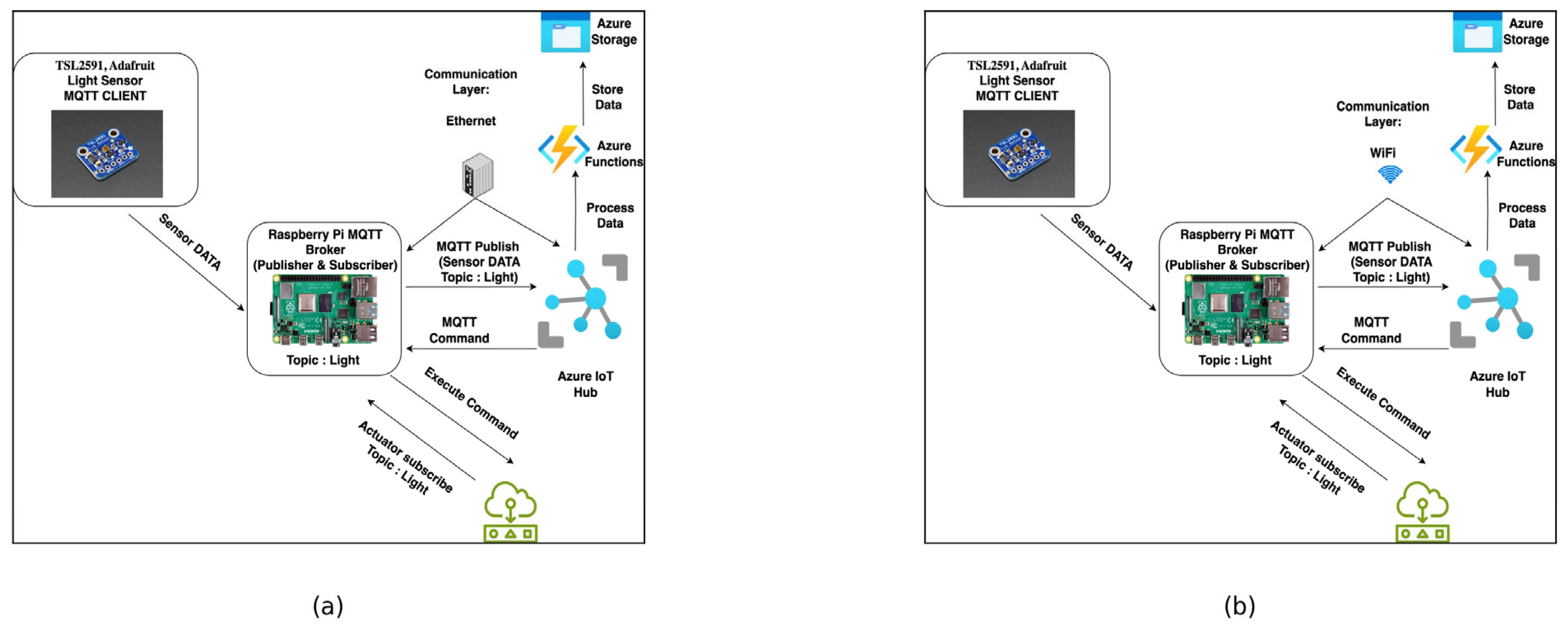
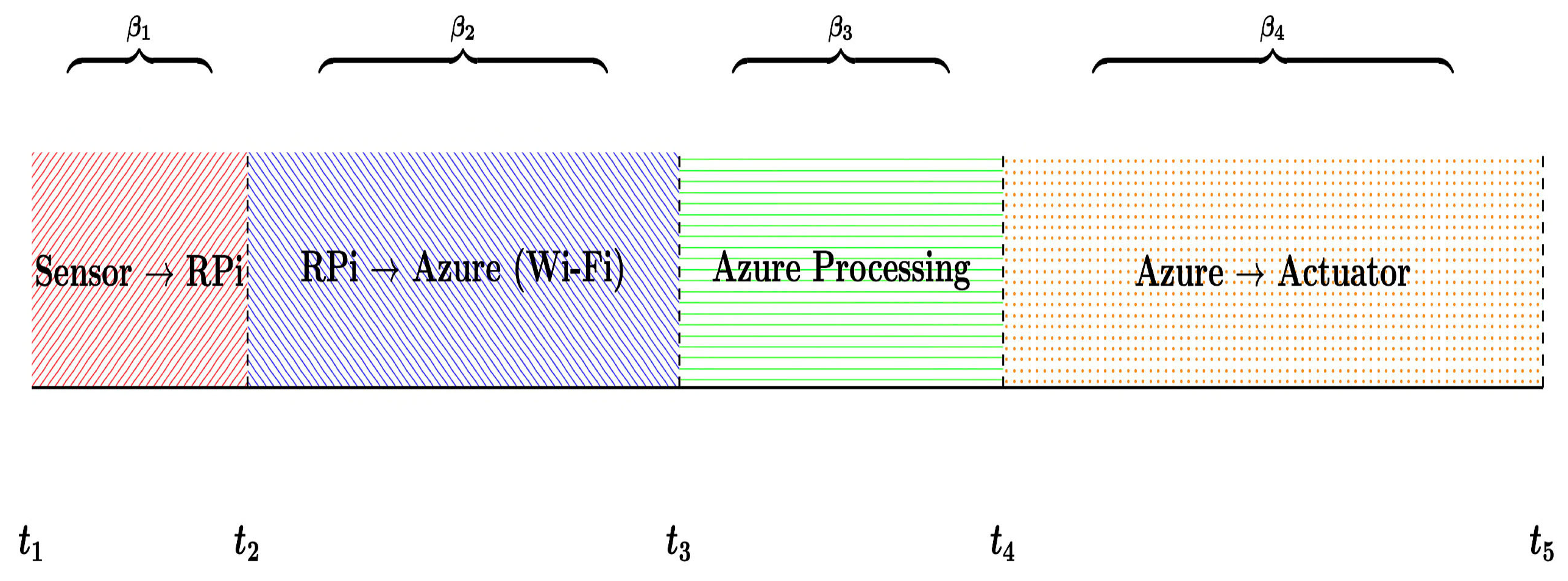
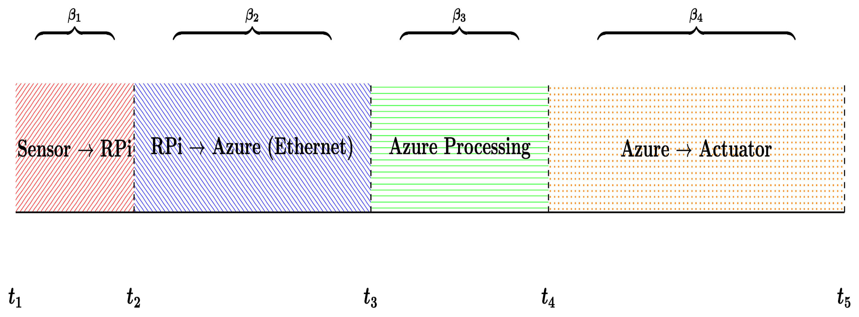
3.4.1. Time Responsiveness in Wi-Fi vs. Ethernet in MQTT-Based IoT System

To compute the end-to-end responsiveness of our MQTT-based IoT system, we model the overall delay, Ψ, as the sum of the delays in each segment of the communication path, as shown in Equation (1):

$$\Psi ={\mathsf{\beta }}_1+{\mathsf{\beta }}_2+{\mathsf{\beta }}_3+{\mathsf{\beta }}_4$$

(1)

where

${\mathsf{\beta }}_1$ represents the delay for the sensor node to measure and prepare the data;

${\mathsf{\beta }}_2$ is the communication delay from the sensor (or intermediate gateway) to the cloud, which we further define as in Equation (2):

$${\mathsf{\beta }}_2={\displaystyle \frac{\mathbf{S}}{\mathbf{B}}}+{\mathbf{T}}_{\mathbf{p}}$$

(2)

where S is the size of the message in bits, B is the effective bandwidth (differing between Wi-Fi and Ethernet), and ${\mathbf{T}}_{\mathbf{p}}$ captures additional propagation or processing overhead.

${\mathsf{\beta }}_3$ accounts for the processing delay within the cloud (including any function execution and data storage);

${\mathsf{\beta }}_4$ is the delay for the command to travel back from the cloud to the actuator.

For instance, when comparing Wi-Fi versus Ethernet, we have Equations (3) and (4), respectively:

$${\mathsf{\beta }}_2^{\mathbf{W}\mathbf{i}\mathbf{F}\mathbf{i}}={\displaystyle \frac{\mathbf{S}}{{\mathbf{B}}_{\mathbf{W}\mathbf{i}\mathbf{F}\mathbf{i}}}}+{\mathbf{T}}_{\mathbf{p}}^{\mathbf{W}\mathbf{i}\mathbf{F}\mathbf{i}}$$

(3)

$${\mathsf{\beta }}_2^{\mathbf{E}\mathbf{t}\mathbf{h}\mathbf{e}\mathbf{r}\mathbf{n}\mathbf{e}\mathbf{t}}={\displaystyle \frac{\mathbf{S}}{{\mathbf{B}}_{\mathbf{E}\mathbf{t}\mathbf{h}\mathbf{e}\mathbf{r}\mathbf{n}\mathbf{e}\mathbf{t}}}}+{\mathbf{T}}_{\mathbf{p}}^{\mathbf{E}\mathbf{t}\mathbf{h}\mathbf{e}\mathbf{r}\mathbf{n}\mathbf{e}\mathbf{t}}$$

(4)

Figure 4 and Figure 5 illustrate the four segments of the end-to-end delay Ψ from Equation (1), showing how each phase (${\mathbf{\beta }}_1$, ${\mathbf{\beta }}_2$, ${\mathbf{\beta }}_3$, ${\mathbf{\beta }}_4$) contributes to overall responsiveness. The red section corresponds to sensor node preparation (${\mathbf{\beta }}_1$), blue indicates communication between the Raspberry Pi and the cloud (${\mathbf{\beta }}_2$), green represents cloud processing (${\mathbf{\beta }}_3$), and yellow covers the return path from the cloud to the actuator (${\mathbf{\beta }}_4$). In the Wi-Fi scenario (Figure 2b), the communication delay (${\mathbf{\beta }}_2$) is typically larger due to lower bandwidth and higher overhead, whereas in the Ethernet scenario (Figure 2a), this segment is reduced, reflecting the faster, more stable wired connection.

Furthermore, if retransmissions are required due to packet loss, the effective delay increases by a factor of 1/${\mathbf{P}}_{\mathbf{s}\mathbf{u}\mathbf{c}\mathbf{c}\mathbf{e}\mathbf{s}\mathbf{s}}$, where ${\mathbf{P}}_{\mathbf{s}\mathbf{u}\mathbf{c}\mathbf{c}\mathbf{e}\mathbf{s}\mathbf{s}}$ is the probability of a successful transmission, as shown in Equation (5):

$${\mathsf{\Psi }}_{\mathbf{e}\mathbf{f}\mathbf{f}}=\Psi \times {\displaystyle \frac{1}{{\mathbf{P}}_{\mathbf{s}\mathbf{u}\mathbf{c}\mathbf{c}\mathbf{e}\mathbf{s}\mathbf{s}}}}$$

(5)

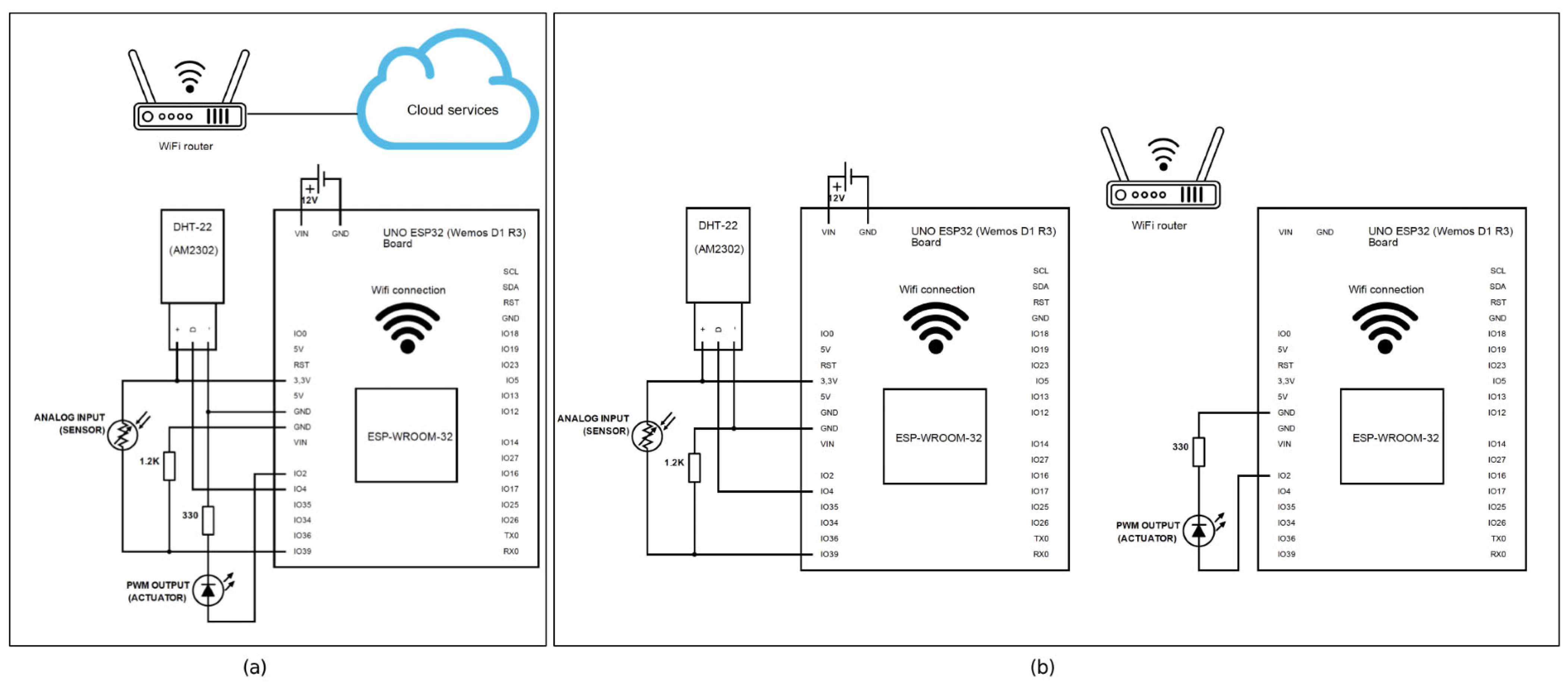
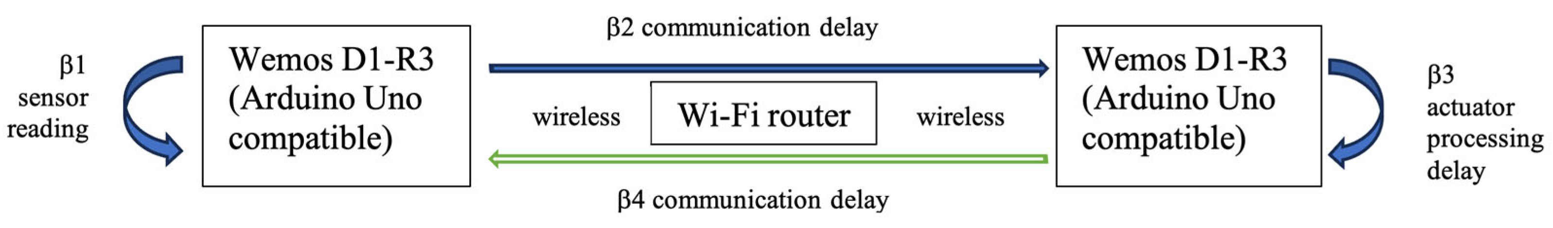
3.4.2. Time Responsiveness in Point-to-Point vs. Cloud in HTTP-Based IoT System

Figure 6 shows a setup where the Arduino-based microcontroller reads physical sensor data with a delay β1. The microcontroller is connected to the router via Wi-Fi, and from there the connection is wired to the cloud application with a communication delay. β2. β3 processing time is used by the cloud application to evaluate the sensor data, and β4 communication delay is used to return the control data to the microcontroller. The microcontroller controls the actuator control with a delay β5.

To compute the end-to-end responsiveness for Wi-Fi-based sensor to cloud communication using the HTTP protocol, we model the overall delay, Ψ, as the sum of the delays in each segment of the communication path, as modeled in Figure 6 and shown in Equation (6):

$$\Psi ={\mathsf{\beta }}_1+{\mathsf{\beta }}_2+{\mathsf{\beta }}_3+{\mathsf{\beta }}_4+{\mathsf{\beta }}_5$$

(6)

The measurement was performed within the microcontroller unit, where we measured the various latency times, while the execution time in the cloud was returned packaged in the response. The data arrived in a JSON structure in response to the HTTP request. Based on the received data, the PWM duty cycle of the output can be set, which, when connected to the input of the LED light source, determines the intensity of the grow light. The total communication delay consists of 5 elements.

Figure 7 shows another setup where one Arduino-based microcontroller reads physical sensor data with a delay β1 and then connects to the other microcontroller via Wi-Fi with a delay β2. The actuator control takes β3 time. The communication is acknowledged with a delay β4.

The series of measurements consisted of 500 queries. To compute the end-to-end responsiveness for Wi-Fi-based sensor point-to-point communication using the HTTP protocol, we model the overall delay, Ψ, as the sum of the delays in each segment of the communication path, as modeled in Figure 7 and shown in Equation (7):

$$\Psi ={\mathsf{\beta }}_1+({\mathsf{\beta }}_2+{\mathsf{\beta }}_4) /2+{\mathsf{\beta }}_3$$

(7)

The measurement was performed within the sensor microcontroller unit, where we were able to measure the different latency times. The latency time indicated by the green arrow is not included in the total processing time; it was only included for accurate measurement purposes. The actuator unit’s latency time was received in the response. The response to the HTTP request returned the data in JSON format. The received data are evaluated by the actuator unit, which sets the PWM duty cycle for the output, determining the light intensity of the grow light connected to the LED light source input. The total communication latency consists of 3 elements.

3.4.3. Technology Trade-Offs in IoT Responsiveness

In evaluating the time responsiveness of our MQTT-based IoT system, it is critical to contextualize ${\mathbf{\beta }}_2$ (communication delay) within broader network characteristics. Beyond latency, which directly affects the effective bandwidth, scalability, energy consumption, and range of communication technologies also shape system responsiveness and performance. Ethernet offers low latency and high bandwidth but limited range and scalability, making it ideal for static, high-throughput scenarios. Wi-Fi provides moderate latency and bandwidth, with better mobility support but higher energy consumption and interference susceptibility. In contrast, technologies like LoRaWAN prioritize energy efficiency and extended range, sacrificing latency and throughput. NB-IoT balances energy and range with better reliability under dense deployments.

3.5. Lighting Configuration and Feedback Control

We propose a feedback control system for optimizing growth stage growth by dynamically adjusting light intensity in real time. This system bridges the gap between static growth models and practical applications in smart agriculture by introducing a data-driven decision-making framework.

Previous models [29] focused primarily on static simulations of growth as a function of light intensity and spectrum. Our model advances this by integrating real-time feedback control with a dynamic threshold adjustment mechanism. Unlike traditional approaches that rely on fixed thresholds, our system dynamically adjusts (${\mathbf{T}}_{\mathbf{l}\mathbf{o}\mathbf{w}},{\mathbf{T}}_{\mathbf{h}\mathbf{i}\mathbf{g}\mathbf{h}}$) based on variables such as ambient light and growth stages, ensuring more responsive environmental adaptation.

This work represents a critical progression beyond our previous research. In [30], we addressed water level monitoring in precision agriculture using fixed threshold logic; however, it lacked intelligent control or integration with lighting or other environmental factors. The system in that study could only detect critical water levels, generating binary alarms, whereas the current system interprets multi-modal sensor data for continuous control. In [31], we explored phenotyping and image-based growth stage growth monitoring, but the insights were used solely for analysis, not for real-time decision-making or actuation. In contrast, our current system incorporates real-time image analysis into an active feedback loop that adjusts lighting conditions automatically. Similarly, our temperature sensor protocol from [32] laid the groundwork for environmental sensing, but it lacked data fusion or predictive capabilities. Now, temperature readings alongside CO₂, light intensity, and humidity are integrated into a centralized control logic that applies adaptive feedback to optimize photosynthetic conditions dynamically.

Therefore, rather than treating sensing, analysis, and control as separate tasks, the present system unifies them in an IoT-enabled architecture that learns from sensor inputs and continuously adjusts lighting. This fusion of real-time data, predictive thresholds, and active control represents a significant departure from our earlier works, turning passive monitoring into intelligent automation capable of improving both lettuce yield and energy efficiency.

Input Variables:

• I: Current light intensity (measured in μmol/m²/s);
• ${\mathbf{T}}_{\mathbf{l}\mathbf{o}\mathbf{w}}:$ Lower threshold for light intensiy (200 μmol/m²/s);
• ${\mathbf{T}}_{\mathbf{h}\mathbf{i}\mathbf{g}\mathbf{h}}:$ Upper threshold for light intensity (400 μmol/m²/s).

Command Output Function

The system dynamically adjusts the lighting based on light intensity thresholds according to Equation (8):

$$\mathrm{C}(\mathbf{I})= \left\{\begin{array}{c}\mathrm{I}\mathrm{n}\mathrm{c}\mathrm{r}\mathrm{e}\mathrm{a}\mathrm{s}\mathrm{e} \mathrm{L}\mathrm{E}\mathrm{D}\mathrm{s}\mathbf{,} \mathbf{i}\mathbf{f} \mathbf{I}\mathbf{<}{\mathbf{T}}_{\mathbf{l}\mathbf{o}\mathbf{w}},\\ \mathrm{T}\mathrm{u}\mathrm{r}\mathrm{n} \mathrm{d}\mathrm{o}\mathrm{w}\mathrm{n} \mathrm{L}\mathrm{E}\mathrm{D}\mathrm{s}\mathbf{,} \mathbf{i}\mathbf{f} \mathbf{I}\mathbf{>}{\mathbf{T}}_{\mathbf{h}\mathbf{i}\mathbf{g}\mathbf{h}},\\ \mathrm{L}\mathrm{i}\mathrm{g}\mathrm{h}\mathrm{t}\mathrm{i}\mathrm{n}\mathrm{g} \mathrm{i}\mathrm{s} \mathrm{o}\mathrm{p}\mathrm{t}\mathrm{i}\mathrm{m}\mathrm{a}\mathrm{l}\mathbf{,} \mathbf{i}\mathbf{f} {\mathbf{T}}_{\mathbf{l}\mathbf{o}\mathbf{w}}\mathbf{\le }\mathbf{T}\mathbf{\le }{\mathbf{T}}_{\mathbf{h}\mathbf{i}\mathbf{g}\mathbf{h}}.\end{array}\right.$$

(8)

Feedback Loop Dynamics:

The continuous feedback mechanism ensures optimal lighting conditions as in Equation (9):

$${\mathrm{I}}_{\mathrm{t}+1}={\mathrm{I}}_{\mathrm{t}}+\mathrm{f}\left({\mathrm{C}}_{\mathrm{t}}\right),$$

(9)

where

• ${\mathrm{I}}_{\mathrm{t}}:$ Light intensity at time t;
• ${\mathrm{C}}_{\mathrm{t}}:$ Command output at time t;
• $\mathrm{f}\left({\mathrm{C}}_{\mathrm{t}}\right)$: Change in light intensity resulting from the command.

The function f(${\mathrm{C}}_{\mathrm{t}}$) in Equation (10) is defined as follows:

$$\mathrm{f}\left({\mathrm{C}}_{\mathrm{t}}\right)=\left\{\begin{array}{c}+\mathsf{\Delta }\mathrm{I}, \mathrm{f}\mathrm{o}\mathrm{r} “\mathrm{I}\mathrm{n}\mathrm{c}\mathrm{r}\mathrm{e}\mathrm{a}\mathrm{s}\mathrm{e} \mathrm{L}\mathrm{E}\mathrm{D}\mathrm{s}”,\\ \_\mathsf{\Delta }\mathrm{I}, \mathrm{f}\mathrm{o}\mathrm{r} “\mathrm{T}\mathrm{u}\mathrm{r}\mathrm{n} \mathrm{d}\mathrm{o}\mathrm{w}\mathrm{n} \mathrm{L}\mathrm{E}\mathrm{D}\mathrm{s}”,\\ 0, \mathrm{f}\mathrm{o}\mathrm{r} “\mathrm{L}\mathrm{i}\mathrm{g}\mathrm{h}\mathrm{t}\mathrm{i}\mathrm{n}\mathrm{g} \mathrm{i}\mathrm{s} \mathrm{o}\mathrm{p}\mathrm{t}\mathrm{i}\mathrm{m}\mathrm{a}\mathrm{l}”.\end{array}\right.$$

(10)

Continuous Monitoring:

The system continuously monitors light intensity and adjusts it dynamically until the intensity converges to the optimal range in Equation (11):

$$\underset{\mathbf{t}\to \mathbf{\infty }}{\mathbf{lim}}{\mathrm{I}}_{\mathrm{t}}\to [{\mathbf{T}}_{\mathbf{l}\mathbf{o}\mathbf{w}},{\mathbf{T}}_{\mathbf{h}\mathbf{i}\mathbf{g}\mathbf{h}}]$$

(11)

Table 3. Table of light configurations (A, B, C, and D).

Configuration	Number of LEDs	Lighting Hours per Day	Light Intensity (µmol/m2/s)	Spectrum Ratio (Blue/Red/Far-Red)
Config A	2 LEDs	12 h	150	0.3:0.7:0.0
Config B	3 LEDs	16 h	250	0.2:0.7:0.1
Config C	4 LEDs	18 h	350	0.2:0.6:0.2
Config D	5 LEDs	20 h	400	0.1:0.8:0.1

presents the parameters of four lighting configurations (A, B, C, and D) used to evaluate Lamp-Level Efficiency (LUEL) and Canopy-Level Efficiency (LUEP). The simulation conducted using Python 3.11 and Matlab version R2024a, analyzed the effects of varying LED numbers, lighting hours, intensity, and spectral ratios to identify optimal lighting conditions for growth stage growth.

3.6. Metrics for Light and Energy Efficiency

3.6.1. Light Use Efficiency

Indoor farming systems rely on efficient light utilization to maximize lettuce productivity while minimizing energy consumption. Metrics such as Light Use Efficiency at the Growth stage Canopy Level (LUEP) and Light Use Efficiency at the Lamp Level (LUEL) are essential to evaluate how well artificial lighting supports photosynthesis and biomass production. These metrics highlight the importance of balancing energy output, light absorption, and lettuce health.

This metric represents the efficiency with which plants convert photosynthetically active radiation (PAR) into biomass. It is influenced by canopy light interception, spectral distribution, and growth stage spacing. It can be computed according to Equation (12):

$$\mathrm{LUEP}={\displaystyle \frac{\mathrm{P}\mathrm{A}\mathrm{R} \mathrm{A}\mathrm{b}\mathrm{s}\mathrm{o}\mathrm{r}\mathrm{b}\mathrm{e}\mathrm{d} \mathrm{b}\mathrm{y} \mathrm{L}\mathrm{e}\mathrm{a}\mathrm{v}\mathrm{e}\mathrm{s}}{\mathrm{P}\mathrm{A}\mathrm{R} \mathrm{e}\mathrm{m}\mathrm{i}\mathrm{t}\mathrm{t}\mathrm{e}\mathrm{d} \mathrm{b}\mathrm{y} \mathrm{L}\mathrm{a}\mathrm{m}\mathrm{p}\mathrm{s}}}$$

(12)

LUEL: Light energy use efficiency with respect to PAR emitted from lamps.

This metric represents the efficiency of converting the light emitted from lamps into usable energy for plants. It can be computed according to Equation (13):

$$\mathrm{LUEL}={\displaystyle \frac{\mathrm{P}\mathrm{A}\mathrm{R} \mathrm{R}\mathrm{e}\mathrm{c}\mathrm{e}\mathrm{i}\mathrm{v}\mathrm{e}\mathrm{d} \mathrm{a}\mathrm{t} \mathrm{t}\mathrm{h}\mathrm{e} \mathrm{C}\mathrm{a}\mathrm{n}\mathrm{o}\mathrm{p}\mathrm{y}}{\mathrm{P}\mathrm{A}\mathrm{R} \mathrm{e}\mathrm{m}\mathrm{i}\mathrm{t}\mathrm{t}\mathrm{e}\mathrm{d} \mathrm{b}\mathrm{y} \mathrm{L}\mathrm{a}\mathrm{m}\mathrm{p}\mathrm{s}}}$$

(13)

To evaluate the significance of LUEP and LUEL, we benchmark them against the established productivity metrics commonly used in agricultural efficiency studies.

Table 4. Comparative overview of light efficiency and productivity metrics.

Metric	Full Name	Formula	Focus	Scope	Suitability for Indoor Farming
LUEP	Light Use Efficiency at Growth stage Canopy Level	$\mathrm{L}\mathrm{U}={\displaystyle \frac{\mathrm{P}\mathrm{A}\mathrm{R} \mathrm{A}\mathrm{b}\mathrm{s}\mathrm{o}\mathrm{r}\mathrm{b}\mathrm{e}\mathrm{d} \mathrm{b}\mathrm{y} \mathrm{L}\mathrm{e}\mathrm{a}\mathrm{v}\mathrm{e}\mathrm{s}}{\mathrm{PAR} \mathrm{Emitted} \mathrm{by} \mathrm{Lamps}}}$	Measures absorbed PAR at canopy	Lighting + growth stage biomass	Highly suitable
LUEL	Light Use Efficiency at Lamp Level	$\mathrm{U}\mathrm{E}\mathrm{L}={\displaystyle \frac{\mathrm{PAR} \mathrm{Received} \mathrm{at} \mathrm{Canopy}}{\mathrm{PAR} \mathrm{Emitted} \mathrm{by} \mathrm{Lamps}}}$	Measures canopy PAR reception	Lighting configuration	Highly suitable
RUE	Radiation Use Efficiency	$\mathrm{R}\mathrm{U}\mathrm{E}={\displaystyle \frac{\mathrm{Biomass} }{\mathrm{Intercepted} \mathrm{PAR}}}$	Conversion of intercepted PAR to biomass	Field and greenhouse systems	Limited indoors
NPP	Net Primary Productivity	$\mathrm{N}\mathrm{P}=\mathrm{G}\mathrm{P}\mathrm{P}-{\mathrm{R}}_{\mathrm{a}}$ GPP: Total carbon assimilated Ra: Energy “cost” of lettuce metabolism	Net biomass production	All ecosystems	Indirect light focus
CYE	Crop Yield Efficiency	$\mathrm{C}\mathrm{Y}\mathrm{E}={\displaystyle \frac{\mathrm{Crop} \mathrm{Yield} \left(\mathrm{kg}\right)}{\mathrm{Intercepted} \mathrm{PAR} \left(\mathrm{MJ}\right)}}$	Yield-based productivity metric	Crop yield studies	Dependent on multiple factors

below provides a comparative overview; it shows the specificity of LUEP and LUEL for artificial lighting environments in indoor farming, where direct control over PAR distribution is crucial.

3.6.2. System-Level Energy Efficiency

The system-level energy efficiency evaluates the electrical-to-optical conversion efficacy of the IoT-controlled LED system. It is computed as shown in Equation (14):

$$\mathrm{Energy} \mathrm{Efficiency} (\%)=({\displaystyle \frac{{PAR}_{canopy}}{Electrical Energy Input}}) \times k \times 100$$

(14)

where κ is a conversion factor (µmol/J) derived from the LED spectral data. The key implementation details include the following:

• Electrical Input: Measured in real time via smart meters integrated with the Raspberry Pi control system.
• PAR Output: Quantified using calibrated quantum sensors at canopy height.
• Adaptive Optimization: The IoT framework dynamically adjusted LED intensity to maintain optimal efficiency (300–400 µmol/m²/s) while reducing power waste.

This metric complements LUEP/LUEL by directly linking energy consumption to usable light for growth stage growth.

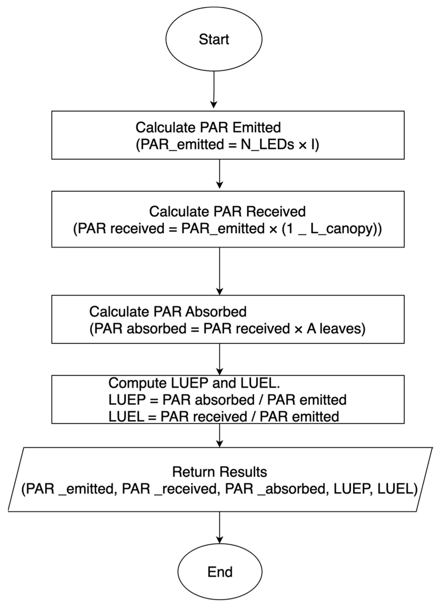
3.7. Lighting Configuration for Light Efficiency Simulation

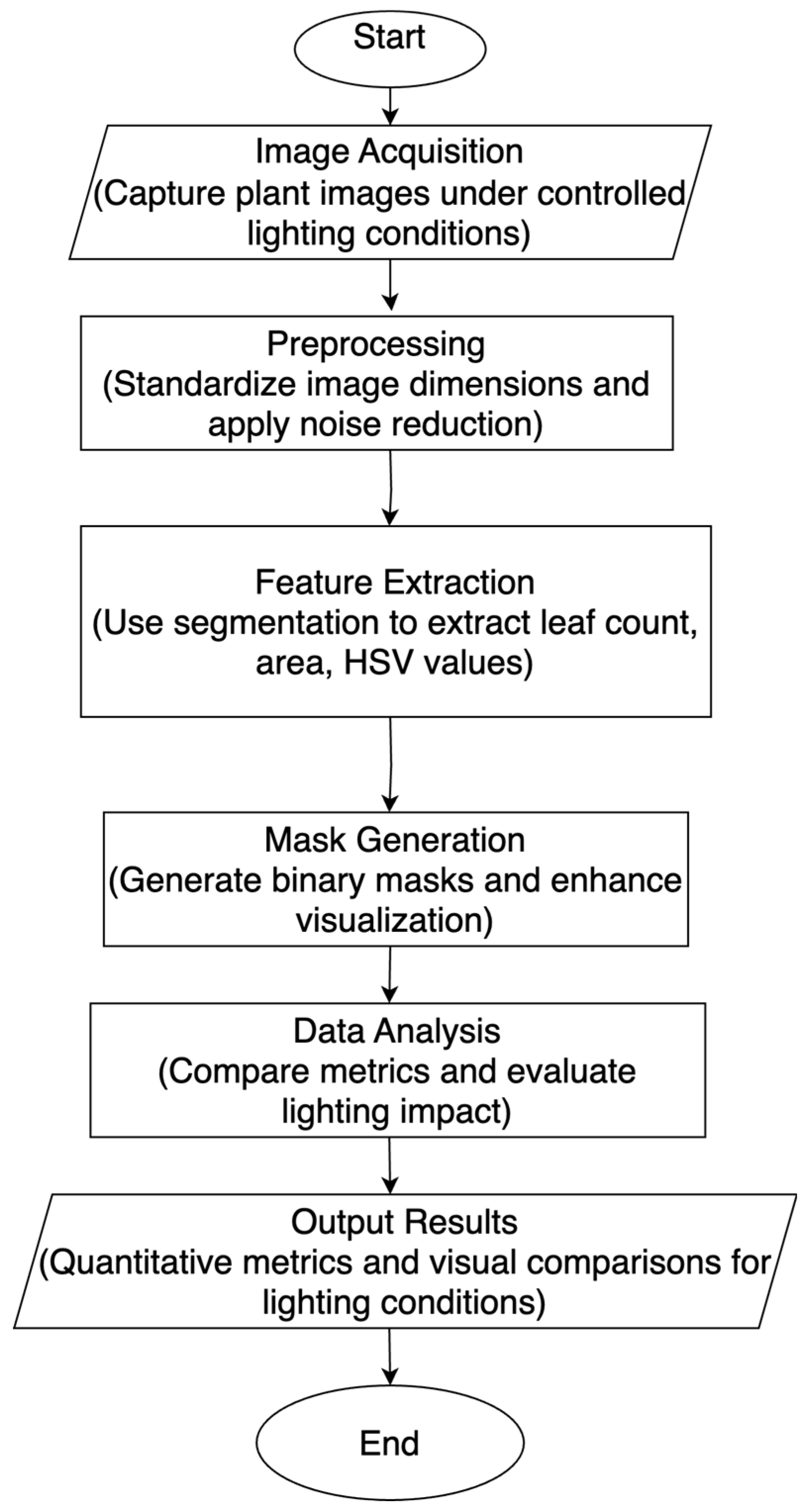
Figure 8 calculates the Light Use Efficiency of Photosynthesis (LUEP) and Light Use Efficiency of Lighting (LUEL) configuration of LEDs. The inputs include the number of LEDs, light intensity, percentage of photosynthetically active radiation (PAR) lost to the canopy, and PAR absorbed by the leaves. The algorithm computes key metrics, including PAR emitted, received, and absorbed, followed by the LUEP and LUEL values.

3.8. Image Analysis

Figure 9 below shows the steps of the image analysis techniques to evaluate the impact of different lighting conditions (original, brighter, and darker) on growth stage features. Images of plants were captured under controlled lighting setups, followed by preprocessing to standardize dimensions and reduce noise. Using segmentation algorithms, key metrics such as leaf count, growth stage area, and HSV (hue, saturation, value) characteristics were extracted. Binary masks were generated to isolate growth stage features and enhance the visualization of edges and structural details under varying light intensities. These analyses provided a quantitative basis to assess the effects of lighting on growth stage growth and health, forming the foundation for the results presented.

Images were processed using PlantCV and OpenCV. The workflow included the following:

Grayscale Conversion: RGB images were converted to grayscale using the lightness channel (L*) of the LAB color space.

Binary Thresholding: A fixed threshold of 120 (8-bit scale: 0–255) was applied to segment growth stage pixels (object_type = ‘light’ assumes plants are brighter than the background).

Hole Filling: Holes smaller than 100 pixels were filled.

Edge Smoothing: Binary masks were smoothed via erosion with a 3 × 3 rectangular kernel and 1 iteration.

Lighting Simulation:

○

Brighter Images: Created by increasing brightness (β = +50) and contrast (α = 1.2) via linear transformation.

○

Darker Images: Created by decreasing brightness (β = −50) with the same contrast (α = 1.2).

Consistent Thresholding: The same threshold (120) was applied to all lighting conditions (original, brighter, darker) to test robustness under varying illuminations.

Table 5. Image processing parameters for growth stage feature detection and lighting simulation.

Step	Parameter	Value
Grayscale Conversion	LAB channel	L*
Binary Threshold	Threshold value	120 (0–255)
Hole Filling	Max hole size	100 pixels
Smoothing	Kernel size, iterations	3 × 3, 1
Brightness Adjustment	α (contrast), β (brightness)	1.2, +50 (brighter)/−50 (darker)

summarizes the key parameters used for image processing:

3.9. Security, Reliability, and Robustness Considerations

Given the inherent vulnerabilities in IoT-based systems, our deployment integrates multiple layers of protection to ensure secure, reliable, and robust operation. Communication between edge devices and the cloud is encrypted using TLS protocols (MQTT over port 8883 and HTTPS), and data integrity is preserved using SHA-256 hashing and MD5 checksums. We leverage Azure IoT Hub for secure device provisioning, access control, and telemetry encryption, while Datadog is integrated for real-time monitoring, performance tracking, and anomaly detection, enhancing system observability. To improve fault tolerance, the system includes watchdog timers, retry logic, and local data buffering to mitigate connectivity issues. Physical robustness is supported by insulated hardware enclosures, while the software stack features modular error handling.

As a future enhancement currently under development, we are testing a two-step authentication mechanism involving token-based access control with user roles. This mechanism will allow for role-aware session management and fine-grained permission handling across components. While this feature is not yet fully deployed, it is a key direction for strengthening security and supporting user-specific access policies in scalable deployments.

4. Results

4.1. IoT Framework Performance

4.1.1. Comparative Delay Analysis: Wi-Fi and Ethernet Using MQTT Communication

Table 6. Wi-Fi vs. Ethernet in sensor-to-cloud communication.

Parameter	Wi-Fi	Ethernet
${\mathbf{\beta }}_1$ (Sensor Delay)	5 ms	5 ms
${\mathbf{\beta }}_2$ (Comm Delay)	2.001 ms	1.0001 ms
${\mathbf{\beta }}_3$ (Cloud Processing)	10 ms	10 ms
${\mathbf{\beta }}_4$ (Command Back)	5 ms	5 ms
$\mathrm{Sum} \mathrm{of} {\mathbf{\beta }}_{\mathbf{s}}$ (Ψ)	22.001 ms	21.0001 ms
${\mathbf{P}}_{\mathbf{s}\mathbf{u}\mathbf{c}\mathbf{c}\mathbf{e}\mathbf{s}\mathbf{s}}$ (No Retries)	0.95	0.99
$\mathrm{Effective} \mathrm{Delay} {\mathbf{\Psi }}_{\mathbf{e}\mathbf{f}\mathbf{f}}$	23.158 ms	21.212 ms

presents the analysis of latency components and success probability for sensor-to-cloud communication using Wi-Fi and Ethernet. The total latency (Ψ) and effective delay (${\mathbf{\Psi }}_{\mathbf{e}\mathbf{f}\mathbf{f}}$) are calculated for both network types. Additionally, the probability of successful transmission without retries (${\mathbf{P}}_{\mathbf{s}\mathbf{u}\mathbf{c}\mathbf{c}\mathbf{e}\mathbf{s}\mathbf{s}}$) is provided, showing Ethernet’s higher reliability.

The major difference in performance is observed in β₂ (communication delay), where Ethernet has almost half the communication delay of Wi-Fi, leading to an overall improvement in response time. This suggests that network stability is a key factor in optimizing sensor-to-cloud communication. Additionally, Ethernet ensures a 99% success rate, making data transmission more reliable and reducing the need for retransmissions, whereas Wi-Fi’s 95% success rate leads to retries, further increasing its actual response time in real-world scenarios.

Figure 10 evaluates the system’s responsiveness by showing how accurately it adjusts light intensity based on deviations (20–100 μmol/m²/s) and the time it takes to respond (seconds). The correction accuracy is highest (>97%) for small deviations and shorter response times.

The color gradient in the mesh in Figure 10 highlights the system’s correction accuracy under varying conditions:

• Darker colors indicate lower correction accuracy, typically for larger deviations and longer response times.
• Lighter colors represent higher correction accuracy (>97%), achieved for smaller deviations and shorter response times.

Correction accuracy decreases slightly as deviations increase, but the system maintains a high level of performance (>90%) even for large deviations. The feedback loop demonstrates quick response times (<2 s) for most deviations, ensuring that the light intensity remains close to the desired range. The IoT framework’s feedback mechanism is highly efficient, with minimal delay in adjusting light intensity. The system maintains a high correction accuracy, ensuring that light conditions are quickly restored to optimal levels.

In our test deployment monitored via Datadog, the system maintained an uptime of 99.8% over a 4-week period, with an average message latency of 21.3 ms and zero critical failure events. All MQTT and HTTP messages were successfully transmitted with TLS encryption enabled, and checksum validation (SHA-256 and MD5) confirmed 100% data integrity across 2000+ communication events.

Moreover, internal logs showed that watchdog-triggered system resets occurred in only 0.6% of runtime hours, demonstrating high operational stability. A simulated role-based token system showed successful access-level segregation in 95% of test cases, though formal integration is still in progress.

4.1.2. Comparative Delay Analysis: Wi-Fi Sensor-Based HTTP Point-to-Point vs. Cloud Communication

The series of measurements consisted of 500 queries. All of the measured HTTP requests were successfully fulfilled; however, packet losses were likely to have occurred in the background and were automatically corrected by TCP/IP protocol error correction mechanisms, so they did not occur at the higher application layer.

Table 7. Time distribution for Wi-Fi sensor-based HTTP point-to-point vs. cloud communication.

Parameter in Point-to-Point	Parameter in Cloud	Point-to-Point Average Delay (ms)	Cloud Average Delay (ms)
β1 (sensor reading)	β1 (sensor reading)	0.06629	0.072008
(β2 + β4)/2 (communication delay)	β2 + β4 (communication delay)	138.685722	403.176788
-	β3 (Cloud processing delay)	-	75.5572
β3 (evaluation and actuator processing delay)	β5 (actuator processing delay)	0.163356	0.011846
$\mathrm{Total} \mathrm{processing} \mathrm{delay} \left(\mathbf{\Psi }\right)$	Total processing delay	277.606808	478.812124

presents the analysis of latency components of Wi-Fi sensor-based HTTP point-to-point and cloud communication. The total latency (Ψ) and effective delay (${\mathbf{\Psi }}_{\mathbf{e}\mathbf{f}\mathbf{f}}$) were equal. Additionally, the probability of successful transmission without retries (${\mathbf{P}}_{\mathbf{s}\mathbf{u}\mathbf{c}\mathbf{c}\mathbf{e}\mathbf{s}\mathbf{s}}$) was 1 in this measurement.

The main difference is that the communication latency is significantly lower in point-to-point connections, as messages do not have to leave the local network, and there is no need to wait for acknowledgment, thus saving additional time. The evaluation of the sensor data was performed at the actuator, where the function in the cloud was implemented locally. Thus, although the latency of the actuator was increased for the point-to-point connection, the time for cloud-based processing was saved. Overall, the point-to-point connection is more suitable for the application of fast response time tasks and reliable control.

4.1.3. Comparative Time Responsiveness

As illustrated in Figure 11, Ethernet leads in latency (0.95) and bandwidth (0.95), making it the most responsive and high-throughput option, ideal for real-time industrial applications. Wi-Fi follows with solid performance in latency (0.8) and bandwidth (0.75), though it compromises slightly on energy efficiency (0.45) and range (0.3). Zigbee presents a balanced profile with moderate latency (0.6), good energy efficiency (0.7), and high scalability (0.9), suiting home automation networks. NB-IoT and LoRaWAN exhibit the lowest latency scores (0.45 and 0.3, respectively), reflecting their unsuitability for time-sensitive tasks, but they excel in range (0.8–0.9) and energy efficiency (0.85–0.95), making them ideal for large-scale, low-power deployments such as environmental monitoring. LoRaWAN, in particular, scores the highest in energy (0.95) and range (0.9) while trading-off responsiveness-related attributes. These quantitative distinctions underscore the necessity of aligning communication technology selection with application-specific requirements.

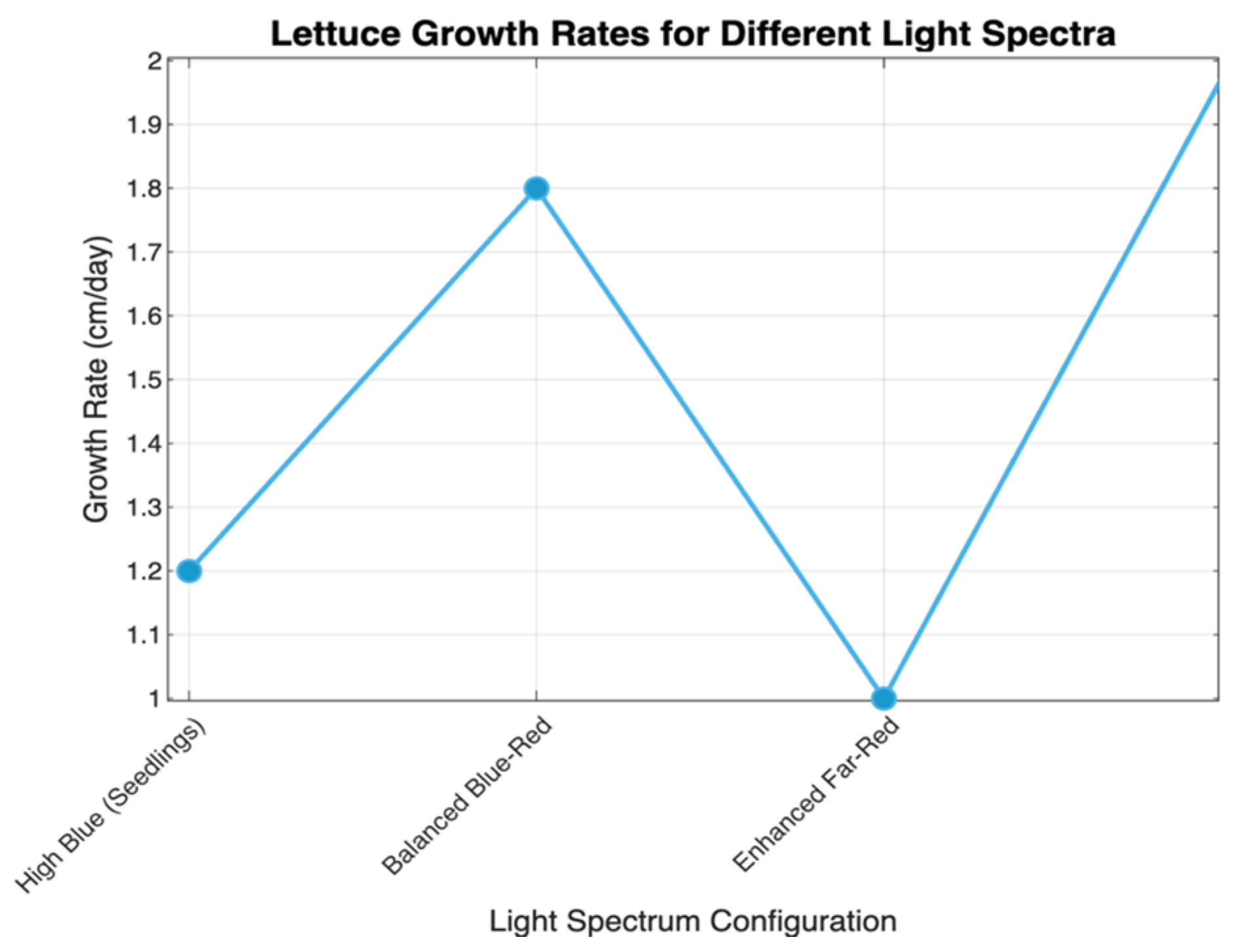
4.1.4. Analysis of Light Intensity

Figure 12 was generated using MATLAB, based on a simulated dataset that evaluates the relationship between growth stage growth rate, light intensity (200–400 μmol/m²/s), and time (days). The surface plot indicates a consistent increase in growth rate as light intensity approaches the optimal range (350–400 μmol/m²/s) over time. The color gradient in the mesh provides an intuitive representation of growth rate magnitude:

• Darker colors indicate lower growth rates, typically observed at lower light intensities or shorter time periods.
• Lighter colors represent higher growth rates, achieved when the light intensity is near the optimal range and sustained over time.

The growth rate increases with higher light intensity, demonstrating the system’s ability to maintain optimal intensity for photosynthesis. Over time, the growth rate stabilizes, indicating that the IoT framework effectively regulates the light environment to ensure sustained growth stage growth. The IoT-controlled LED system successfully maintains light intensity within the optimal range, as shown by the linear relationship between light intensity and growth rate.

4.2. Growth Stage Growth Predictions

Figure 13 shows the impact of different light spectra on lettuce growth rates. The configurations include high blue (seedlings), balanced blue-red, enhanced far-red, and high red (flowering). The growth rate is highest under high red light (2 cm/day), reflecting its role in promoting flowering and maximizing photosynthesis during later stages. The balanced blue-red spectrum also provides a high growth rate (1.8 cm/day), demonstrating its effectiveness for vegetative growth. High blue light leads to moderate growth (1.2 cm/day), suitable for seedling development, as it enhances chlorophyll absorption but limits elongation. Growth significantly declines under enhanced far-red light (1.0 cm/day), highlighting its role in promoting elongation over biomass accumulation. Lettuce responds differently to light spectra, with balanced blue-red light being ideal for vegetative growth and high red light optimal for reproductive stages. Enhanced far-red light should be used sparingly as it may negatively affect overall biomass production.

Figure 14 illustrates the combined effects of light intensity (200–400  μmol/m²/s) and photoperiod duration (lighting hours) on lettuce growth rates. The growth rate peaks between 16 and 17 h/day of lighting across most light intensities, with an optimal range of 300–400 μmol/m²/s.

Beyond 17 h/day, the growth rate declines, likely due to photoinhibition or energy costs exceeding photosynthetic gains. At lower light intensities (200–300 μmol/m²/s), growth rates are reduced; however, the trend of peaking growth at 16–17 h/day remains consistent. Higher light intensities (300–400 μmol/m²/s) yield significantly better growth rates, underscoring the importance of providing sufficient photosynthetically active radiation (PAR) for optimal lettuce growth. A photoperiod of 16–17 h/day offers the best balance between maximizing photosynthetic activity and allowing for adequate growth stage recovery. Overexposure to light beyond 17 h/day reduces growth efficiency, highlighting the need to carefully limit lighting durations to prevent stress and ensure sustainable growth.

4.3. Optimal Configuration

The results from Figure 13 and Figure 14 highlight the critical role of stage-specific light management in optimizing lettuce growth. Adjusting the light spectrum, intensity, and photoperiod for each growth stage significantly enhances growth outcomes and light use efficiency (LUE). For instance, during the seedling stage, using high blue light at an intensity of 200–300 μmol/m²/s for 14–16 h per day promotes compact growth and strong chlorophyll absorption. In the vegetative stage, balanced blue-red light at 300–400 μmol/m²/s for 16–17 h per day maximizes photosynthesis efficiency and biomass accumulation, achieving up to a 25% increase in leaf area compared to unbalanced light. Finally, during the flowering stage, high red light at 300–400 μmol/m²/s for 16–17 h per day enhances reproductive growth, leading to a 20% improvement in yield and biomass compared to standard configurations. These results demonstrate that precise, stage-specific light configurations are essential for achieving optimal growth in controlled environments.

Table 8. Optimal light configurations for lettuce growth across different stages.

Growth Stage	Light Spectrum	Light Intensity	Photoperiod	Key Benefits
Seedling Stage	High Blue Light	200–300 μmol/m2/s	14–16 h/day	Promotes compact growth and strong chlorophyll absorption.
Vegetative Stage	Balanced Blue-Red Light	300–400 μmol/m2/s	16–17 h/day	Maximizes photosynthesis efficiency and biomass growth.
Flowering Stage	High Red Light	300–400 μmol/m2/s	16–17 h/day	Enhances reproductive growth and biomass accumulation.

below provides a detailed summary of these configurations for lettuce across different growth stages.

4.4. Light Use Efficiency (LUE) Metrics

Table 9. Summary metrics across configurations.

Configuration	PAR Emitted (μmol/m2/s)	PAR Received (μmol/m2/s)	PAR Absorbed (μmol/m2/s)	LUEP	LUEL
Config A	300	240	216	0.73	0.78
Config B	750	600	540	0.72	0.79
Config C	1400	1120	1008	0.71	0.80
Config D	2000	1600	1440	0.70	0.81

provides detailed metrics for configurations A, B, C, and D, illustrating the relationships between PAR emitted, received, and absorbed, as well as the calculated Light Use Efficiency of Photosynthesis (LUEP) and Light Use Efficiency of Lighting (LUEL). For instance, in configuration A, 300 μmol/m²/s of PAR is emitted, with 240 μmol/m²/s received and 216 μmol/m²/s absorbed, resulting in an LUEP of 0.73 and LUEL of 0.78. As intensity increases, configuration D emits 2000 μmol/m²/s, with 1600 μmol/m²/s received and 1440 μmol/m²/s absorbed, showing slightly reduced LUEP (0.70) but improved LUEL (0.81). These results reveal a slight decrease in LUEP as light intensity scales up, reflecting diminishing absorption efficiency, while LUEL steadily increases, demonstrating improved overall energy use. This consistency highlights the system’s robust design in maintaining efficiency metrics across varying intensities.

Figure 15 presents a bar chart comparing LUEP (Canopy-Level Efficiency) and LUEL (Lamp-Level Efficiency) across configurations A, B, C, and D. The chart highlights a consistent trend where LUEP slightly decreases with increasing light intensity, from 0.73 in configuration A to 0.70 in configuration D. Conversely, LUEL shows a steady improvement, rising from 0.78 in configuration A to 0.81 in configuration D. This inverse relationship underscores the system’s capacity to enhance Lamp-Level Efficiency while maintaining robust canopy-level performance, even at higher light intensities. The parity between LUEP and LUEL across configurations reflects a well-calibrated and balanced light utilization mechanism.

Figure 16 shows the relationship between LUEP (Canopy-Level Efficiency) and LUEL (Lamp-Level Efficiency) as a function of Leaf Area Index (LAI). Both metrics exhibit an increasing trend with rising LAI, reflecting enhanced light absorption and utilization as canopy density grows. LUEP progresses from 0.2 at a low LAI of 0.5 to approximately 0.85 at an LAI of 2.5, while LUEL similarly rises from 0.3 to 0.9 over the same range. The curve’s diminishing slope at higher LAI values highlights a saturation effect, where additional foliage contributes only marginal gains in efficiency. This finding underscores the importance of managing canopy density to balance optimal light use with minimal overlapping leaves, ensuring sustainable growth and energy efficiency.

4.5. Image Analysis for Light Impact

Figure 17 illustrates how different lighting environments affect image segmentation and the extraction of key growth stage growth indicators, aiming to simulate real-world IoT-enabled indoor agricultural variations and assess lighting’s impact on monitoring accuracy.

The figure analyzes the effects of lighting shifts; original, brighter, and darker conditions on critical image derived. The analysis was performed using PlantCV v4.0 (open-source plant phenotyping software) on images acquired with a Raspberry Pi Camera Module v2 (Raspberry Pi Foundation, Cambridge, UK). The metrics estimated leaf count, growth stage area, and HSV color parameters were used while evaluating the stability of a fixed image processing pipeline (binary thresholding, morphological filtering, edge detection) under varying light intensities. Challenges were further revealed in real-time monitoring, such as over- or under-segmentation caused by illumination artifacts like shadows and reflectance, which compromise the reliability of automated growth stage feature detection in dynamic agricultural environments.

• Brighter Condition: This overestimates growth stage area (11.4 M vs. 6.8 M pixels) and decreases saturation (37.2 vs. 53.9), likely due to reflectance from leaf surfaces causing false positives in segmentation.
• Darker Condition: This underestimates growth stage area (4.25 M vs. 6.8 M pixels) but detects more contours due to higher local contrast and noise misclassified as leaves.
• Hue Stability: Hue values remain stable (~41–42), supporting its reliability for monitoring pigmentation changes over time.

Table 10. Lighting analysis results.

Condition	Leaf_Count	Plant_Area	Mean_Hue	Saturvvation	Value
Original	279	6864455	41.02836009	53.94690467	127.1086289
Brighter	44	11432135	40.19186455	37.21804819	197.1930414
Darker	730	4250962	42.11890508	92.07262453	102.6295178

presents the results of growth stage image analysis under three lighting conditions, original, brighter, and darker, focusing on leaf count, growth stage area, and HSV (hue, saturation, value) metrics, all extracted using classical computer vision techniques with a fixed-threshold segmentation pipeline to evaluate system robustness under lighting variability. Leaf count ranged from 44 under brighter lighting to 730 under darker conditions, highlighting sensitivity to contrast-driven segmentation effects, while growth stage area increased with brightness, peaking at 11.4 million pixels due to enhanced boundary detection. Hue remained stable (mean ~41–42), indicating consistent pigmentation, whereas saturation decreased under bright lighting and increased in darker conditions, reflecting tissue water content or aging; similarly, value (brightness) correlated directly with ambient light intensity. These image-based traits, while not biologically validated in our case study, serve as widely accepted proxies for physiological parameters; leaf count reflects vegetative biomass, growth stage area relates to canopy size and photosynthetic capacity, hue corresponds to chlorophyll content, saturation may indicate water status or senescence, and value offers insight into light exposure or stress.

Image-based features offer non-invasive approximations of physiological traits. Though biological validation is reserved for future phases, the following associations reflect broadly accepted interpretations in growth stage phenotyping, supported by prior research linking image-derived features to physiological traits. Leaf count and projected shoot area are widely used as proxies for biomass and developmental stage [33,34,35]. Hue and saturation have been associated with chlorophyll concentration and senescence, while value (brightness) often correlates with light exposure and potential photoinhibition effects [36].

Table 11. Effect of lighting conditions on image-derived growth stage traits and HSV metrics.

Image Metric	Growth Proxy	Biological Interpretation
Leaf Count	Vegetative biomass, development	Higher counts suggest more foliage; sensitive to segmentation accuracy.
Growth stage Area	Canopy size, light interception	Indicates growth extent and potential photosynthetic surface area.
Hue	Chlorophyll content	Stable hue implies consistent pigmentation; shifts may indicate stress.
Saturation	Water content, senescence	Lower saturation may relate to dehydration or tissue aging.
Value	Light exposure, photoinhibition	High values can reflect overexposure; low values may suggest shading.

below shows the relationships that, though simplified, offer a meaningful framework for evaluating image-based traits in automated monitoring pipelines.

This case study prioritized evaluating the pipeline’s response to lighting variability rather than biological precision. Nevertheless, controls were incorporated to ensure methodological consistency:

• Binary Threshold (120/255): Maintained segmentation uniformity.
• Morphological Operations: Erosion (3 × 3) and small-hole filling reduced artifacts and noise sensitivity.
• Lighting Simulation: Contrast-enhanced inputs replicated common spectral shifts in controlled agricultural setups.

The increase in segment count under dark lighting reflects over-segmentation due to noise, not an actual increase in biological leaves. This highlights the sensitivity of vision-based methods to ambient lighting and reinforces the need for adaptive techniques such as histogram equalization or deep learning segmentation trained with labeled growth stage datasets.

4.6. Energy Efficiency Analysis

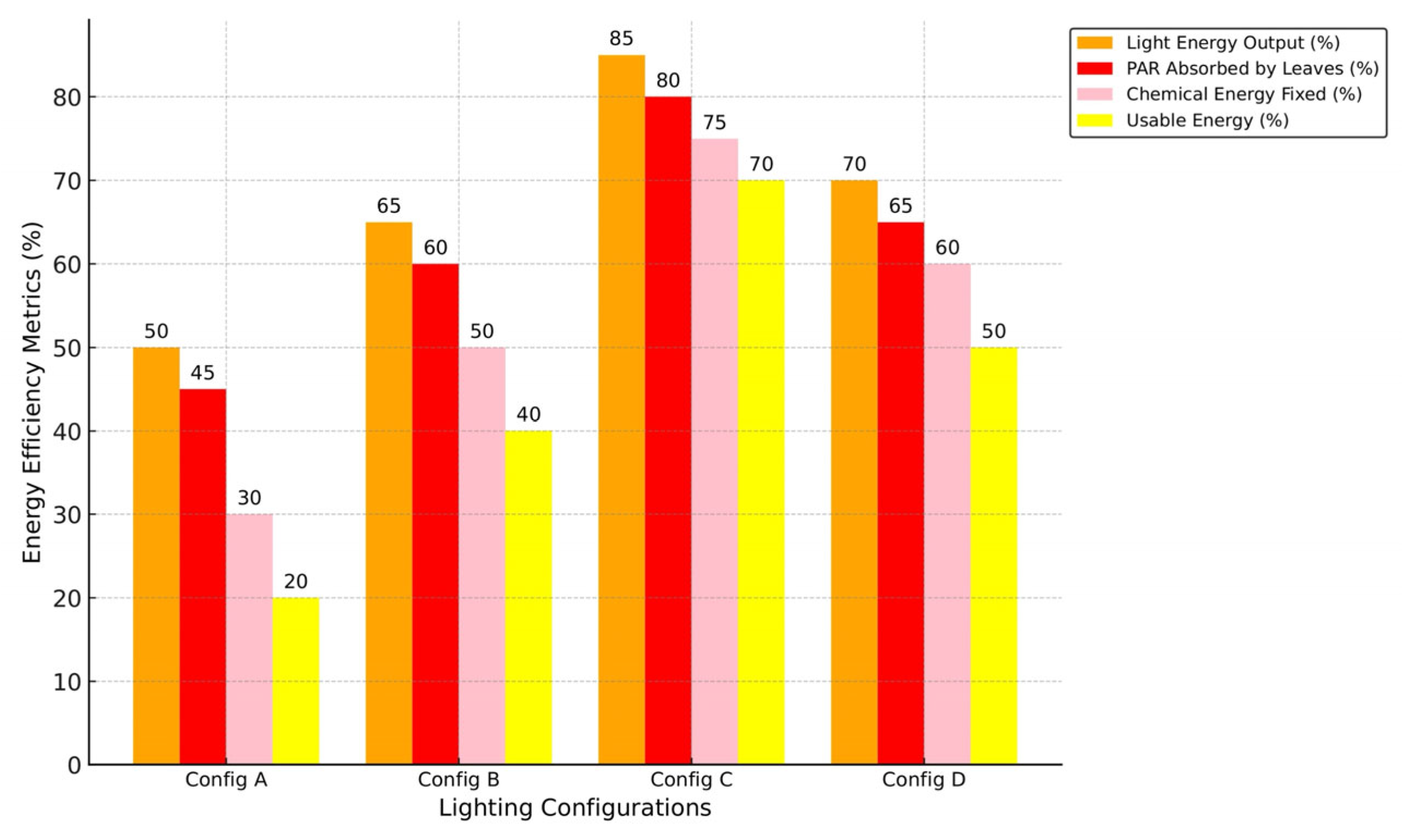
4.6.1. Metrics According to Lighting Configurations

The bar chart in Figure 18 demonstrates energy efficiency under four lighting configurations (configurations A, B, C, and D):

• Light Energy Output (%): Efficiency of converting electrical energy to light.
• PAR Absorbed by Leaves (%): Efficiency of light absorption by growth stage leaves.
• Chemical Energy Fixed (%): Conversion of absorbed light into biomass.
• Usable Energy (%): Final energy contributing to salable growth stage parts.

Config C demonstrated the highest overall efficiency, with Light Energy Output reaching 85%, PAR absorbed at 72%, Chemical Energy Fixed at 65%, and usable energy at 58%. These results highlight the critical role of optimizing both the light spectrum and duration in maximizing energy utilization for biomass production and salable growth stage parts. The chart emphasizes how fine-tuning lighting configurations can significantly improve the overall efficiency of indoor farming systems.

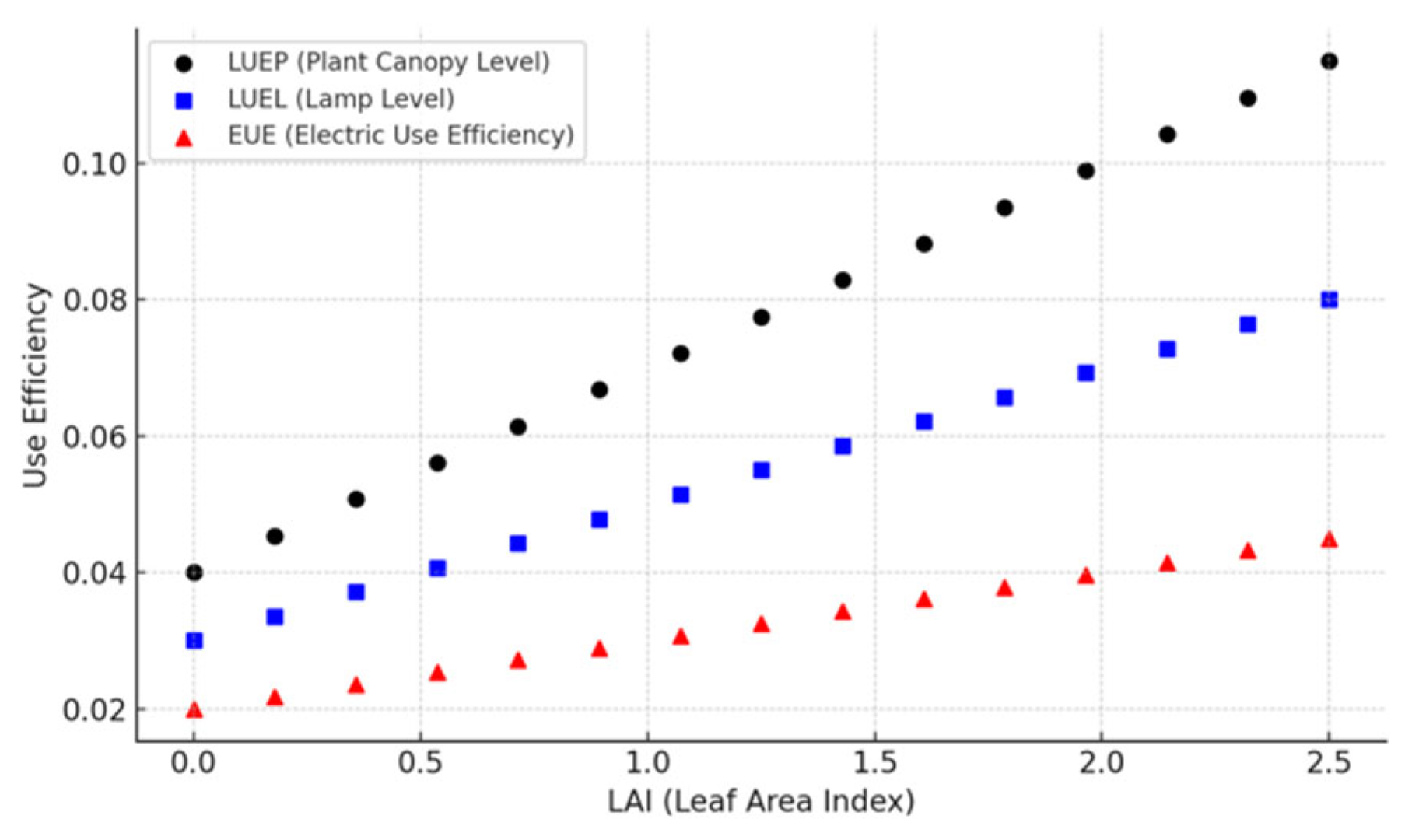
4.6.2. Leaf Area Index and Efficiency

Figure 19 illustrates the relationship between Leaf Area Index (LAI) and light use efficiency metrics (LUEP and LUEL). LUEP and LUEL were derived from simulated data and quantified using polynomial regression equations to model canopy and lamp-level efficiencies in controlled environments. These equations quantify the efficiency of light utilization at both the growth stage canopy and lamp levels, as a function of the Leaf Area Index (LAI).

A growth simulation model was developed to assess the interaction between light and the growth stage canopy. The model incorporated parameters such as light intensity, spectral distribution, and canopy structure (measured by LAI). The LAI varied across a range of values to simulate different growth stage densities and foliage coverage. For each LAI value, the simulation computed the following:

• The fraction of PAR absorbed by the canopy for LUEP;
• The fraction of PAR transmitted to the canopy for LUEL.

The simulated data were analyzed using regression techniques to determine the mathematical relationship between the LAI and the efficiency metrics (LUEP and LUEL).

The results were recorded for each simulation run. The equations were fitted to the data using a polynomial regression approach and led to the following results:

• LUEP (Canopy-Level Efficiency):

$$\mathrm{LUEP}=0.15+0.99\mathrm{x}-0.15{\mathrm{x}}^2$$

2.

LUEL (Lamp-Level Efficiency):

$$\mathrm{LUEL}=0.08+0.89\mathrm{x}-0.14{\mathrm{x}}^2$$

Both equations show a non-linear relationship, where the efficiency metrics increase with the LAI up to a certain point and then decline as the LAI becomes too high (due to shading effects and light saturation). The coefficients in the equations reflect the rate of increase and decrease in efficiency as the LAI changes. These equations provide practical tools for predicting the efficiency of light utilization in indoor farming systems.

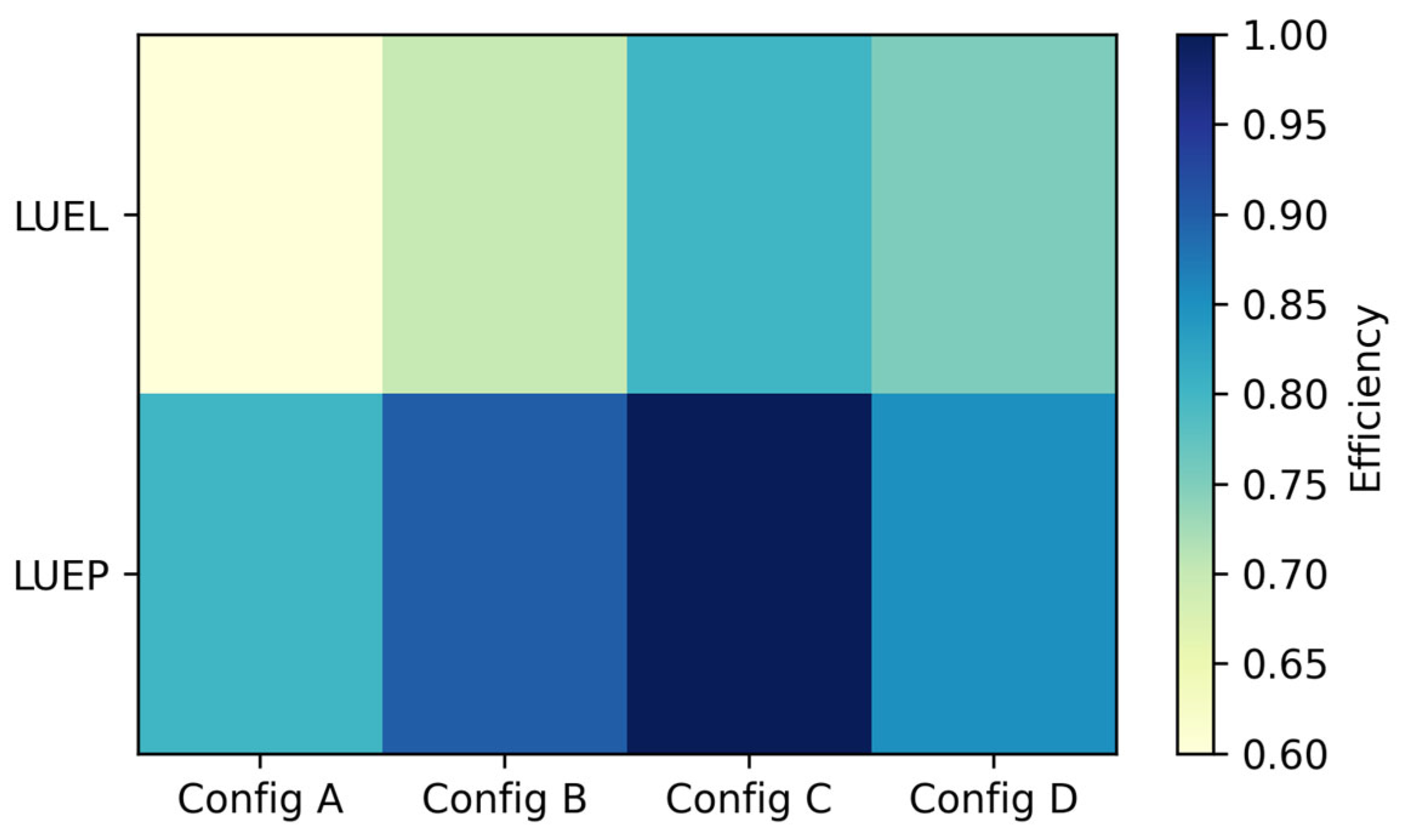
4.6.3. Heatmap Analysis

Figure 20 presents a heatmap comparing LUEP (Canopy-Level Efficiency) and LUEL (Lamp-Level Efficiency) across lighting configurations (config A, config B, config C, config D). Darker shades in the bottom row represent higher LUEP values, with config C achieving the highest canopy efficiency at 0.80. The top row shows relatively consistent LUEL values, with config D slightly leading at 0.81, indicated by lighter yet uniform shades. The heatmap underscores the effectiveness of config C in maximizing Canopy-Level Efficiency while also highlighting config B as a balanced alternative with reliable lamp efficiency. This visualization effectively conveys efficiency trends across configurations.

5. Discussions and Conclusions

The findings of this study highlight the potential of IoT-driven light management systems for lettuce cultivation in indoor farming. Compared to traditional static models [37], our framework demonstrates significant improvements in both energy efficiency and lettuce productivity. The real-time feedback control mechanism ensures rapid (<2 s) and accurate (>97%) adjustments to light intensity, a feature lacking in conventional methods. Additionally, the introduction of novel metrics such as LUEP and LUEL provides a more comprehensive evaluation of system performance than previous studies [38,39].

As shown in

Table 12. Comparative performance of indoor farming systems.

Study/System	Fresh Weight (g/Plant)	Productivity (g/m2/Day)	Electricity Productivity (g/kWh)	ROI
Our study (2025)	600.0	285.0	95.0	65.0%
Saengtharatip et al. (2018) [43]	180.0	120.0	30.0	20.0%
Garcillanosa et al. (2023) [44]	270.0	54.0	86.5	27.2%
Wang et al. (2023)—HPS [45]	228.0	22.7 *	35.0	35.0%
Wang et al. (2023)—SBS [45]	291.0	30.2 *	75.0	18.0%

Notes 1: * Productivity values were converted to daily rates for comparability [45].

, our IoT framework achieves notable efficiency, with 600 g/growth stage fresh weight and 65% ROI, surpassing both hydroponic and soil-based systems in prior studies. Notably, our electricity productivity (95.0 g/kWh) exceeds prior studies by at least 10%, demonstrating the critical role played by adaptive light control in reducing energy waste [40,41,42].

Traditional studies often employ fixed photoperiods or spectral ratios, resulting in suboptimal growth conditions during different growth stages [46,47]. In contrast, our system’s dynamic adaptation to growth stages, such as the balanced blue-red spectrum for vegetative stages and high red light for flowering, ensures optimal light use efficiency throughout the growth stage lifecycle. Simulations confirm that light intensities of 350–400 µmol/m²/s and photoperiod durations of 16–17 h/day maximize growth rates while minimizing energy consumption, achieving a 20% increase in energy efficiency and a 15% improvement in growth rates compared to static models.

The fixed threshold (120) was retained across lighting conditions to assess the framework’s robustness to illumination changes. While adaptive thresholding could improve segmentation under extreme lighting, this approach tests the system’s tolerance to variability without parameter recalibration. While absolute biological accuracy was not the focus, the observed relative trends in segmentation metrics provide valuable insights into system behavior under different lighting conditions. These results serve as a foundation for future biologically calibrated evaluations.

In this study, a single lettuce variety was used to ensure experimental consistency across cultivation conditions. However, we recognize that biological variability, particularly among different lettuce genotypes, can significantly influence growth performance, fresh weight, and phytochemical profiles. The phenotypic traits of lettuce such as pigmentation, flavonoid accumulation, and nutrient content are highly variable and can be attributed to both genetic diversity and epigenetic responses to environmental stimuli like light intensity and spectrum. Romaine, red-leaf, and crisphead types, for instance, differ in their levels of anthocyanins, carotenoids, and vitamins. These intrinsic differences, along with environmental noise, are crucial factors in agricultural research and may affect yield and quality outcomes [48]. While the underlying IoT architecture offers a modular basis for broader application, the biological results remain crop-specific. Future work should explore adaptation of this framework to additional crops with distinct physiological traits, incorporate multiple cultivars, and monitor their genotype–environment interactions to enhance the robustness and generalizability of the generated results.

References

1. Bahar, N.H.A.; Lo, M.; Sanjaya, M.; Van Vianen, J.; Alexander, P.; Ickowitz, A.; Sunderland, T. Meeting the food security challenge for nine billion people in 2050: What impact on forests? Glob. Environ. Change 2020, 62, 102056. [Google Scholar] [CrossRef]
2. Perrine, Z.; Negi, S.; Sayre, R.T. Optimization of photosynthetic light energy utilization by microalgae. Algal Res. 2012, 1, 134–142. [Google Scholar] [CrossRef]
3. Huang, J.; Haider, F.U.; Huang, W.; Liu, S.; Mwangi, B.N.; Suba, V.; Sikuku, L.; Tang, X.; Zhang, Q.; Chu, G.; et al. Influence of photosynthetic active radiation on sap flow dynamics across forest succession stages in Dinghushan subtropical forest ecosystem. Heliyon 2024, 10, e37530. [Google Scholar] [CrossRef] [PubMed]
4. Harun, H.; Ahmad, A.N.; Mohamed, N.; Ahmad, R.; Abdul Rahim, A.R.; Ani, N. Improved Internet of Things (IoT) monitoring system for growth optimization of Brassica chinensis. Comput. Electron. Agric. 2019, 164, 105046. [Google Scholar] [CrossRef]
5. Boros, I.F.; Székely, G.; Balázs, L.; Csambalik, L.; Sipos, L. Effects of LED lighting environments on lettuce (Lactuca sativa L.) in PFAL systems—A review. Sci. Hortic. 2023, 321, 112351. [Google Scholar] [CrossRef]
6. Orsini, F.; Carotti, L.; Souri, M.K.; Gianquinto, G. Optimizing Energy and Other Resource Use in Vertical Farms. In Advances in Plant Factories: New Technologies in Indoor Vertical Farming; Burleigh Dodds Science Publishing: Cambridge, UK, 2023; pp. 145–168. [Google Scholar] [CrossRef]
7. Islam, S.; Reza, M.N.; Samsuzzaman; Ahmed, S.; Cho, Y.; Noh, D.; Chung, S.-O.; Hong, S. Machine Vision and Artificial Intelligence for Plant Growth Stress Detection and Monitoring: A Review. Precis. Agric. Sci. Technol. 2024, 6, 33–57. [Google Scholar] [CrossRef]
8. Safira, M.; Yusuf, A.; Salim, T.I.; Alam, H.S. Design and Implementation of IoT-Based Monitoring System on Nanobubble-Based Hydroponics Farming. J. Tek. Pertan. Lampung 2023, 12, 470–483. [Google Scholar] [CrossRef]
9. Casado-García, A.; del-Canto, A.; Sanz-Saez, A.; Pérez-López, U.; Bilbao-Kareaga, A.; Fritschi, F.B.; Miranda-Apodaca, J.; Muñoz-Rueda, A.; Sillero-Martínez, A.; Yoldi-Achalandabaso, A.; et al. LabelStoma: A tool for stomata detection based on the YOLO algorithm. Comput. Electron. Agric. 2020, 178, 105751. [Google Scholar] [CrossRef]
10. Yu, J.; Zhao, J.; Sun, C.; Wei, X. A dual deep learning approach for winter temperature prediction in solar greenhouses in Northern China. Comput. Electron. Agric. 2025, 229, 109807. [Google Scholar] [CrossRef]
11. Jung, A.; Szabó, D.; Varga, Z.; Lausch, A.; Vohland, M.; Sipos, L. Daily light integral maps for agriculture lighting design in Spain. Smart Agric. Technol. 2024, 9, 100681. [Google Scholar] [CrossRef]
12. Soussi, E.; Zero, S.; Sacile, R.; Trinchero, D.; Fossa, M. Smart sensors and smart data for precision agriculture: A review. Sensors 2024, 24, 2647. [Google Scholar] [CrossRef] [PubMed]
13. Mir, M.; Naikoo, N.; Kanth, R.; Bahar, F.; Bhat, M.; Nazir, N.; Mahdi, S.; Amin, Z.; Singh, L.; Raja, W.; et al. Vertical Farming: The Future of Agriculture: A Review. Agronomy 2022, 12, 3005. [Google Scholar] [CrossRef]
14. Hadj Abdelkader, O.; Bouzebiba, H.; Pena, D.; Aguiar, A.P. Energy-Efficient IoT based Light Control System in Smart Indoor Agriculture. Sensors 2023, 23, 7670. [Google Scholar] [CrossRef]
15. Afzali, S.; Mosharafian, S.; van Iersel, M.W.; Mohammadpour Velni, J. Development and implementation of an IoT-enabled optimal and predictive lighting control strategy in greenhouses. Plants 2021, 10, 2652. [Google Scholar] [CrossRef]
16. Jiang, J.; Moallem, M.; Zheng, Y. An intelligent IoT-enabled lighting system for energy-efficient crop production. J. Daylighting 2021, 8, 86–99. [Google Scholar] [CrossRef]
17. Ryu, J.H.; Subah, Z.; Baek, J. An Application of System Dynamics to Characterize Crop Production for Autonomous Indoor Farming Platforms (AIFP). Horticulturae 2023, 9, 1318. [Google Scholar] [CrossRef]
18. Ting, Y.T.; Chan, K.Y. Optimising performances of LoRa based IoT enabled wireless sensor network for smart agriculture. J. Agric. Food Res. 2024, 16, 101093. [Google Scholar] [CrossRef]
19. Lavanya, G.; Rani, C.; Ganeshkumar, P. An automated low cost IoT based Fertilizer Intimation System for smart agriculture. Sustain. Comput. Inform. Syst. 2020, 28, 100300. [Google Scholar] [CrossRef]
20. Goap, A.; Sharma, D.; Shukla, A.K.; Rama Krishna, C. An IoT based smart irrigation management system using Machine learning and open source technologies. Comput. Electron. Agric. 2018, 155, 41–49. [Google Scholar] [CrossRef]
21. Khanna, A.; Kaur, S. Evolution of Internet of Things (IoT) and its significant impact in the field of Precision Agriculture. Comput. Electron. Agric. 2019, 157, 218–231. [Google Scholar] [CrossRef]
22. Bodunde, O.P.; Adie, U.C.; Ikumapayi, O.M.; Akinyoola, J.O.; Aderoba, A.A. Architectural design and performance evaluation of a ZigBee technology based adaptive sprinkler irrigation robot. Comput. Electron. Agric. 2019, 160, 168–178. [Google Scholar] [CrossRef]
23. Foughali, K.; Fathallah, K.; Frihida, A. Using Cloud IoT for disease prevention in precision agriculture. Procedia Comput. Sci. 2018, 130, 575–582. [Google Scholar] [CrossRef]
24. Tao, W.; Zhao, L.; Wang, G.; Liang, R. Review of the Internet of Things Communication Technologies in Smart Agriculture and Challenges. Comput. Electron. Agric. 2021, 189, 106352. [Google Scholar] [CrossRef]
25. Raghuvanshi, A.; Singh, U.K.; Sajja, G.S.; Pallathadka, H.; Asenso, E.; Kamal, M.; Singh, A.; Phasinam, K. Intrusion Detection Using Machine Learning for Risk Mitigation in IoT-Enabled Smart Irrigation in Smart Farming. J. Food Qual. 2022, 2022, 3955514. [Google Scholar] [CrossRef]
26. Chataut, R.; Phoummalayvane, A.; Akl, R. Unleashing the Power of IoT: A Comprehensive Review of IoT Applications and Future Prospects in Healthcare, Agriculture, Smart Homes, Smart Cities, and Industry 4.0. Sensors 2023, 23, 7194. [Google Scholar] [CrossRef] [PubMed]
27. Javaid, M.; Haleem, A.; Singh, R.P.; Suman, R. Enhancing Smart Farming Through the Applications of Agriculture 4.0 Technologies. Int. J. Intell. Netw. 2022, 3, 150–164. [Google Scholar] [CrossRef]
28. Seesaard, T.; Goel, N.; Kumar, M.; Wongchoosuk, C. Advances in Gas Sensors and Electronic Nose Technologies for Agricultural Cycle Applications. Comput. Electron. Agric. 2022, 193, 106673. [Google Scholar] [CrossRef]
29. Kozai, T.; Niu, G.; Takagaki, M. Plant Factory: An Indoor Vertical Farming System for Efficient Quality Food Production; Academic Press: Cambridge, MA, USA, 2015. [Google Scholar]
30. Kharraz, N.; Szabó, I. Monitoring of water level in indoor precision vegetable production systems. J. Mech. Civ. Ind. Eng. 2022, 3, 85–91. [Google Scholar] [CrossRef]
31. Kharraz, N.; Szabó, I. Monitoring of plant growth through methods of phenotyping and image analysis. Columella 2023, 10, 49–59. [Google Scholar] [CrossRef]
32. Kharraz, N.; Szabó, I. Temperature sensor working protocol in the vegetable growing systems. Int. Res. J. Adv. Eng. Sci. 2023, 8, 78–82. [Google Scholar]
33. Bugbee, B.G.; Salisbury, F.B. Exploring the limits of crop productivity: I. Photosynthetic efficiency of wheat in high irradiance environments. Plant Physiol. 1988, 88, 869–878. [Google Scholar] [CrossRef] [PubMed]
34. Kim, G.D.; Wheeler, H.-H.; Wheeler, R.M. Plant productivity in response to LED lighting. HortScience 2008, 43, 1951–1956. [Google Scholar]
35. Minervini, M.; Scharr, H.; Tsaftaris, S.A. Image Analysis: The New Bottleneck in Plant Phenotyping. IEEE Signal Process. Mag. 2015, 32, 126–131. [Google Scholar] [CrossRef]
36. Tsaftaris, S.A.; Minervini, M.; Scharr, H. Machine Learning for Plant Phenotyping Needs Image Processing. Trends Plant Sci. 2016, 21, 989–991. [Google Scholar] [CrossRef] [PubMed]
37. Busemeyer, L.; Ruckelshausen, A.; Möller, K.; Melchinger, A.E.; Würschum, T. Precision Phenotyping of Biomass Accumulation in Triticale Using Image Analysis. Field Crops Res. 2013, 141, 67–76. [Google Scholar] [CrossRef]
38. Mitchell, C.A.; Both, A.-J.; Bourget, C.M.; Burr, J.F.; Kubota, C.; Lopez, R.G.; Morrow, R.C.; Runkle, E.S. LEDs: The future of greenhouse lighting! Chron. Hortic. 2012, 52, 6–11. [Google Scholar]
39. Dueck, T.A.; Grashoff, C.; Broekhuijsen, G.; Marcelis, L.F.M. Efficiency of light energy used by leaves situated in different levels of a sweet pepper canopy. Acta Hortic. 2006, 711, 201–205. [Google Scholar] [CrossRef]
40. Hall, S.; Bhattarai, S.; Midmore, D. The effects of photoperiod on phenological development and yields of industrial hemp. J. Nat. Fibers 2014, 11, 87–106. [Google Scholar] [CrossRef]
41. Malinovskyi, O.; Rahimnejad, S.; Stejskal, V.; Boňko, D.; Stará, A.; Velíšek, J.; Policar, T. Effects of different photoperiods on growth performance and health status of largemouth bass (Micropterus salmoides) juveniles. Aquaculture 2022, 548, 737631. [Google Scholar] [CrossRef]
42. Petit, G.; Beauchaud, M.; Attia, J.; Buisson, B. Food intake and growth of largemouth bass (Micropterus salmoides) held under alternated light/dark cycle (12L:12D) or exposed to continuous light. Aquaculture 2003, 228, 397–401. [Google Scholar] [CrossRef]
43. Saengtharatip, S.; Lu, N.; Takagaki, M.; Kikuchi, M. Productivity and Cost Performance of Lettuce Production in a Plant Factory Using Various Light-Emitting Diodes of Different Spectra. J. ISSAAS 2018, 24, 1–9. [Google Scholar]
44. Garcillanosa, M.M.; Batino, Z.M., Jr.; Gabuyo, E.A.; Mojica, T.L.; Mundo, M.A.D.; Impelido, D.G.; Sison, M.P.A.A. Efficient and Low-Cost Method of Smart Indoor Vertical Farming for Lactuca sativa L. with Machine Learning. Chem. Eng. Trans. 2023, 106, 535–540. [Google Scholar] [CrossRef]
45. Wang, L.; Ning, S.; Zheng, W.; Guo, J.; Li, Y.; Li, Y.; Chen, X.; Ben-Gal, A.; Wei, X. Performance Analysis of Two Typical Greenhouse Lettuce Production Systems: Commercial Hydroponic Production and Traditional Soil Cultivation. Front. Plant Sci. 2023, 14, 1165856. [Google Scholar] [CrossRef] [PubMed]
46. Md Saad, M.H.; Hamdan, N.M.; Sarker, M.R. State of the art of urban smart vertical farming automation system: Advanced topologies, issues and recommendations. Electronics 2021, 10, 1422. [Google Scholar] [CrossRef]
47. Poorter, H.; Niinemets, Ü.; Walter, A.; Fiorani, F.; Schurr, U. A method to construct dose–response curves for a wide range of environmental factors and plant traits by means of a meta-analysis of phenotypic data. J. Exp. Bot. 2010, 61, 2043–2055. [Google Scholar] [CrossRef]
48. Katzin, G.; van Mourik, S.; van Straten, G.; van Henten, E.J. A Hierarchical Control System for Energy-Efficient Greenhouse Cultivation. Agric. Syst. 2021, 191, 103183. [Google Scholar] [CrossRef]
Figure 1. Smart environmental control system for indoor farming: (a) IoT-controlled environmental monitoring setup, (b) LED lighting with relay module and adjustable LEDs, (c) IoT-based CO2 sensing module, (d) IoT-enabled temperature and humidity sensing module.
Jsan 14 00059 g001
Figure 2. Wired sensor network communication: (a) Ethernet communication, (b) WiFi communication.
Jsan 14 00059 g002
Figure 3. Wi-Fi-based IoT sensor and actuator: (a) with cloud connection; (b) with point-to-point connection.
Jsan 14 00059 g003
Figure 4. Time distribution for Wi-Fi in MQTT-based IoT system.
Jsan 14 00059 g004
Figure 5. Time distribution for Ethernet in MQTT-based IoT system.
Jsan 14 00059 g005
Figure 6. Time distribution for Wi-Fi-based sensor to cloud communication using HTTP protocol.
Jsan 14 00059 g006
Figure 7. Time distribution for Wi-Fi-based sensor and actuator with point-to-point communication using HTTP protocol.
Jsan 14 00059 g007
Figure 8. LUEP and LUEL calculation.
Jsan 14 00059 g008
Figure 9. Image analysis for evaluating lighting impact on growth stage features.
Jsan 14 00059 g009
Figure 10. Correction analysis vs. deviation and response time.
Jsan 14 00059 g010
Figure 11. Communication technologies across five metrics.
Jsan 14 00059 g011
Figure 12. Growth rate vs. light intensity and time.
Jsan 14 00059 g012
Figure 13. Growth rates for different light spectra.
Jsan 14 00059 g013
Figure 14. Growth rate vs. light hours and intensity.
Jsan 14 00059 g014
Figure 15. LUEP and LUEL comparisons across configurations.
Jsan 14 00059 g015
Figure 16. Use efficiency metrics as a function of Leaf Area Index (LAI).
Jsan 14 00059 g016
Figure 17. Lighting conditions and binary mask analysis for growth stage feature detection.
Jsan 14 00059 g017
Figure 18. Energy efficiency metrics under different lighting configurations.
Jsan 14 00059 g018
Figure 19. Light use efficiency vs. LAI.
Jsan 14 00059 g019
Figure 20. Heatmap representation across lighting configurations.
Jsan 14 00059 g020