5.2. Statistical Feature Engineering
Statistical feature engineering is a critical step in the pre-processing phase of ML, especially in tasks involving time series or sequential data, such as vibration analysis in predictive maintenance. By transforming raw data into meaningful statistical features, we can capture essential characteristics that help distinguish between normal and abnormal behavior in systems like centrifugal pumps. After extracting these features, selecting those most relevant to the target variable is crucial, as it directly impacts the model’s effectiveness, efficiency, and overall outcome. One standard feature selection method, which leverages the Pearson correlation coefficient (PCC), is a testament to the value of one’s expertise. This coefficient measures the strength and direction of the linear relationship between each feature and the target variable. The PCC
is calculated in Equation (
23). Features with a high absolute correlation with the target variable are considered more informative and are selected for further analysis. A threshold
t can be applied to retain only features that meet the desired correlation criterion, as depicted in Equation (
24).
Table 7 shows the time domain statistical features extracted from the vibration dataset.
The condition for selecting a feature
based on a threshold
t is as follows:
The correlation plot of the extracted statistical features before data augmentation
Figure 6 provides crucial insights into the relationships between the twelve features: maximum value, mean value, minimum value, standard deviation, peak-to-peak, mean amplitude, RMS, waveform factor, pulse indicator, peak index, square root amplitude, and margin indicator. This analysis is pivotal in identifying potential multi-collinearity issues, where features are highly correlated:
Multi-collinearity Concerns: High correlations, particularly those above 0.9, are evident between features such as the RMS, peak-to-peak, standard deviation, and maximum value. These high correlations suggest that these features convey similar information, which could lead to redundancy. For instance, the RMS is highly correlated with the mean amplitude, peak-to-peak, and maximum value, indicating that these features might not contribute additional unique information to the model. Such redundancy can decrease model efficiency by complicating the feature space unnecessarily.
Feature Selection: A more streamlined feature set was selected by applying a PCC threshold of 0.9. The chosen features—maximum value, minimum value, waveform indicator, and peak index—exhibited lower inter-correlations. This selection ensured that each feature provided distinct and valuable information, thus reducing the complexity of the model. A more interpretable model often leads to better generalization and accuracy, mainly when the selected features are less redundant and more independent.
Via post-data augmentation, as seen in the correlation plot
Figure 7, the relationships among the features underwent noticeable changes:
Expanded Feature Set: The feature set after augmentation now includes additional features such as standard deviation and peak-to-peak, which were previously excluded. Including these features suggests that the data augmentation process has revealed additional meaningful relationships within the data. Techniques like GN and SS introduce variability, which helps the model to recognize and learn from patterns that might have been missed in the original dataset.
Impact on Multi-collinearity: While augmentation increases data diversity, it also necessitates a re-evaluation of multi-collinearity. Although features like the RMS and peak-to-peak still show a high correlation, the overall distribution of correlation values has shifted, indicating that the augmentation has effectively diversified the dataset. However, the augmentation process has also introduced new correlations that need to be carefully managed to avoid introducing unnecessary complexity.
Refined Feature Selection: After applying the same PCC threshold of 0.9 post-augmentation, the retained features are the maximum value, mean value, minimum value, standard deviation, peak-to-peak, waveform indicator, and peak factor. These features demonstrate lower inter-correlation than the pre-augmentation set, ensuring that they contribute uniquely to the model. Including standard deviation and peak-to-peak post-augmentation indicates that these features now provide additional discriminatory power, which is likely due to the increased diversity in the dataset. This refined selection process helps simplify the model further, making it more efficient while improving its interpretability and predictive reliability.
The data augmentation process plays a significant role in enhancing the robustness and generalizability of the model. By expanding the feature set and introducing new relationships within the data, augmentation mitigates the risk of overfitting and enables the model to handle a wider variety of input scenarios. The post-augmentation analysis, a crucial step in our process, confirms that a broader, more informative set of features can be selected, leading to improved model performance. However, the augmentation also requires careful management of new correlations to avoid introducing unnecessary complexity that could impact the model’s effectiveness. Our rigorous approach to managing these new correlations ensured that the model remained robust and reliable.
5.3. Gaussian Noise and Signal Stretching
GN and SS are augmentation techniques aimed at improving the robustness and generalization of ML models by increasing the diversity of the training dataset. The process involved applying these augmentations to the raw data, calculating the weighted average, and extracting statistical features.
Figure 8 shows the normalized augmented dataset for the three class labels. These features were then selected based on a set threshold before being fed into three ML classifiers: SVM, RF, and GB. These classifiers were chosen for their different approaches to handling data and their potential to demonstrate the impact of data augmentation on model performance. Below, we discuss the results before and after augmentation, focusing on the impact on the actual label predictions across the three models.
Figure 9 and
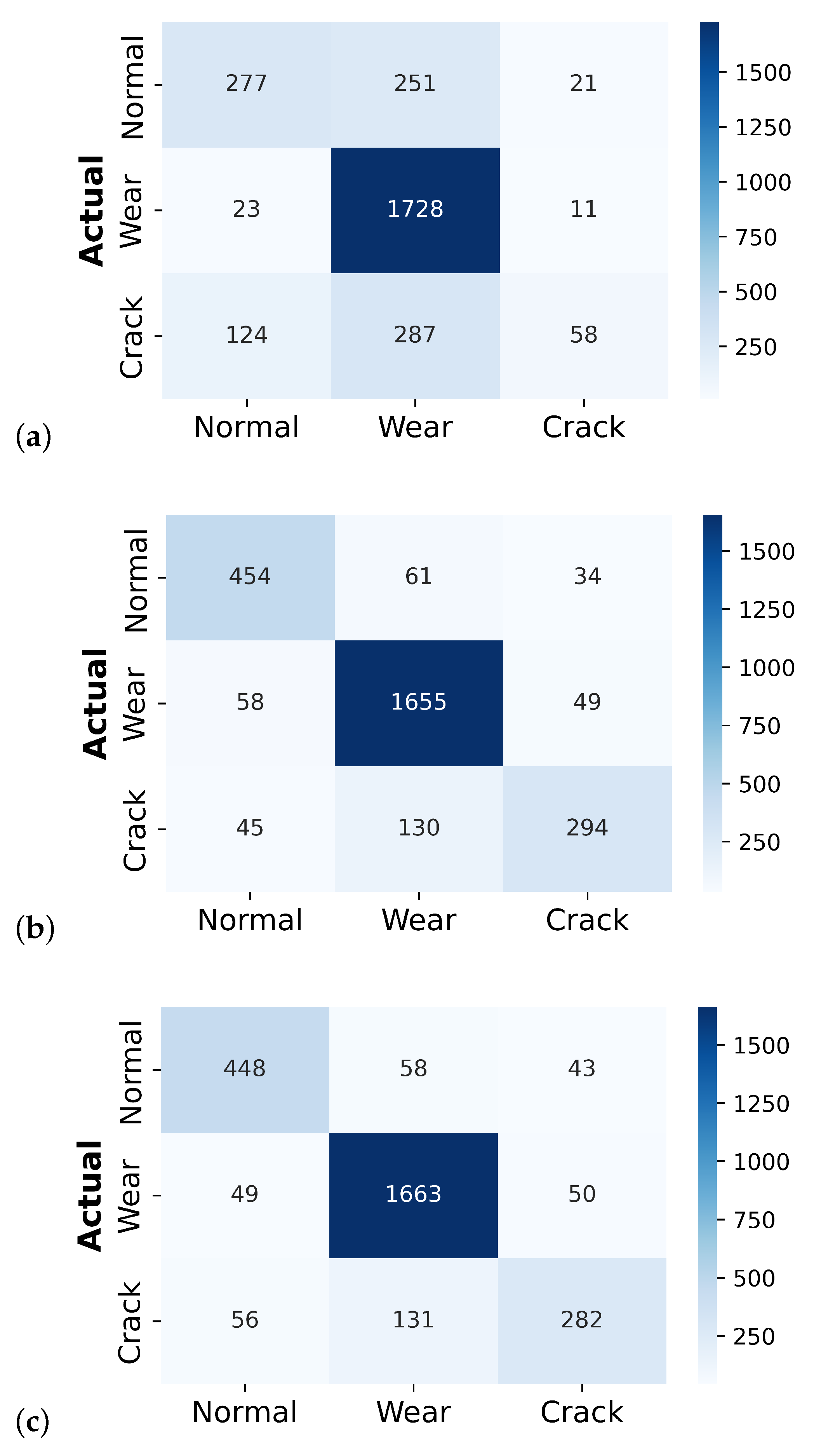
Figure 10 show the confusion matrix plot for the classifier model before and after augmentation, respectively.
Before data augmentation, the classifiers demonstrated a commendable performance, as reflected in their high accuracy, precision, recall, and F1-scores. For instance, the SVM model showed strong performance, particularly in precision and recall for the majority class (wear), although it faced challenges with minority classes such as regular and crack. The SVM results before augmentation were as follows:
Normal: Out of “196 samples”, “121” were correctly predicted as usual, “66” were misclassified as cracks, and only one was misclassified as wear.
Wear: Among “1737 samples”, the model performed exceptionally well, correctly predicting “1736” as wear, with just one misclassified as a crack.
Crack: Out of “159” crack samples, “64” were correctly identified as cracks, but a significant number (91) were misclassified as normal, and four were misclassified as wear.
These results underscore the critical issue of class imbalance, where the model is biased towards the majority class (wear), resulting in a higher number of misclassifications for the minority classes (normal and crack). Addressing this imbalance is crucial for a more balanced and accurate model performance.
After applying GN and SS, the number of data samples increased significantly, introducing more variability into the training set and helping mitigate some of the class imbalance. This increase in data variability, while leading to a decrease in performance metrics such as accuracy, precision, recall, and F1-score, also led to a rise in true label predictions for the augmented data, particularly for the normal and crack classes. This indicates a promising improvement in the model’s ability to recognize these previously underrepresented classes. The SVM results after augmentation were as follows:
Normal: The normal class saw a substantial increase in sample size to “549”, with “277” correctly predicted as normal, though “251” were misclassified as wear and 21 as cracks.
Wear: Out of “1762” wear samples, “1728” were correctly identified, with a slight increase in misclassifications into the normal (23) and crack (11) classes.
Crack: The crack class also benefited from augmentation, increasing to “469” samples. Here, “124” were misclassified as normal, “287” as wear, and “58” correctly identified as cracks.
These results indicate that while augmentation led to a slight decrease in overall performance metrics, the increase in true label predictions for normal and crack classes is significant. The improvement in the model’s ability to detect these classes suggests that data augmentation helped address the data imbalance issue, providing a more diverse training set that allowed the classifiers to generalize better to previously under-represented classes. The augmentation process demonstrates that while traditional metrics like accuracy, precision, and recall might decrease, the true positive rate for minority classes can improve, leading to a more balanced model performance across different classes. This is particularly evident in the confusion matrix results, where the post-augmentation predictions for normal and crack samples increased significantly across all three models. This improvement can be attributed to the augmentation techniques creating more diverse and representative samples, which reduce the model’s bias towards the majority class.
The random forest (RF) results before augmentation were as follows:
Normal: Out of “137” normal samples, “165” were correctly classified, but “59” were misclassified as cracks.
Wear: The RF model performed excellently in the wear class, correctly classifying “1736” out of “1737” samples and misclassifying only one as a crack.
Crack: A total of “120” out of “159” were correctly identified as crack samples, but “39” were incorrectly labeled as normal.
After Augmentation, we had the following results:
Normal: The number of normal samples increased to “549”, with “454” correctly predicted. This represents a significant improvement in the true positive rate for normal samples, which is a key benefit of data augmentation. However, the model now misclassified “61” samples as wear and “34” as cracks, introducing more variability in misclassification.
Wear: Among the “1762” wear samples, “1655” were correctly identified, showing a slight decline from the pre-augmentation performance. A total of 58 were misclassified as normal, and “49” were classified as cracks.
Crack: For the crack samples, the model correctly classified “294” out of “469” samples. However, the increase in misclassifications, particularly into the wear category (130 samples), indicates that while the model’s ability to detect cracks improved, it also became more prone to confusion between similar classes.
The RF model’s performance metrics slightly declined after augmentation, with a noticeable misclassification increase across all classes. However, the model showed a marked improvement in identifying normal samples which were previously underrepresented. The increase in true positives for the normal class suggests that the augmented data provided more diverse examples for the model to learn from, reducing bias towards the majority class (wear). The trade-off here is an increase in the number of misclassified samples, particularly for the crack class. This may indicate that the augmented data introduced new complexities that the RF model struggled to generalize.
The Gradient Boosting (GB) results before augmentation were as follows:
Normal: Out of “196” normal samples, 139 were correctly classified, with “57” misclassified as cracks, which was similar to the RF.
Wear: The GB model performed almost flawlessly for the wear class, correctly classifying “1736” out of “1737” samples, with only one misclassification as a crack.
Crack: Among the crack samples, “122” out of “159” were correctly classified, with 37 misclassified as normal.
After Augmentation, we had the following results:
Normal: The sample size for normal increased significantly, with “448” out of “549” samples correctly identified. The misclassification rates were “58” as wear and “43” as cracks, showing an improvement in identifying normal samples but with similar misclassification patterns as the RF.
Wear: The GB model correctly identified “1663” out of “1762” wear samples, showing a slight decline in accuracy compared to the pre-augmentation results. This decline underscores the trade-offs involved in improving class representation through data augmentation.
Crack: The model correctly classified “282” out of “469” crack samples. However, misclassifications increased, with “56” labeled as normal and “131” as wear, indicating a similar challenge in distinguishing cracks from other classes.
The GB model, like the RF, decreased its overall performance metrics after augmentation but with an improved true positive rate for the normal class. The augmentation led to a better balance in class representation, particularly for normal and crack samples, which were previously underrepresented. However, the model’s ability to accurately distinguish between similar fault types, especially wear and crack, was somewhat compromised. This suggests that while the augmented data helped address the class imbalance, they also introduced additional complexity that the model had difficulty managing, leading to increased misclassifications.
Table 8 presents the performance metrics, including accuracy, precision, recall, and F1-score, before and after data augmentation through GN addition and SS. The data augmentation techniques applied in this study played a significant role in enhancing the performance of the ML models by effectively increasing the diversity of the dataset. This introduction of variability in the input features improved the models’ ability to generalize and recognize previously unseen patterns in the data.
After data augmentation, some models’ accuracy improved, particularly in detecting under-represented classes like “normal” and “crack.” For example, while showing a slight decrease in overall accuracy, the SVM model exhibited a significant improvement in its true positive rates for these minority classes, indicating a better balance in model performance across different conditions. The precision and recall metrics further highlight this improvement. Post-augmentation, the models demonstrated improved recall, especially for minority classes that were previously misclassified. This suggests that the augmented data helped the models become more sensitive to detecting anomalies and normal conditions, which were under-represented in the original dataset.
The F1-score, which harmonizes precision and recall, generally improved or remained stable after augmentation. This suggests that the models maintained a good equilibrium between correctly identifying faults and minimizing false alarms, which is a critical aspect in an industrial setting. In particular, the RF and GB models displayed a more consistent performance improvement after augmentation. Despite a slight trade-off in terms of increased misclassification in some cases, the models’ overall ability to correctly identify faults, particularly in complex and noisy environments, was enhanced.
The augmentation process effectively addressed the class imbalance, providing the models with more diverse training examples. However, introducing more complex variations in the data, such as highly distorted signals or extreme noise levels, likely increased the misclassification rates, particularly in more complex fault types (wear and crack). This highlights the importance of carefully balancing augmentation techniques to ensure that, while class representation is improved, the data remain distinguishable by the models. Applying data augmentation techniques led to a more robust and generalizable set of ML models. Although the traditional performance metrics like accuracy, precision, and recall may have shown minor declines, the true positive rate for the minority classes and overall model robustness were significantly enhanced. This resulted in more reliable fault detection and diagnosis in practical applications, making the models better suited for industrial use.
5.4. LSTMAEGAN Modeling Result
In this study, we employed a comprehensive data pre-processing and augmentation pipeline to enhance the robustness of our diagnostic models for centrifugal pumps. The pump vibration data collected were first normalized using MinMaxScaler and then segmented into sequences of 100 time steps each to preserve temporal patterns. These sequential data were divided into training and testing sets, with 20% reserved for testing. An LSTM-based Autoencoder was implemented to capture the expected behavior of the pump, with its performance evaluated based on the reconstruction error measured as the Mean Squared Error (MSE). A threshold, set at the 95th percentile of the reconstruction error distribution, was used to identify anomalies—those sequences with errors exceeding this threshold. A GAN network was developed to improve anomaly detection further. It consisted of a generator and discriminator trained to produce synthetic sequences resembling the vibration data. This approach introduced additional variability and enhanced the model’s generalization capabilities.
The performance of the anomaly detection model was evaluated using key metrics, yielding high scores—an accuracy of 1.0; a precision of 1.0; a recall of 0.98; and an F1-score of 0.99. The confusion matrix confirmed these results, showing that the model correctly identified most sequences while misclassifying only a small number.
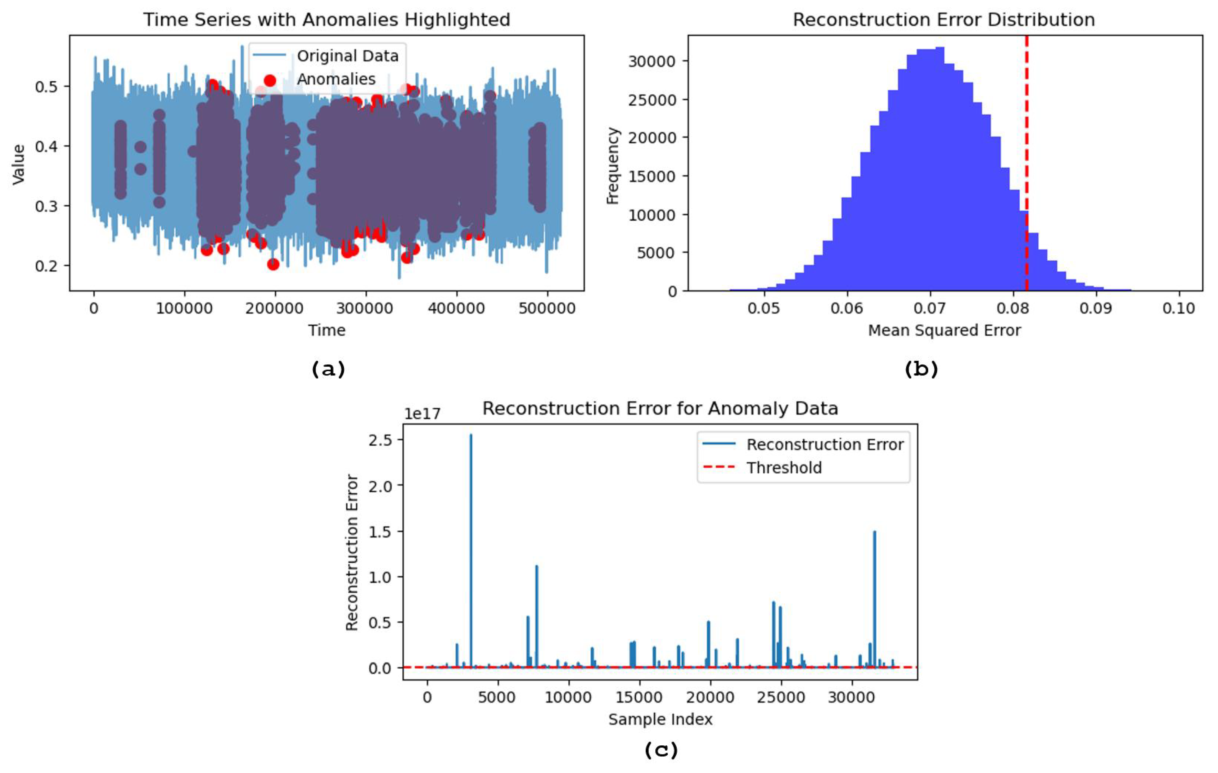
Figure 11 illustrates the further analysis of the model’s performance. The time series plot with highlighted anomalies provides a visual overview, where anomalies—marked by red dots—clustered at specific intervals. This clustering suggests that the system experienced recurrent deviations from its normal operation, which are potentially indicative of underlying faults or operational irregularities. These anomalies may correspond to particular pump cycles or external factors affecting the system.
The reconstruction error distribution, presented in a histogram, resembles a Gaussian curve typical of well-functioning systems. The red dashed line represents the anomaly detection threshold, which has been strategically placed to flag only the most significant deviations. This placement is critical for balancing sensitivity and specificity, ensuring that the model effectively distinguished between normal and abnormal data. A closer examination of the reconstruction errors for the anomaly data reveals spikes above the threshold, indicating instances where the model struggled to reconstruct the original data, leading to significant deviations. The varying magnitude of these spikes implies differences in the nature or severity of the anomalies, which could be crucial for maintenance strategies. This variation allows for prioritizing responses to different types of faults based on their impact or frequency.
Together, these analyses demonstrate the model’s proficiency in detecting subtle and severe anomalies, underscoring its robustness in handling time series data. Integrating data augmentation and advanced modeling techniques, such as the LSTMAEGAN, ensures that the model generalizes well across different fault types, making it a reliable tool for real-world predictive maintenance applications. This capability enhances the reliability and efficiency of industrial systems and provides a promising outlook for the future application of this model in various operational contexts.


