In this section, we describe random walks in a fine-grid network in a one-dimensional space–time prism and the visit probability they induce on the prism. It is convenient to describe such a random walk in a local coordinate system that fits the grid in the prism in which the random walk takes place. In the treatment of the one-dimensional case, we assume that . The case is completely analogous.
4.1. Random Walks in the Future Cone and Their Local Coordinate System
Given a one-dimensional prims , we first describe, for any non-zero natural number ℓ, a finite process which generates a random walk that starts at the anchor point and arrives, after ℓ steps, at the time level of the second anchor point, while remaining within the bottom cone of the prism. For a non-zero natural number ℓ, which denotes the number of steps of the random walk, we call the corresponding step size (or time granularity) of this walk.
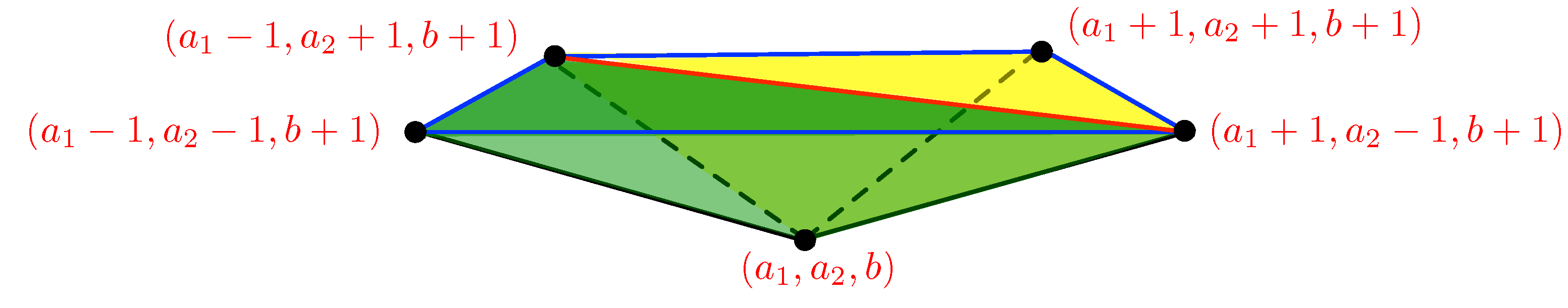
The random walk process of ℓ steps starts at level 0 in the anchor point . The i-th step of its ℓ steps brings the moving object, performing the random walk, from level to level i. At each level of the process, the moving object starts at some previously reached space–time location and makes, randomly (with equal probability ), one of the following two moves in the future cone of the prims :
- (1)
from to ; or
- (2)
from to .
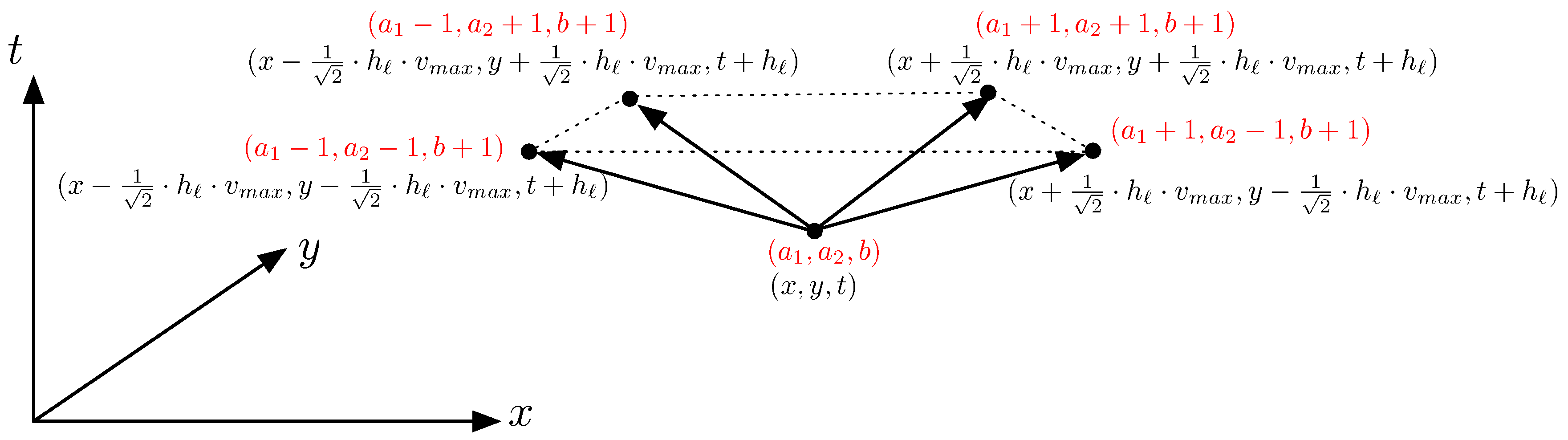
The two possible steps of the random walk process are illustrated in
Figure 2 and they correspond, after the toss of a coin, to moving from
x to the left, respectively to the right, at maximal speed
for a time duration
. In between levels, we assume these random walk steps to follow linear paths at a maximal speed between these points.
The above-described process arrives, after
ℓ steps, at the time level
but it is not guaranteed that it can reach the spatial location
of the second anchor point at that moment. For example, if
,
and
(
Figure 3 can be used as an illustration), then there is no random walk of
steps from the first to the second anchor point. Indeed, a random walk would take steps of size
in time and in distance. If it would take
l steps to the left and
r steps to the right to reach the second anchor point, we would have
and
. However, these equations do not have a solution for
l and
r in the natural numbers. Furthermore, the right rim point of this prism has coordinates
and is also not reachable in five stes or fewer from the first anchor point. On the other hand, if we would take
steps, then the second anchor point can be reached by taking 5 steps to the right (arriving in the right rim point), followed by 3 steps to the left, for example.
The ability of a random walk process to reach the second anchor point and, to a lesser extent, the two rim points, is a desirable property, however. The following proposition shows how an appropriate number of levels (and corresponding step size) can be chosen to achieve this. This property only depends on the assumption that and the coordinates of the anchor points are rational numbers. Since the anchor points and are the result of measurements (by GPS, for example), this is not unreasonable to assume. For practical purposes, can also be assumed to be a rational number. The proof of this property contains a method to determine a “minimal” number of levels.
Proposition 1. For rational and anchor points and with rational coordinates, we can determine, from these rational numbers, a “minimal” number of levels such that a random walk in the bottom cone of the prism can reach the second anchor point after steps and such that also the two rim points can be visited by random walks of at most steps.
Proof. We assume that and the coordinates of the anchor points and are rational numbers. We would like the random walk process, starting in the first anchor point, to be able to reach the second anchor point and the two rim points of the prism . Let be a number of levels (with corresponding step size ) that we are looking for. Let and be the number of steps needed to reach the right rim point and the left rim point in a straight motion, respectively. Let be the “displacement” of the second anchor point, as given by (1), below.
Being able to reach the second anchor point and the two rim points after a finite number of steps in some random walk process corresponds to the existence of natural numbers
and
and an integer
such that the following six equalities hold:
Lines (1–2) concern the second anchor point (and (2) is trivially satisfied); lines (3–4) concern the left rim point; and lines (5–6) concern the right rim point. For the left and right rim point, it is important to remark that they can only be reached in one way, namely by moving at maximal speed to the left or the right, respectively, away from .
From (1), we obtain . We remark that we assume that , which corresponds to the prism being non-empty. We write the positive rational number as a division free fraction and take and . Therefore, we have or .
From (3–4), it easily follows that we can take , which is a natural number. From (5–6), it easily follows that we can take , which is also a natural number.
So, it follows that by writing as a division free fraction we can find the minimal number of levels that a random walk can take to fit the prism boundaries. ☐
The proof of the above proposition gives a “minimum” number of levels
and an associated “displacement”
of the second anchor point (corresponding to a shift in the spatial dimension). Obviously, any multiple of the values
and
can also be used for a suitable random walk in the prism. From now on we will work with a number of levels
ℓ and a displacement
d that are multiples of
and
, that is,
and
for some
. Thus, Proposition 1 gives rise to a family (parameterized by
ℓ) of fine-grid networks (in the terminology of Burns [
30]), on which the the random walk can take place.
Based on the above observations, we can define a local (discrete) grid network and corresponding coordinate system on the bottom cone
(and thus on the prism
), which determine the space–time points in which steps in a random walk from
to
start or end. The local coordinate system assigns the local coordinates
to the first anchor point
and the numbering of further space–time points in a random walk follows the rules: if a grid point with Cartesian coordinates
has local coordinates
, then
and
have local coorinates
and
, respectively. Local coordinates are illustrated in
Figure 2, in red. If the second anchor point
has local coordinates
, we speak about a
-grid (or
ℓ-grid, since
d can be derived from
ℓ) on the prism, when we limit the grid in the future cone to the prism
.
This means that, given some local coordinates in a -grid, the corresponding Cartesian coordinates are . We refer to the first coordinate of the local coordinate system as the displacement a and to the second coordinate as the level b. It is important to remark that in a -grid the local coordinates are always such that is even. The value a varies from to b in steps of 2 at level b in the bottom cone of the prism. If we call the value the rank of a (at level b), for grid points , we can equivalently say that the rank varies from 0 to b in steps of 1 at level b.
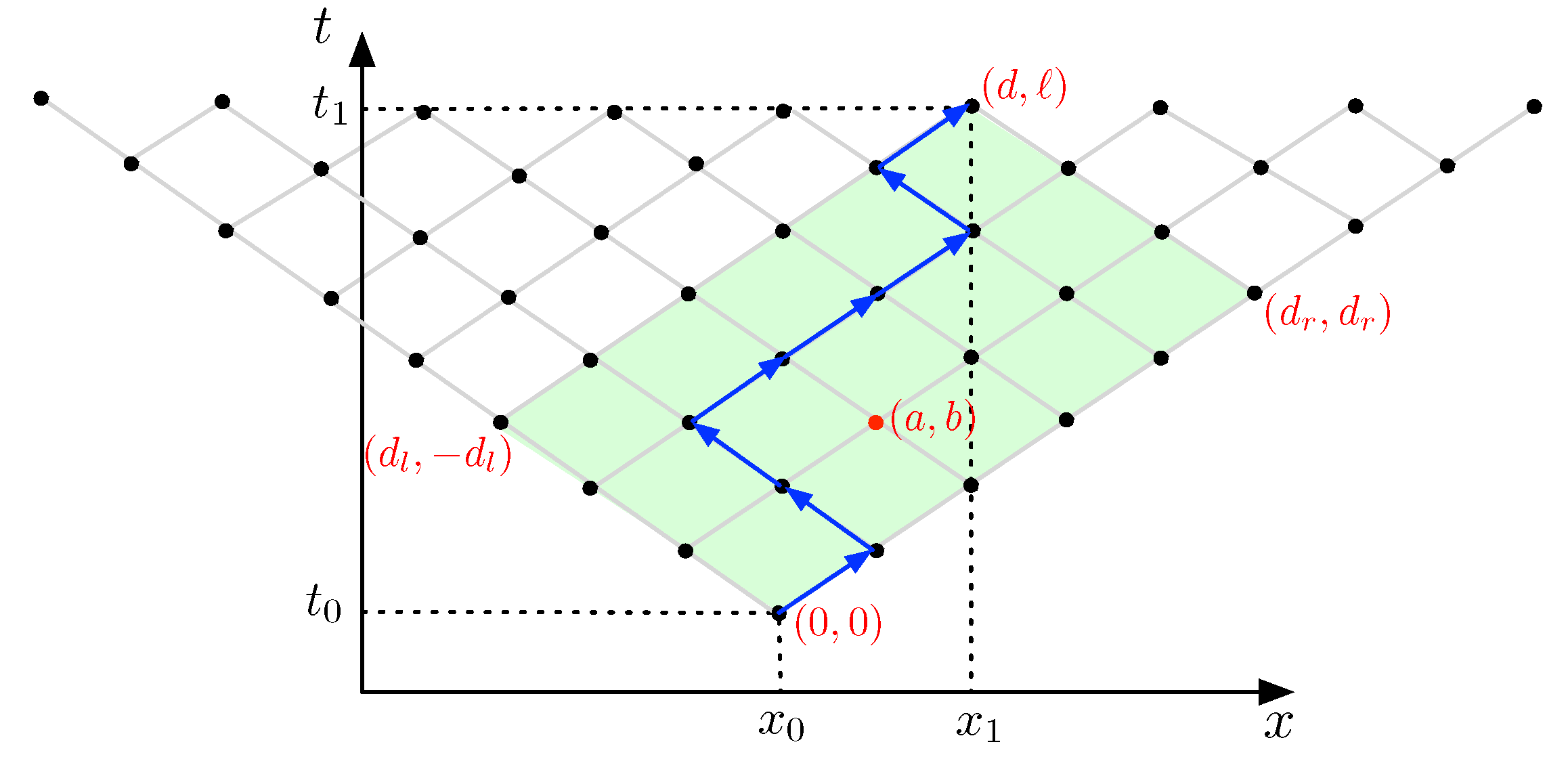
The grid and local coordinate system are illustrated in
Figure 3 with an example in which the number of levels
,
,
and
. The anchor points
and
have local coordinates
and
, respectively. The rim points
and
have local coordinates
and
, respectively.
Figure 3 also shows an example of a random walk path from the first to the second anchor point where the coin tosses produced the path given by the sequence right-left-left-right-right-right-left-right.
We conclude this section by remarking that a random walk from the first to the second anchor point of the prism
can be finitely represented, in the local coordinate system, as a sequence
of grid points, with
. When a random walk, after
ℓ steps, arrives at the second anchor point
, we can then observe that the space–time path resulting from such a random walk (after linear interpolation between the consecutive visited grid points) respects the maximal velocity constraint
and is therefore a trajectory within the prism
that connects the anchor points. For a precise definition of trajectories in a prism and their velocity, we refer to [
51] (with speed bound
).
4.2. Random Walk Visit Probability in Points of a Fine-Grid Network
In this section, the goal is to establish the visit probability in a grid point with local coordinates
in a
-grid on a one-dimensional prism
. The visit probability of such a grid point is the number of random walks (following the principles, described in
Section 4.1) that start at the first anchor point of the prism
, that pass through the grid point
, and finish in the second anchor point divided by the total number of random walks from the first to the second anchor point.
We denote the number of random walks that start in the first anchor point and arrive at the grid point with local coordinates by . At level 0, we agree that there is one random walk (of length 0) that arrives at the first anchor point. At level 1, each of the two grid points has one path arriving there. These correspond to the two choices (left or right) that can be made in the first anchor point. This means that we have and .
For each point, with local coordinates
, at a higher level, a random walk arriving there arrives either from
or from
, provided that the latter points are in the bottom cone. Therefore, we have
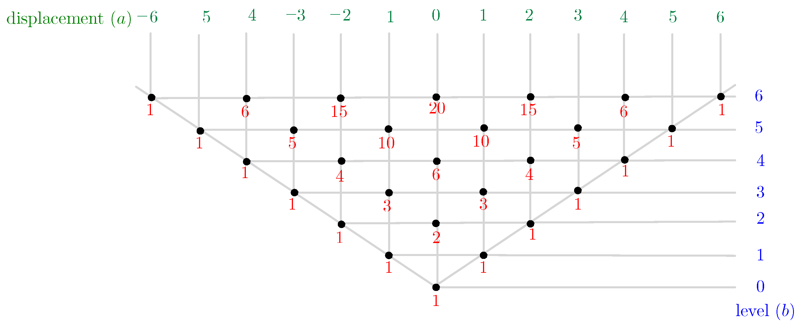
if we consider the terms in this sum that correspond to points outside the bottom cone to be 0. Following the above observations, we recognise that the values
can be read from the well-known binomial triangle (or Pascal’s triangle), since
and we obtain
for
integers with
,
and
even. In terms of generating functions, we can say that
is the coefficient of
in the expansion of the (rational) polynomial
(the proof is straightforward). In this polynomial,
x expresses a move to the right and
corresponds to a move to the left.
Figure 4 gives an illustration of the values
for level 0 to level 6 on a random walk grid.
After having established the number of random walks that arrive at , we need to establish the number of continuations of such walks from to the second anchor point . Hereto, it is sufficient to determine the number of “time-reversed” random walks in the future cone that start from the second anchor point and that, moving back in time, arrive in . We denote the number of such downward random walks by . Each such downward random walk, when time-reversed is an upward random walk from the point to the second anchor point .
More formally, we can use the mapping
(in Cartesian coordinates) or the mapping
(in local coordinates) to map the top cone of the prism
onto its bottom cone. When we then apply the earlier method for the bottom cone, we easily verify that
. The number of paths that come down from the second anchor point and that pass through
in the top cone therefore is
Each random walk in the bottom cone from the first anchor point that arrives at
can then be combined with such a time-reversed random walk from
to the second anchor point to form a random walk going from the first to the second anchor point of the prism, passing through
. The total number of random walks in the prism from the first anchor point to the second anchor point, passing through
, therefore is the product of
and
and we denote this product by
. Therefore, we have
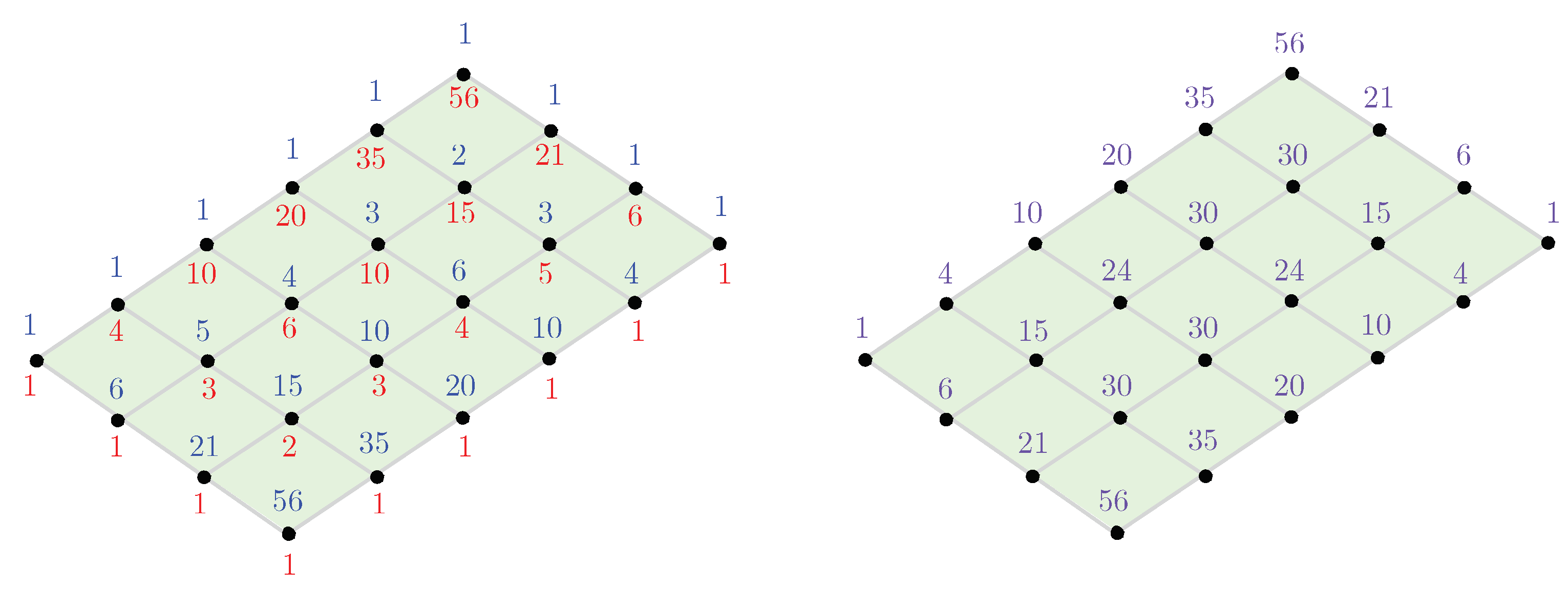
The values of
,
and
are illustrated in
Figure 5.
We remark that the total number of random walk paths in the prism
can be read at one of the anchor points, meaning that it is
. In the example of
Figure 5, the total number of random walks between the anchor points is
.
Now, we are ready to give a definition of “visit probability”, relative to a chosen number of grid levels ℓ. This definition says that the visit probability of a grid point is the fraction of random walk paths in the prism passing through it.
Definition 2. Let be a prism and let ℓ be a suitable number of levels for this prism. Let be a point in the ℓ-grid on the prism, given in local coordinates. We define the (one-dimensional) visit probability of (relative to the number of levels ℓ), denoted , to be
From this definition and the above observations, we immediately obtain the following result.
Theorem 1. For a grid point of a -grid on a prism , we have Using basic properties of binomial coefficients, we can rewrite this in another useful form as
When we fix a level b and sum the visit probability over all a values at level b, we expect to obtain 1. This reflects the fact that any random walk from anchor to anchor passes the time slice corresponding to level b with absolute certainty. The following property verifies this fact.
Proposition 2. For any level b, we have
Proof. The rank of
a at level
b varies from 0 to
b. Some of these ranks correspond to points
outside the prism, in which case
. From
, we obtain
where
r represents the rank. This sum equals 1, since
by the well-known Vandermonde’s identity, which can be easliy derived by looking at the coefficient of
in the expansions of both sides in the equality
, using the binomial theorem. ☐
4.3. Random Walk Visit Probability on the Complete Prism
The visit probability, based on the random walk model, as defined in Definition 2, is specified on the grid points of a -grid only. In this section, we discuss how it can be defined on the complete prism. We first discuss the type of distribution associated with this visit probability and the effect of increasing the number of levels of the grid.
4.3.1. The Distribution Corresponding to the Visit Probability
Here, we discuss the type of probability distribution that the visit probability, described by Theorem 1, gives rise to. The first fraction in
in Theorem 1, shows that, for each level
b, the expression for
corresponds to a hypergeometric distribution in the rank
[
52,
53]. In fact, if we consider the cumulative density function
for our situation, we get
The functions
and
are so-called hypergeometric functions and we may conclude that we have a hypergeometric distribution [
54].
Distributions and also hypergeometric distributions are typically characterized by a number of quantities, such as the mean; the variance; the skewness; and the excess kurtosis [
52,
53].
In our setting the mean is . It is easily verified that the point at level b, that represents the mean, has a rank that places it on the diagonal of the prism (given by , in the local -coordinates).
The variance is . This variance is tending towards zero towards the anchor points of the prism and reaches its maximum at the level (remark that according to Proposition 1 a suitable ℓ is always even).
The skewness is . The skewness is negative for , which means that the distribution has a tail (or is stretched) to the left. This is explained by the fact that the left side of the prism, for , is further away from the diagonal that its right side. It is zero for , which means we have a normal distribution at that level. The skewness is positive for , which means that the distribution has a tail to the right. At the levels and the skewness is infinite, which indicates the peak at the unique value at these levels. The the excess kurtosis describes how flat or peaky the distribution curve is. In our case, it is a long and complicated expression that we omit here. We only mention that it is negative, which indicates a rather “flat” distribution curve.
4.3.2. The Effect of Refining the Fine-Grid Network
One way to move from a visit probability that is only defined on grid points to one that is defined on the whole prism is to increase the number of levels ℓ, thus approximating each point in the prism eventually by a grid point. In this paragraph, we investigate how the expression for the visit probability in Definition 2 depends on the number of levels ℓ. As an increase in the number of levels, we consider doubling the number of levels and we investigate the effect thereof.
We start with an
-grid, as described in
Section 4.1, and than refine this grid, by for instance iteratively doubling the number of levels, resulting in a
-grid, with
i a non-zero natural number. This way, we obtain finer and finer grids and an arbitrary point
in the prism
can be approximated arbitrarily close. A downside of doubling the number of levels is that the visit probability decreases (and ultimately goes to zero), as the following property shows. This is due to the fact that, when doubling the number of levels, the number of possible paths roughly squares. First, we remark that when the number of levels is doubled, a spatio-temporal point with local coordinates
in a
-grid, will have
as local coordinatesa in a
-grid. In particular, the second anchor point which has local coordinates
in the original grid will have local coordinates
after doubling the number of levels.
Proposition 3. For and b as before, we have .
The proof of this property is a direct consequence of the well-known estimate
from which it follows that
, and thus
, provided that
. For non-extreme visit probabilities, we thus obtain that the sequence
converges (by the Weierstrass–Bolzano theorem) to 0, expressing that individual points in finer and finer grids have a visit probability that tends to 0.
This last observation is not surprising. In an infinite set of space–time points, as a prism is, it is to be expected that individual elements have a probability 0. The usual approach to deal with this is to use probability density functions and cumulative density functions, which would allow us to determine the visit probability of a small area around an arbitrary point
in a prism
, for instance. Such an area is usually an
-box of type
. To obtain an exact solution for our case, we can turn to Pearson distributions [
55,
56], which are the continuous analog of hypergeometric distributions. In our case, we observe that, since the excess kurtosis is negative, the Pearson distribution would be of type 2. Due to the complexity of these Pearson distributions, we present a more practically usable approach in
Section 4.3.3.
4.3.3. A Definition of Visit Probability on a One-Dimensional Prism
In this section, we give a practically usable definition of visit probability for all points in a one-dimensional prism. For our definition, we assume that a number of levels ℓ in a grid have been chosen. This number of levels ℓ and the corresponding step size may depend on the application at hand. When the application concerns moving objects that are pedestrians we may want to set to one meter, whereas in the context of moving cars, it may be taken to be larger.
When a number of levels
ℓ is fixed, Definition 2 gives us values for the visit probability in grid points on the
ℓ-grid on the prism. To determine a value for the visit probability in non-grid points, we use linear interpolation, based on barycentric coordinates in which we use the three closest grid points. This approach gives a more continuous result, as opposed to the voxel-based approach of, for example, References [
31,
32] and of the random-walk part of [
24,
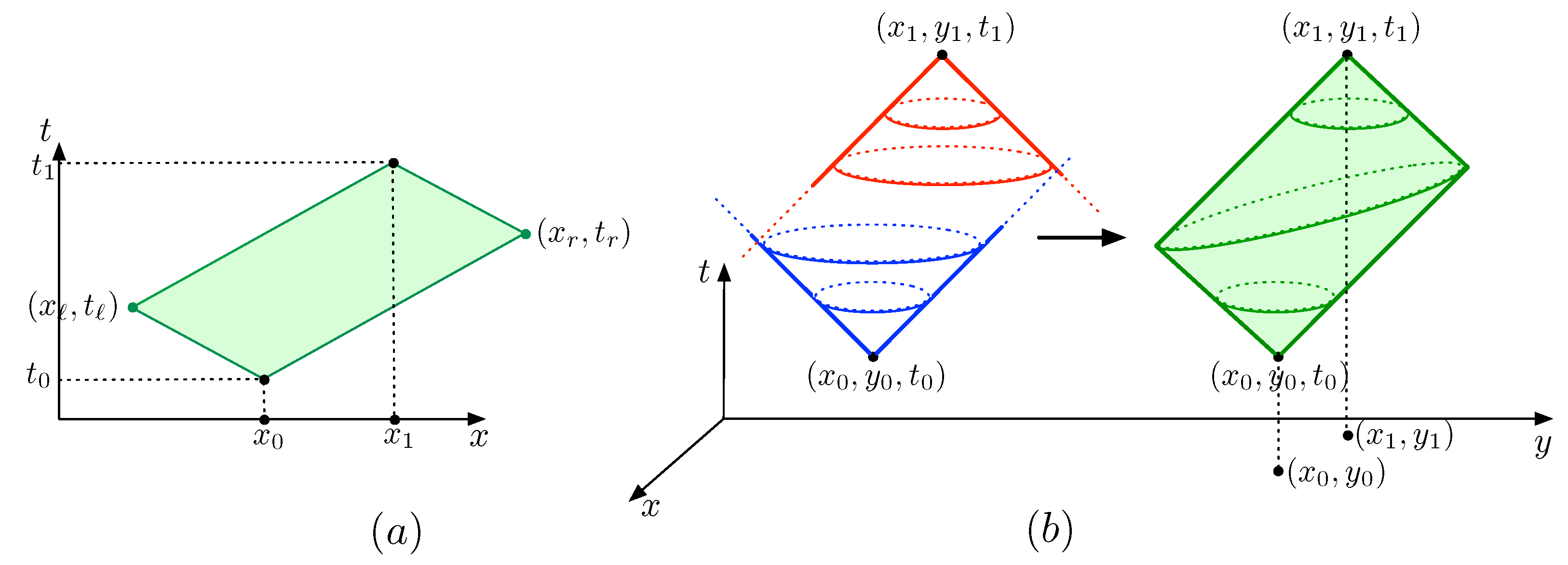
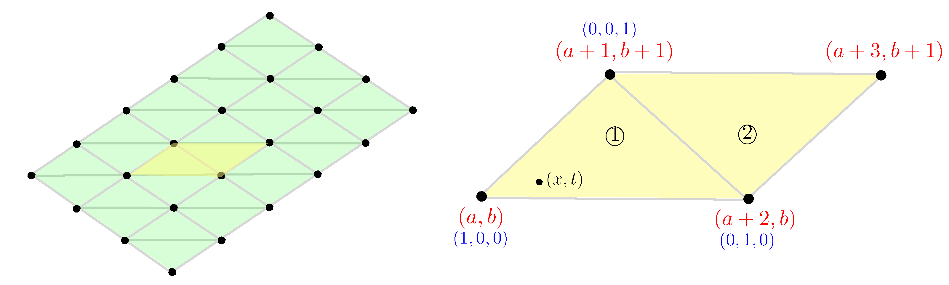
26]. Hereto, we partition the grid points into triangles by adding horizontal lines to the grid lines that are already shown in
Figure 3. This partition is illustrated in the left part of
Figure 6, where also the two types of triangles occurring herein are shown (indicated as ① and ②). We develop the definition of the visit probability of a point with Cartesian coordinates
in a type ① in full and remark that for type ② triangles the development is completely analogous. A type ① triangle has corner points with local coordinates
,
and
. If we give these corner points barycentric coordinates
,
and
, respectively, then, taking into account that the Cartesian coordinates of a grid point with local coordinates
is
(see
Section 4.1), we have barycentric coordinates
for the point
if
with
and
.
We can easily derive that , and .
Similarly, in a type ② triangle, when we give the grid points with local coordinates , and barycentric coordinates , and , respectively, we obtain barycentric coordinates for a point with the values , and .
Based on these barycentric weights (respectively ) of a point we give the following definition of the visit probability in .
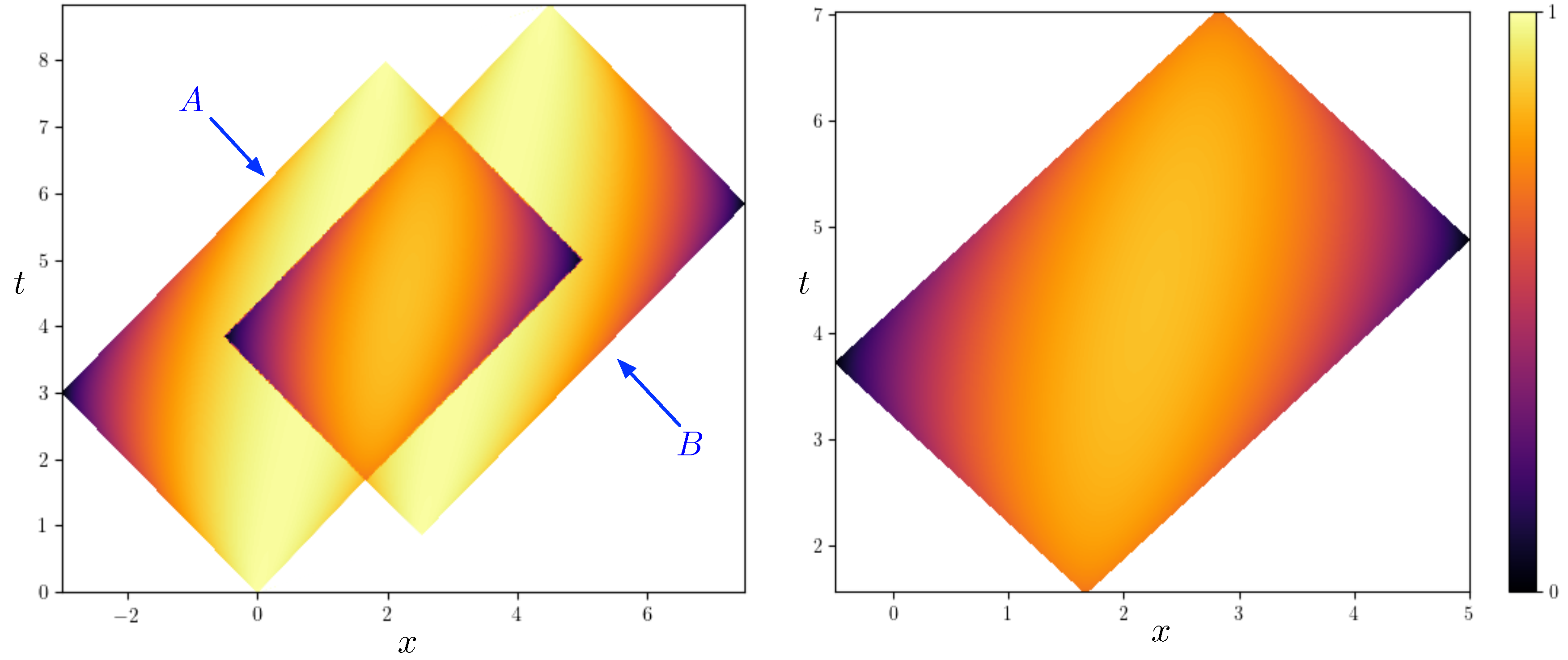
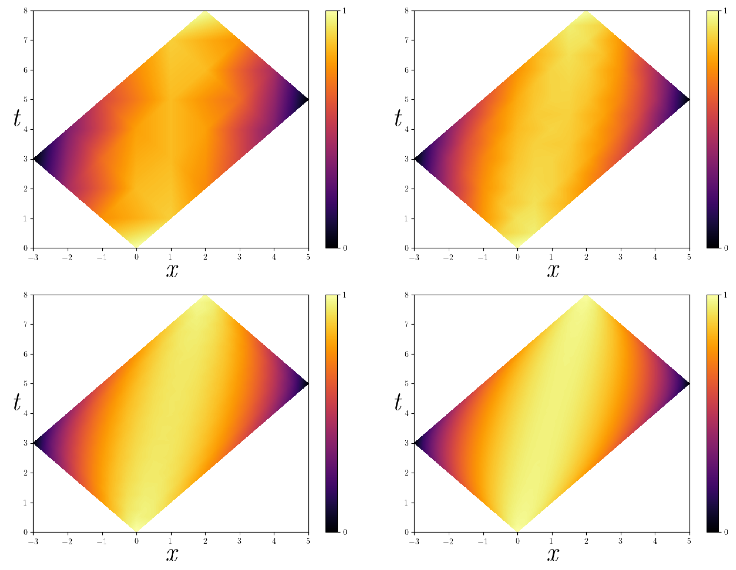
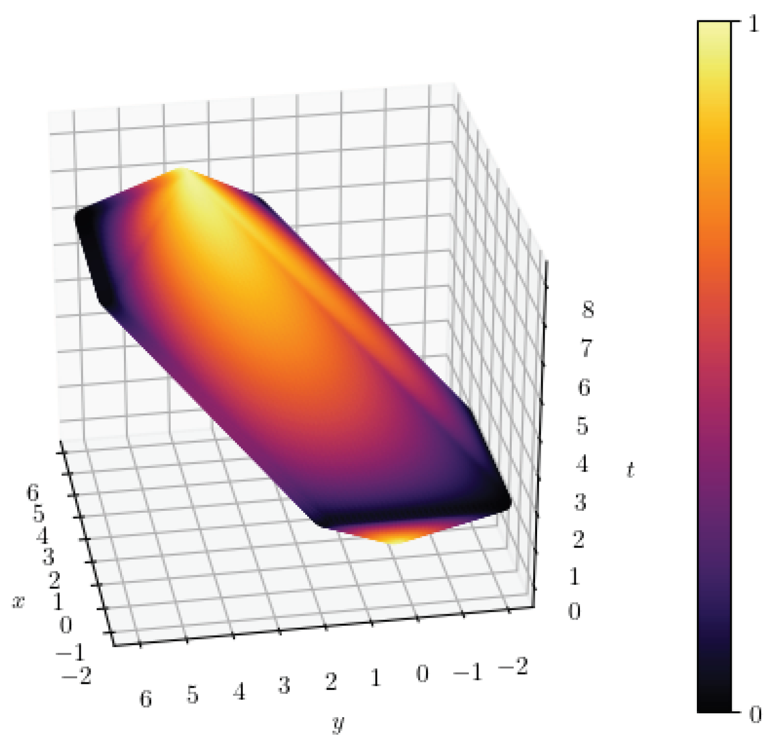
Definition 3. Let be a prism and let ℓ be a suitable number of levels for this prism. If is a point in a type ① triangle, as shown in Figure 6, then we define to be Let be a point in a type ② triangle, as shown in Figure 6. Then we define to be □ Figure 7 shows the barycentric-based visit probability for the prism of
Figure 3, where we take the number of levels
ℓ to be respectively 8, 16, 32 and 64. These illustrations show that the areas around the anchor points have a high probability of being visited, while the areas around the rim points are assigned a very low probability. In general, the diagonal of the prism shows the highest visit probability.

