Earth Observation and GIS-Based Analysis for Landslide Susceptibility and Risk Assessment

 ,
, 
 and
and 
Abstract
1. Introduction
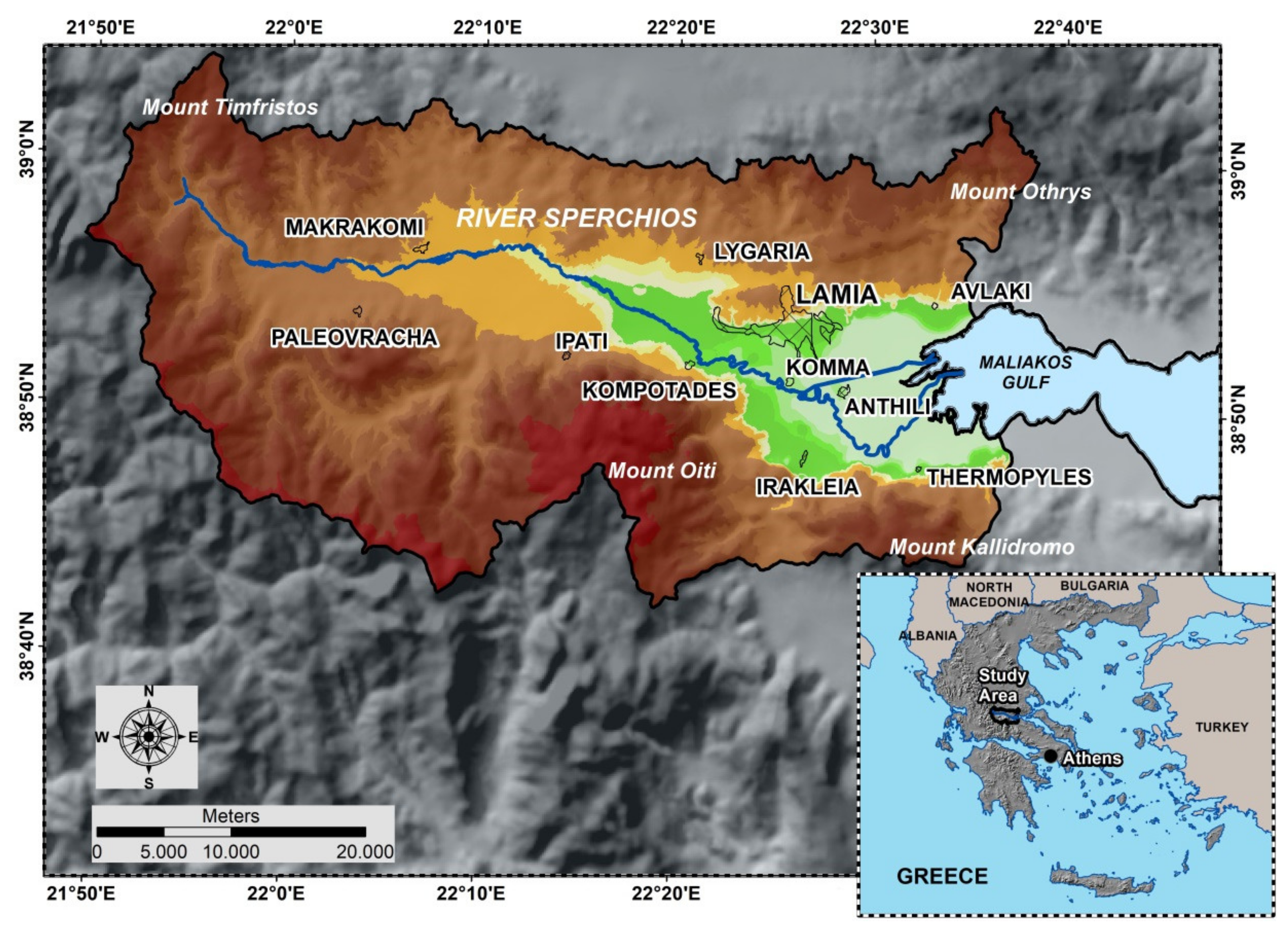
2. Study Area
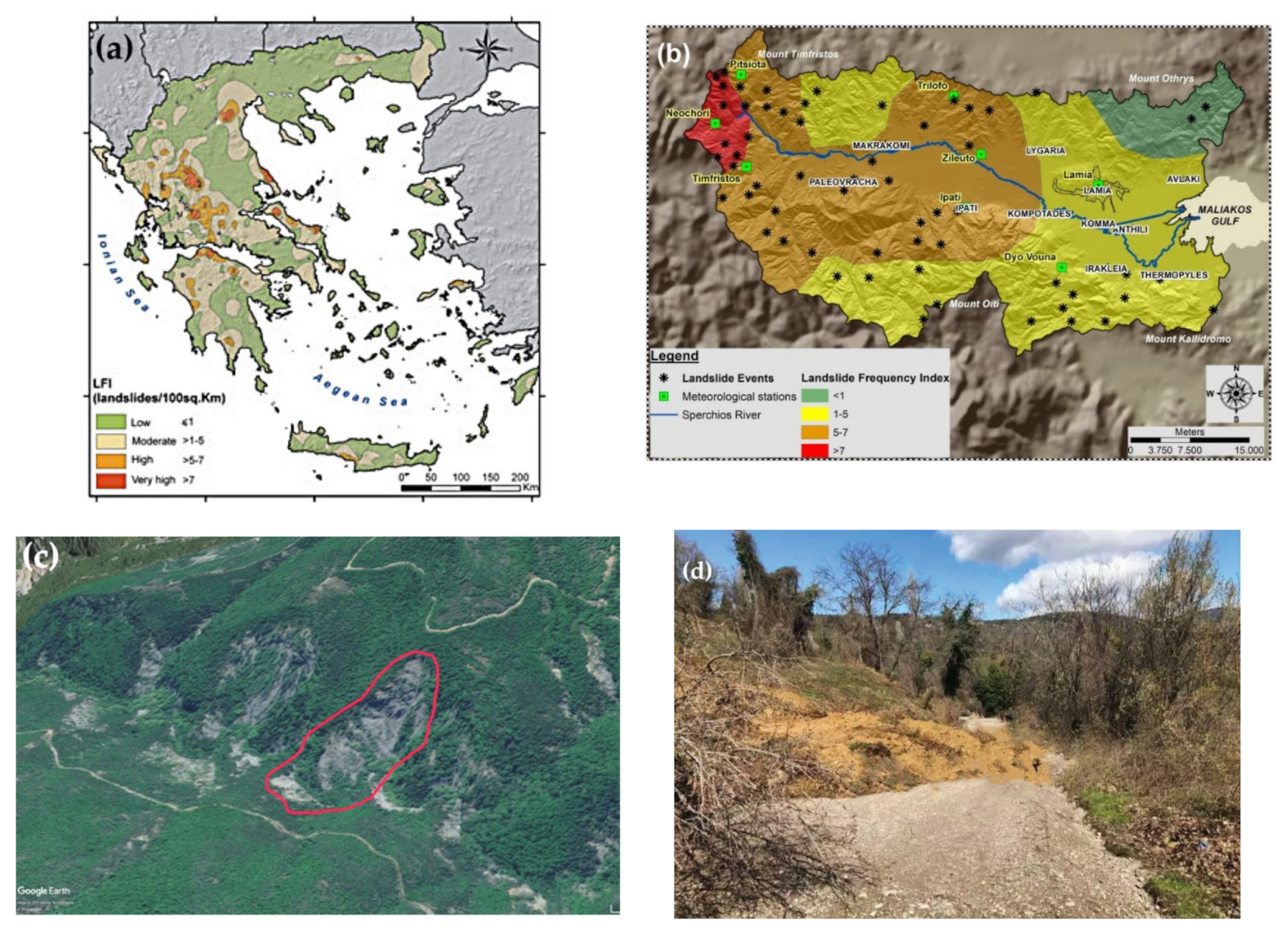
2.1. Landslides
2.2. Inventory Map
3. Materials and Methods
3.1. Dataset
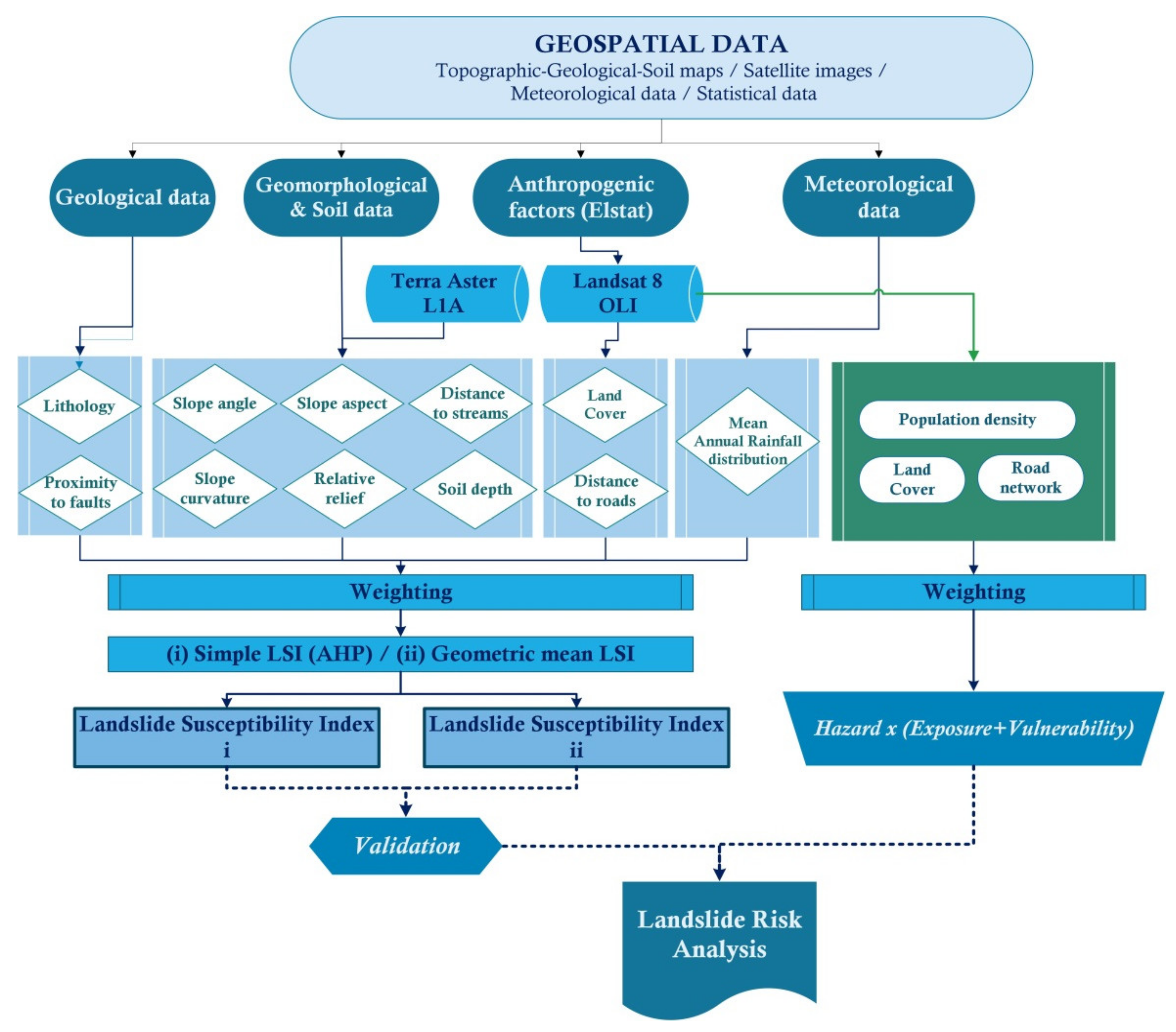
3.2. Methodology
3.2.1. Digital Elevation Model from ASTER Data
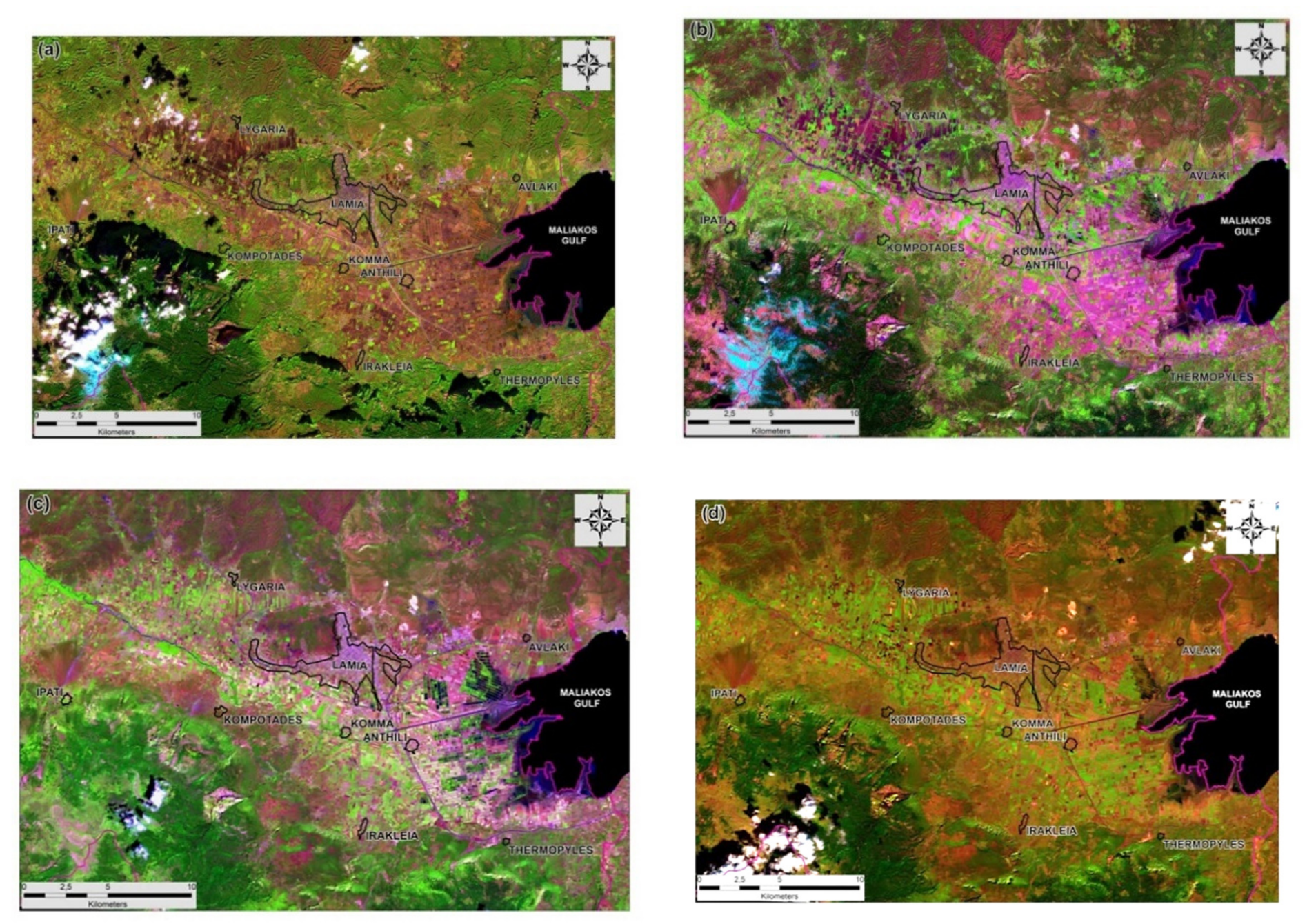
3.2.2. Land Cover Classification from Sentinel Data
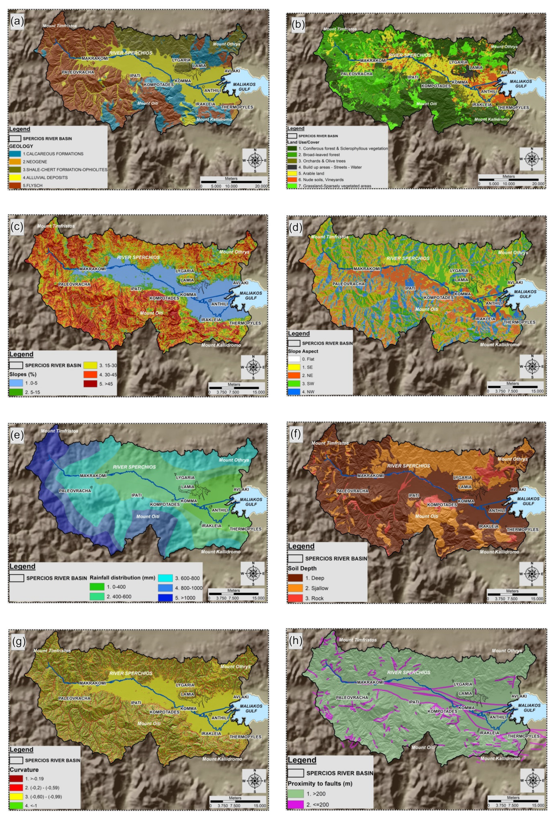
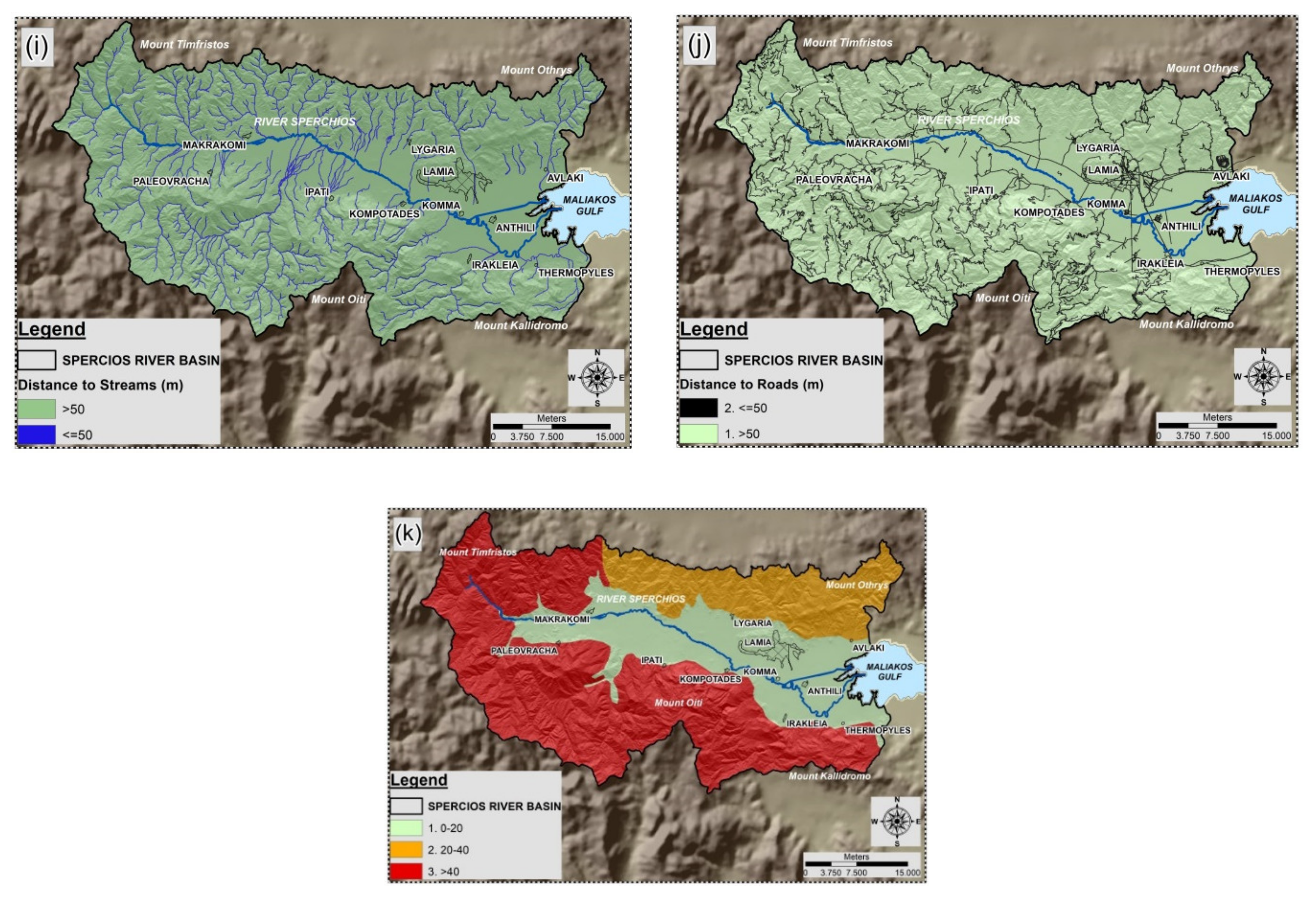
3.2.3. Data Layers Formation
3.2.4. Analytic Hierarchy Process
3.2.5. Weighting of Parameters—Landslide Susceptibility Index
3.2.6. Validation
3.2.7. Landslide Risk Analysis
4. Results and Discussion
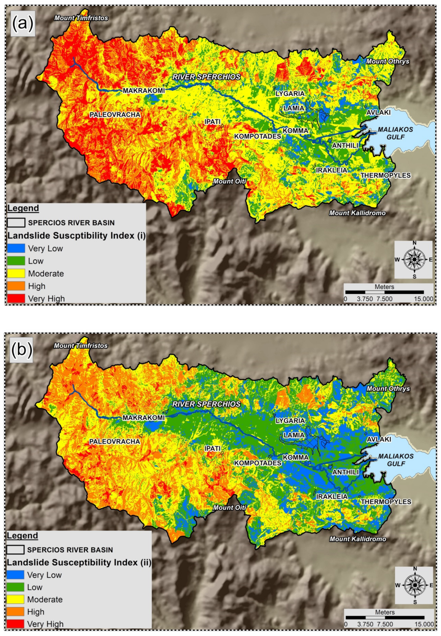
4.1. Landslide Susceptibility Indices
4.2. Accuracy Assessment
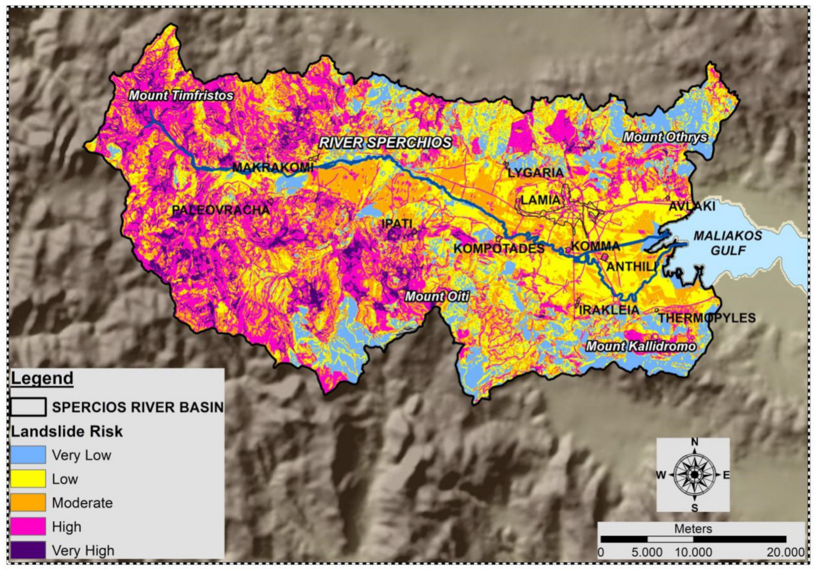
4.3. Landslide Risk
4.4. Discussion
5. Conclusions
Author Contributions
Funding
Acknowledgments
Conflicts of Interest
References
- Cruden, D.M. A simple definition of a landslide. Bull. Int. Assoc. Eng. Geol. Bull. l’Assoc. Int. Géol. l’Ing. 1991, 43, 27–29. [Google Scholar] [CrossRef]
- Yalcin, A.; Reis, S.; Aydinoglu, A.C.; Yomralioglu, T. A GIS-based comparative study of frequency ratio, analytical hierarchy process, bivariate statistics and logistics regression methods for landslide susceptibility mapping in Trabzon, NE Turkey. Catena 2011, 85, 274–287. [Google Scholar] [CrossRef]
- Wang, J.; Peng, X. GIS-based landslide hazard zonation model and its application. Procedia Earth Planet. Sci. 2009, 1, 1198–1204. [Google Scholar] [CrossRef][Green Version]
- Martha, T.R.; Kerle, N.; Jetten, V.; van Westen, C.J.; Kumar, K.V. Characterising spectral, spatial and morphometric properties of landslides for semi-automatic detection using object-oriented methods. Geomorphology 2010, 116, 24–36. [Google Scholar] [CrossRef]
- Rozos, D.; Bathrellos, G.D.; Skillodimou, H.D. Comparison of the implementation of rock engineering system and analytic hierarchy process methods, upon landslide susceptibility mapping, using GIS: A case study from the Eastern Achaia County of Peloponnesus, GREECE. Environ. Earth Sci. 2011, 63, 49–63. [Google Scholar] [CrossRef]
- Chen, W.; Pourghasemi, H.R.; Naghibi, S.A. A comparative study of landslide susceptibility maps produced using support vector machine with different kernel functions and entropy data mining models in China. Bull. Eng. Geol. Environ. 2018, 77, 647–664. [Google Scholar] [CrossRef]
- Achour, Y.; Boumezbeur, A.; Hadji, R.; Chouabbi, A.; Cavaleiro, V.; Bendaoud, E.A. Landslide susceptibility mapping using analytic hierarchy process and information value methods along a highway road section in Constantine, Algeria. Arab. J. Geosci. 2017, 10, 1–16. [Google Scholar] [CrossRef]
- Guzzetti, F.; Carrara, A.; Cardinali, M.; Reichenbach, P. Landslide hazard evaluation: A review of current techniques and their application in a multi-scale study, Central Italy. Geomorphology 1999, 31, 181–216. [Google Scholar] [CrossRef]
- Zhong, C.; Liu, Y.; Gao, P.; Chen, W.; Li, H.; Hou, Y.; Nuremanguli, T.; Ma, H. Landslide mapping with remote sensing: Challenges and opportunities. Int. J. Remote Sens. 2020, 41, 1555–1581. [Google Scholar] [CrossRef]
- Van Westen, C.J.; Rengers, N.; Soeters, R. Use of geomorphological information in indirect landslide susceptibility assessment. Nat. Hazards 2003, 30, 399–419. [Google Scholar] [CrossRef]
- Psomiadis, E.; Papazachariou, A.; Soulis, K.X.; Alexiou, D.S.; Charalampopoulos, I. Landslide mapping and susceptibility assessment using geospatial analysis and earth observation data. Land 2020, 9, 133. [Google Scholar] [CrossRef]
- Kouli, M.; Loupasakis, C.; Soupios, P.; Vallianatos, F. Landslide hazard zonation in high risk areas of Rethymno Prefecture, Crete Island, Greece. Nat. Hazards 2010, 52, 599–621. [Google Scholar] [CrossRef]
- Ladas, I.; Fountoulis, I.; Mariolakos, I. Using GIS & Multicriteria Decision analysis in landslide susceptibility mapping—A case study in Messinia prefecture area (SW Peloponnesus, Greece). Bull. Geol. Soc. Greece 2007, 40, 1973. [Google Scholar] [CrossRef]
- Skilodimou, H.; Bathrellos, G.; Koskeridou, E.; Soukis, K.; Rozos, D. Physical and Anthropogenic Factors Related to Landslide Activity in the Northern Peloponnese, Greece. Land 2018, 7, 85. [Google Scholar] [CrossRef]
- Serey, A.; Piñero-Feliciangeli, L.; Sepúlveda, S.A.; Poblete, F.; Petley, D.N.; Murphy, W. Landslides induced by the 2010 Chile megathrust earthquake: A comprehensive inventory and correlations with geological and seismic factors. Landslides 2019, 16, 1153–1165. [Google Scholar] [CrossRef]
- Chunga, K.; Livio, F.A.; Martillo, C.; Lara-Saavedra, H.; Ferrario, M.F.; Zevallos, I.; Michetti, A.M. Landslides Triggered by the 2016 Mw 7.8 Pedernales, Ecuador Earthquake: Correlations with ESI-07 Intensity, Lithology, Slope and PGA-h. Geosciences 2019, 9, 371. [Google Scholar] [CrossRef]
- Ferrario, M.F. Landslides triggered by multiple earthquakes: Insights from the 2018 Lombok (Indonesia) events. Nat. Hazards 2019, 98, 575–592. [Google Scholar] [CrossRef]
- Guinau, M.; Vilajosana, I.; Vilaplana, J.M. GIS-based debris flow source and runout susceptibility assessment from DEM data? A case study in NW Nicaragua. Nat. Hazards Earth Syst. Sci. 2007, 7, 703–716. [Google Scholar] [CrossRef]
- Sabatakakis, N.; Koukis, G.; Vassiliades, E.; Lainas, S. Landslide susceptibility zonation in Greece. Nat. Hazards 2013, 65, 523–543. [Google Scholar] [CrossRef]
- Hervás, J.; Montanarella, L. Main issues on landslide mapping harmonization in EU member states in the framework of European Commission soil policy. In Guidelines for Mapping Areas at Risk of Landslides in Europe; Hervás, J., Ed.; EUR 23093 EN; Office for Official Publications of the European Communities: Luxembourg, 2007; pp. 7–10. [Google Scholar]
- Fall, M.; Azzam, R.; Noubactep, C. A multi-method approach to study the stability of natural slopes and landslide susceptibility mapping. Eng. Geol. 2006, 82, 241–263. [Google Scholar] [CrossRef]
- Carrara, A.; Crosta, G.; Frattini, P. Geomorphological and historical data in assessing landslide hazard. Earth Surf. Process. Landf. 2003, 28, 1125–1142. [Google Scholar] [CrossRef]
- Hervás, J.; Bobrowsky, P. Mapping: Inventories, susceptibility, hazard and risk. In Landslides—Disaster Risk Reduction; Sassa, K., Canuti, P., Eds.; Springer Science and Business Media: Berlin/Heidelberg, Germany, 2009; pp. 321–349. [Google Scholar]
- Ayalew, L.; Yamagishi, H.; Marui, H.; Kanno, T. Landslides in Sado Island of Japan: Part II. GIS-based susceptibility mapping with comparisons of results from two methods and verifications. Eng. Geol. 2005, 81, 432–445. [Google Scholar] [CrossRef]
- Carrara, A.; Guzzetti, F.; Cardinali, M.; Reichenbach, P. Use of GIS technology in the prediction and monitoring of landslide hazard. Nat. Hazards 1999, 20, 117–135. [Google Scholar] [CrossRef]
- United Nations—SPIDER Knowledge Portal. Disaster Risk Management. Available online: http://www.un-spider.org/risks-and-disasters/disaster-risk-management (accessed on 7 July 2020).
- Kayastha, P.; Dhital, M.R.; De Smedt, F. Application of the analytical hierarchy process (AHP) for landslide susceptibility mapping: A case study from the Tinau watershed, west Nepal. Comput. Geosci. 2013, 52, 398–408. [Google Scholar] [CrossRef]
- Foumelis, M.; Lekkas, E.; Parcharidis, I. Landslide susceptibility mapping by GIS-based qualitative weighting procedure in Corinth area. Bull. Geol. Soc. Greece 2018, 36, 904. [Google Scholar] [CrossRef]
- Carrara, A.; Cardinali, M.; Guzzetti, F. Uncertainty in assessing landslide hazard risk. ITC J. 1992, 2, 172–183. [Google Scholar]
- Clerici, A.; Perego, S.; Tellini, C.; Vescovi, P. Landslide failure and runout susceptibility in the upper T. Ceno valley (Northern Apennines, Italy). Nat. Hazards 2010, 52, 1–29. [Google Scholar] [CrossRef]
- Tsangaratos, P.; Rozos, D. Producing landslide susceptibility maps by applying expert knowledge in a GIS - based environment. Bull. Geol. Soc. Greece 2016, 47, 1539. [Google Scholar] [CrossRef]
- Chalkias, C.; Kalogirou, S.; Ferentinou, M. Landslide susceptibility, Peloponnese Peninsula in South Greece. J. Maps 2014, 10, 211–222. [Google Scholar] [CrossRef]
- Tsangaratos, P.; Ilia, I.; Hong, H.; Chen, W.; Xu, C. Applying Information Theory and GIS-based quantitative methods to produce landslide susceptibility maps in Nancheng County, China. Landslides 2017, 14, 1091–1111. [Google Scholar] [CrossRef]
- Aleotti, P.; Chowdhury, R. Landslide hazard assessment: Summary review and new perspectives. Bull. Eng. Geol. Environ. 1999, 58, 21–44. [Google Scholar] [CrossRef]
- Refice, A.; Capolongo, D. Probabilistic modeling of uncertainties in earthquake-induced landslide hazard assessment. Comput. Geosci. 2002, 28, 735–749. [Google Scholar] [CrossRef]
- Saaty, T.L. The Analytic Hierarchy Process; McGraw-Hill, Ed.; Scientific Research Publishing: New York, NY, USA, 1980. [Google Scholar]
- Saaty, T.L.; Vargas, L.G. Prediction, Projection and Forecasting; Kluwer Academic Publishers: Dordrecht, The Netherlands, 1991. [Google Scholar]
- Mondal, S.; Maiti, R. Landslide Susceptibility Analysis of Shiv-Khola Watershed, Darjiling: A Remote Sensing & GIS Based Analytical Hierarchy Process (AHP). J. Indian Soc. Remote Sens. 2012, 40, 483–496. [Google Scholar] [CrossRef]
- Peloponnese, N.; Papadakis, M.; Karimalis, A. Producing a Landslide Susceptibility Map through the Use of Analytic Hierarchical Process in Finikas watershed, North Peloponnese, Greece. Am. J. GIS 2017, 6, 14–22. [Google Scholar] [CrossRef]
- Yalcin, A. GIS-based landslide susceptibility mapping using analytical hierarchy process and bivariate statistics in Ardesen (Turkey): Comparisons of results and confirmations. Catena 2008, 72, 1–12. [Google Scholar] [CrossRef]
- Abay, A.; Barbieri, G.; Woldearegay, K. GIS-based Landslide Susceptibility Evaluation Using Analytical Hierarchy Process (AHP) Approach: The Case of Tarmaber District, Ethiopia. Momona Ethiop. J. Sci. 2019, 11, 14. [Google Scholar] [CrossRef]
- Huabin, W.; Gangjun, L.; Weiya, X.; Gonghui, W. GIS-based landslide hazard assessment: An overview. Prog. Phys. Geogr. Earth Environ. 2005, 29, 548–567. [Google Scholar] [CrossRef]
- Bathrellos, G.D.; Kalivas, D.P.; Skilodimou, H.D. GIS-based landslide susceptibility mapping models applied to natural and urban planning in Trikala, Central Greece. Estud. Geológicos 2009, 65, 49–65. [Google Scholar] [CrossRef]
- Erener, A.; Sarp, G.; Duzgun, S.H. Use of GIS and Remote Sensing for Landslide Susceptibility Mapping. In Advanced Methodologies and Technologies in Engineering and Environmental Science; IGI Global: Hershey, PA, USA, 2019; pp. 384–398. [Google Scholar] [CrossRef]
- Plank, S.; Twele, A.; Martinis, S. Landslide Mapping in Vegetated Areas Using Change Detection Based on Optical and Polarimetric SAR Data. Remote Sens. 2016, 8, 307. [Google Scholar] [CrossRef]
- Fuchs, M.; Torizin, J.; Kühn, F. The effect of DEM resolution on the computation of the factor of safety using an infinite slope model. Geomorphology 2014, 224, 16–26. [Google Scholar] [CrossRef]
- Schlögel, R.; Marchesini, I.; Alvioli, M.; Reichenbach, P.; Rossi, M.; Malet, J.P. Optimizing landslide susceptibility zonation: Effects of DEM spatial resolution and slope unit delineation on logistic regression models. Geomorphology 2018, 301, 10–20. [Google Scholar] [CrossRef]
- Kawabata, D.; Bandibas, J. Landslide susceptibility mapping using geological data, a DEM from ASTER images and an Artificial Neural Network (ANN). Geomorphology 2009, 113, 97–109. [Google Scholar] [CrossRef]
- Efthimiou, N.; Psomiadis, E.; Panagos, P. Fire severity and soil erosion susceptibility mapping using multi-temporal Earth Observation data: The case of Mati fatal wildfire in Eastern Attica, Greece. Catena 2020, 187. [Google Scholar] [CrossRef] [PubMed]
- Zamani, A.; Maroukian, H. A morphological study of an old delta of the Sperchios River. In Proceedings of the 6th Colloquium on the Geology of the Aegean Region; Kallergis, G., Ed.; Institute of Geological and Mining Research: Athens, Greece, 1979; pp. 261–282. [Google Scholar]
- Psomiadis, E.; Parcharidis, I.; Poulos, S.; Stamatis, G.; Migiros, G.; Pavlopoulos, A. Earth observation data in seasonal and long term coastline changes monitoring the case of Sperchios river delta (central Greece). Z. Geomorphol. Suppl. 2005, 137, 159–175. [Google Scholar]
- Psomiadis, E. Research of Geomorphological and Environmental Changes in the Sperchios’ River Basin Utilizing New Technologies. Ph.D. Thesis, Agricultural Univeristy of Athens, Athens, Greece, 2010. (In Greek). [Google Scholar]
- Psomiadis, E. Flash flood area mapping utilising SENTINEL-1 radar data. In Proceedings of the Earth Resources and Environmental Remote Sensing/GIS Applications VII, Edinburgh, UK, 26–29 September 2016; SPIE: Bellingham, WA, USA, 2016; Volume 10005, p. 100051G. [Google Scholar]
- Markonis, Y.; Batelis, S.C.; Dimakos, Y.; Moschou, E.; Koutsoyiannis, D. Temporal and spatial variability of rainfall over Greece. Theor. Appl. Climatol. 2017, 130, 217–232. [Google Scholar] [CrossRef]
- Ferrière, J. Recent Developments in the Maliakos Isopic Zone, Eastern Central Greece. In Proceedings of the 6th Colloquium Geology of the Aegean Region; Institute of Geological and Mining Research: Athens, Greece, 1977; pp. 197–210. [Google Scholar]
- Maroukian, H.; Lagios, E. Neotectonic movements in the Sperkhios River basin, Central Greece. Z. Geomorphol. Suppl. 1987, 63, 133–140. [Google Scholar]
- Psomiadis, E.; Parcharidis, I.; Stamatis, G.; Foumelis, M. Remotely sensing data and thematic mapping for sustainable developing in Sperchios river basin (Central Greece). In Proceedings of the SPIE—The International Society for Optical Engineering, Bellingham, WA, USA, 21–26 January 2005; Volume 5983. [Google Scholar]
- Psomiadis, E.; Migiros, G.; Antoniou, V. Geomorphological quantitative analysis of Sperchios River Basin area (Central Greece) utilizing geographical information systems. Bull. Geol. Soc. Greece 2013, 47, 325. [Google Scholar] [CrossRef][Green Version]
- Koukis, G.; Sabatakakis, N.; Ferentinou, M.; Lainas, S.; Alexiadou, X.; Panagopoulos, A. Landslide phenomena related to major fault tectonics: Rift zone of Corinth Gulf, Greece. Bull. Eng. Geol. Environ. 2009, 68, 215–229. [Google Scholar] [CrossRef]
- Sabatakakis, N.; Koukis, G.; Mourtas, D. Composite landslides induced by heavy rainfalls in suburban areas: City of Patras and surrounding area, western Greece. Landslides 2005, 2, 202–211. [Google Scholar] [CrossRef]
- Koukis, G.; Tsiambaos, G.; Sabatakakis, N. Landslides in Greece: Research evolution and quantitative analysis. In Proceedings of the 7th International Symposium on Landslides, Trondheim, Norway, 17–21 June 1996; pp. 1935–1940. [Google Scholar]
- Koukis, G.; Sabatakakis, N.; Nikolaou, N.; Loupasakis, C. Landslide hazard zonation in Greece. In Proceedings of the Open Symposium on Landslide Risk Analysis and Sustainable Disaster Management in the First General Assembly of International Consortium on Landslides; Sassa, K., Fukuoka, H., Wang, F.W.G., Eds.; Springer: Berlin, Germany, 2005; pp. 291–296. [Google Scholar]
- Koukis, G.; Sabatakakis, N.; Tsiambaos, G. Slope movements in the Greek territory: A statistical approach. In Proceedings of the 7th International Congress of International Association of Engineering Geology, Lisbon, Portugal, 5–9 September 1994; pp. 4621–4628. [Google Scholar]
- Apostolidis, E. Palaio Mikro Chorio Landslide, U-Geohaz & EOEG Field Trip; Faculty of Geology and Geoenvironment: Athens, Greece, 2019. [Google Scholar]
- Koukis, G.; Ziourkas, C. Slope instability phenomena in Greece: A statistical analysis. Bull. Int. Assoc. Eng. Geol. Bull. l’Assoc. Int. Géol. l’Ing. 1991, 43, 47–60. [Google Scholar] [CrossRef]
- Mpliona, M. Landslide Database Development in Greece; University of Patras: Patras, Greece, 2008. [Google Scholar]
- Rozos, D.; Apostolidis, E. Landslide phenomena in Kanalia village, Fthiotida Prefecture and handling their impacts in the residential development of the area. Bull. Geol. Soc. Greece 2004, 36, 1816. [Google Scholar] [CrossRef]
- Institute of Geological and Mineral Exploration (IGME). Geological Maps of Greece Series, Scale 1:50,000, Sheets: Lamia, Stylis, Sperkhias, Karpenision, Anavra, Domokos, Fourna, Leontarion, Lidorikion, Amfiklia, Amfissa; IGME: Athens, Greece, 1991. [Google Scholar]
- Hellenik Military Geographical Service (HMGS). Topographic Maps of Greece Series, Scale 1:50,000, Sheets: Lamia, Stylis, Sperkhias, Karpenision, Efxinoupolis, Domokos, Fourna, Leontarion, Lidorikion, Amfiklia, Amfissa; HMGS: Athens, Greece, 1990. [Google Scholar]
- Lee, J.-D.; Han, S.-H.; Lee, S.-S.; Parkd, J.-S. Correcting DEM extracted from ASTER stereo images by combining cartographic DEM. In Proceedings of the International Society for Photogrammetry and Remote Sensing Congress, Beijing, China, 3–11 July 2008; pp. 829–834. [Google Scholar]
- Directorates of Forests/Ministry of Agriculture. Soil Maps of Greece Series, Scale 1:50.000, Sheets Lamia, Stylis, Sperkhias, Karpenision, Efxinoupolis, Domokos, Fourna, Leontarion, Lidorikion, Amfiklia, Amfissa; Directorates of Forests: Athens, Greece, 1981.
- Hellenic Statistical Authority/ELSTAT Population Demographic Data 1981. 1991. Available online: https://www.statistics.gr/en/statistics/-/publication/SAM03/2011 (accessed on 7 July 2020).
- Soulis, K.X.; Manolakos, D.; Anagnostopoulos, J.; Papantonis, D. Development of a geo-information system embedding a spatially distributed hydrological model for the preliminary assessment of the hydropower potential of historical hydro sites in poorly gauged areas. Renew. Energy 2016, 92, 222–232. [Google Scholar] [CrossRef]
- R Core Team. European Environment Agency. 2019. Available online: https://www.eea.europa.eu/data-and-maps/indicators/oxygen-consuming-substances-in-rivers/r-development-core-team-2006 (accessed on 7 July 2020).
- Nikolakopoulos, K.G.; Chrysoulakis, N. Updating the 1:50.000 topographic maps using ASTER and SRTM DEM: The case of Athens, Greece. In Proceedings of the Remote Sensing for Environmental Monitoring, GIS Applications, and Geology VI, Stockholm, Sweden, 11–14 September 2006; Ehlers, M., Michel, U., Eds.; SPIE: Bellingham, WA, USA, 2006; Volume 6366, p. 636606. [Google Scholar]
- Vadrevu, K.P. Introduction to Remote Sensing, 5th ed.; Campbell, J.B., Wynne, R.H., Eds.; Guilford Press: New York, NY, USA, 2011; ISBN 9781609181765. [Google Scholar] [CrossRef]
- Csillik, O.; Belgiu, M.; Asner, G.P.; Kelly, M. Object-Based Time-Constrained Dynamic Time Warping Classification of Crops Using Sentinel-2. Remote Sens. 2019, 11, 1257. [Google Scholar] [CrossRef]
- Psomiadis, E.; Soulis, K.X.; Efthimiou, N. Using SCS-CN and earth observation for the comparative assessment of the hydrological effect of gradual and abrupt spatiotemporal land cover changes. Water 2020, 12, 1386. [Google Scholar] [CrossRef]
- Cohen, J. A Coefficient of Agreement for Nominal Scales. Educ. Psychol. Meas. 1960, 20, 37–46. [Google Scholar] [CrossRef]
- Congalton, R.G. A review of assessing the accuracy of classifications of remotely sensed data. Remote Sens. Environ. 1991, 37, 35–46. [Google Scholar] [CrossRef]
- Montgomery, D.R.; Schmidt, K.M.; Greenberg, H.M.; Dietrich, W.E. Forest clearing and regional landsliding. Geology 2000, 28, 311–314. [Google Scholar] [CrossRef]
- Belgiu, M.; Csillik, O. Sentinel-2 cropland mapping using pixel-based and object-based time-weighted dynamic time warping analysis. Remote Sens. Environ. 2018, 204, 509–523. [Google Scholar] [CrossRef]
- Clerici, A.; Perego, S.; Tellini, C.; Vescovi, P. A procedure for landslide susceptibility zonation by the conditional analysis method. Geomorphology 2002, 48, 349–364. [Google Scholar] [CrossRef]
- Dai, F.C.; Lee, C.F.; Ngai, Y.Y. Landslide risk assessment and management: An overview. Eng. Geol. 2002, 64, 65–87. [Google Scholar] [CrossRef]
- Soulis, K.; Kalivas, D.; Apostolopoulos, C. Delimitation of Agricultural Areas with Natural Constraints in Greece: Assessment of the Dryness Climatic Criterion Using Geostatistics. Agronomy 2018, 8, 161. [Google Scholar] [CrossRef]
- Ohlmacher, G.C. Plan curvature and landslide probability in regions dominated by earth flows and earth slides. Eng. Geol. 2007, 91, 117–134. [Google Scholar] [CrossRef]
- Livio, F.; Ferrario, M.F. Assessment of attenuation regressions for earthquake-triggered landslides in the Italian Apennines: Insights from recent and historical events. Landslides 2020, 1–12. [Google Scholar] [CrossRef]
- Chen, W.; Xie, X.; Peng, J.; Shahabi, H.; Hong, H.; Bui, D.T.; Duan, Z.; Li, S.; Zhu, A.X. GIS-based landslide susceptibility evaluation using a novel hybrid integration approach of bivariate statistical based random forest method. Catena 2018, 164, 135–149. [Google Scholar] [CrossRef]
- Singh, V.P. Hydrologic Systems: Watershed Modeling; Prentice-Hall, Ed.; Prentice-Hall: Upper Saddle River, NJ, USA, 1989; Volume 2. [Google Scholar]
- Saaty, T.L. A scaling method for priorities in hierarchical structures. J. Math. Psychol. 1977, 15, 234–281. [Google Scholar] [CrossRef]
- Saaty, T.L. Fundamentals of Decision Making and Priority Theory with the Analytic Hierarchy Process; RWS Publications, Ed.; RWS Publications: Pittsburgh, PA, USA, 2000. [Google Scholar]
- Malczewski, J. GIS and Multicriteria Decision Analysis; Wiley, Ed.; Wiley: New York, NY, USA, 1999. [Google Scholar]
- Fourniadis, I.G.; Liu, J.G.; Mason, P.J. Landslide hazard assessment in the Three Gorges area, China, using ASTER imagery: Wushan-Badong. Geomorphology 2007, 84, 126–144. [Google Scholar] [CrossRef]
- Liu, J.G.; Mason, P.J.; Clerici, N.; Chen, S.; Davis, A.; Miao, F.; Deng, H.; Liang, L. Landslide hazard assessment in the Three Gorges area of the Yangtze river using ASTER imagery: Zigui-Badong. Geomorphology 2004, 61, 171–187. [Google Scholar] [CrossRef]
- Pourghasemi, H.; Gayen, A.; Park, S.; Lee, C.-W.; Lee, S. Assessment of Landslide-Prone Areas and Their Zonation Using Logistic Regression, LogitBoost, and NaïveBayes Machine-Learning Algorithms. Sustainability 2018, 10, 3697. [Google Scholar] [CrossRef]
- Nguyen, V.-T.; Tran, T.H.; Ha, N.A.; Ngo, V.L.; Nadhir, A.-A.; Tran, V.P.; Duy Nguyen, H.; MA, M.; Amini, A.; Prakash, I.; et al. GIS Based Novel Hybrid Computational Intelligence Models for Mapping Landslide Susceptibility: A Case Study at Da Lat City, Vietnam. Sustainability 2019, 11, 7118. [Google Scholar] [CrossRef]
- Varnes, D.J. Slope Movement Types and Processes/Special Report 176: Landslides: Analysis and Control; Transportation Research Board: Washington, DC, USA, 1978. [Google Scholar]
- Hutchinson, J.N. General Report: Morphological and geotechnical parameters of landslides in relation to geology and hydrogeology. In Proceedings of the 5th International Conference on Landslides, Lausanne, Switzerland, 10–15 July 1988; Bonnard, C., Ed.; TRB, National Research Council: Lausanne, Switzerland, 1988; Volume 1, pp. 3–35. [Google Scholar]
- Brabb, E.E. Innovative approaches to landslide hazard and risk mapping. In Proceedings of the 4th International Symposium on Landslides; Canadian Geotechnical Society, Ed.; Canadian Geotechnical Society: Toronto, ON, Canada, 1984; Volume 1, pp. 307–324. [Google Scholar]
- Van Westen, C.J.; van Asch, T.W.J.; Soeters, R. Landslide hazard and risk zonation—Why is it still so difficult? Bull. Eng. Geol. Environ. 2006, 65, 167–184. [Google Scholar] [CrossRef]
- Fell, R.; Corominas, J.; Bonnard, C.; Cascini, L.; Leroi, E.; Savage, W.Z. Guidelines for landslide susceptibility, hazard and risk zoning for land use planning. Eng. Geol. 2008, 102, 85–98. [Google Scholar] [CrossRef]
- Christoulas, S.; Kalteziotis, N.; Gassios, E.; Sabatakakis, N.; Tsiambaos, G. Instability phenomena in weathered flysch in Greece. In Proceedings of the 5th International Symposium on Landslides, Lausanne, Switzerland, 10–15 July 1988; Balkema, Ed.; Balkema: Rotterdam, The Netherlands, 1988; pp. 103–108. [Google Scholar]
- Petkovšek, A.; Fazarinc, R.; Kočevar, M.; Maček, M.; Majes, B.; Mikoš, M. The Stogovce landslide in SW Slovenia triggered during the September 2010 extreme rainfall event. Landslides 2011, 8, 499–506. [Google Scholar] [CrossRef]
- Peternel, T.; Mikoš, M.; Ðomlija, P.; Dugonjić-Jovančević, S.; Arbanas, Ž. Geological conditions of landslides in flysch deposits in Slovenia and Croatia. In Proceedings of the 2nd Regional Symposium on Landslides in the Adriatic-Balkan Region Belgrade, Belgrade, Serbia, 14–16 May 2015. [Google Scholar]
- Faraji Sabokbar, H.; Shadman Roodposhti, M.; Tazik, E. Landslide susceptibility mapping using geographically-weighted principal component analysis. Geomorphology 2014, 226, 15–24. [Google Scholar] [CrossRef]
- Nguyen, V.; Pham, B.; Vu, B.; Prakash, I.; Jha, S.; Shahabi, H.; Shirzadi, A.; Ba, D.; Kumar, R.; Chatterjee, J.; et al. Hybrid Machine Learning Approaches for Landslide Susceptibility Modeling. Forests 2019, 10, 157. [Google Scholar] [CrossRef]
- Haque, U.; Blum, P.; da Silva, P.F.; Andersen, P.; Pilz, J.; Chalov, S.R.; Malet, J.P.; Auflič, M.J.; Andres, N.; Poyiadji, E.; et al. Fatal landslides in Europe. Landslides 2016, 13, 1545–1554. [Google Scholar] [CrossRef]
- Schuster, R.L.; Fleming, R.W. Economic Losses and Fatalities Due to Landslides. Environ. Eng. Geosci. 1986, xxiii, 11–28. [Google Scholar] [CrossRef]
- Myronidis, D.; Papageorgiou, C.; Theophanous, S. Landslide susceptibility mapping based on landslide history and analytic hierarchy process (AHP). Nat. Hazards 2016, 81, 245–263. [Google Scholar] [CrossRef]
- Pardeshi, S.D.; Autade, S.E.; Pardeshi, S.S. Landslide hazard assessment: Recent trends and techniques. Springerplus 2013, 2, 523. [Google Scholar] [CrossRef]
- Negi, H.S.; Kumar, A.; Rao, N.N.; Thakur, N.K.; Shekhar, M.S. Snehmani Susceptibility assessment of rainfall induced debris flow zones in Ladakh–Nubra region, Indian Himalaya. J. Earth Syst. Sci. 2020, 129, 1–20. [Google Scholar] [CrossRef]
- Tsangaratos, P.; Loupasakis, C.; Nikolakopoulos, K.; Angelitsa, V.; Ilia, I. Developing a landslide susceptibility map based on remote sensing, fuzzy logic and expert knowledge of the Island of Lefkada, Greece. Environ. Earth Sci. 2018, 77, 363. [Google Scholar] [CrossRef]
- Lee, S.; Choi, J.; Min, K. Probabilistic landslide hazard mapping using GIS and remote sensing data at Boun, Korea. Int. J. Remote Sens. 2004, 25, 2037–2052. [Google Scholar] [CrossRef]
- Sarkar, S.; Kanungo, D.P. An integrated approach for landslide susceptibility mapping using remote sensing and GIS. Photogramm. Eng. Remote Sens. 2004, 70, 617–625. [Google Scholar] [CrossRef]
- Fernandez-Steeger, T.M.; Maessen, T.; Grenzdörfer, M.; Schneiderwind, S.; Papanikolaou, I.; Deligiannakis, G.; Migiros, G.; Psomiadis, E.; Kairis, O.; Pallikarakis, A. How geology influences the type and magnitude of postfire effects like landslides. In Proceedings of the EGU General Assembly 2016, Vienna, Austria, 17–22 April 2016; Volume 18, p. 10994-3. [Google Scholar]
- Wartman, J.; Dunham, L.; Tiwari, B.; Pradel, D. Landslides in eastern Honshu induced by the 2011 Off the Pacific Coast of Tohoku earthquake. Bull. Seismol. Soc. Am. 2013, 103, 1503–1521. [Google Scholar] [CrossRef]
- Earthquake Planning and Protection Organization, Greece. Seismic Risk Map of Greece. Available online: https://www.oasp.gr/node/87 (accessed on 9 July 2020).


| Factor | Class | Class Value Rating (i) | Class Value Ratting (ii) |
|---|---|---|---|
| Slope Angle (%) | 0–5 | 1 | 0 |
| 5–15 | 2 | 2 | |
| 15–30 | 3 | 3 | |
| 30–45 | 4 | 4 | |
| >45 | 5 | 8 | |
| Lithology | Carbonate formations | 1 | 0 |
| Neogene | 2 | 1 | |
| Schists-Ophiolites | 3 | 2 | |
| Alluvial dep.-Debris | 4 | 3 | |
| Flysch | 5 | 6 | |
| Land Use/Cover | Coniferous forests | 1 | 0 |
| Deciduous Forests | 2 | 0 | |
| Orchards-Olives | 3 | 3 | |
| Urban-Roads | 4 | 4 | |
| Arable land | 5 | 5 | |
| Nude soil and rocks | 6 | 8 | |
| Pastures | 7 | 8 | |
| Slope Aspect | Flat areas | 0 | 0 |
| SE | 1 | 1 | |
| NE | 2 | 2 | |
| SW | 3 | 3 | |
| NW | 4 | 4 | |
| Relative Relief (m) | <20 | 1 | 0 |
| 20–40 | 2 | 2 | |
| >40 | 3 | 3 | |
| Slope Curvature (m−1) | >−0.19 | 1 | 0 |
| (−0.2)–(−0.59) | 2 | 2 | |
| (−0.6)–(−0.99) | 3 | 3 | |
| ≤−1 | 4 | 4 | |
| Soil Depth (m) | Deep | 1 | 0 |
| Shallow | 2 | 2 | |
| Rock | 3 | 3 | |
| Distance to streams (m) | >50 | 1 | 0 |
| ≤50 | 2 | 2 | |
| Proximity to faults (m) | >200 | 1 | 0 |
| ≤200 | 2 | 2 | |
| Distance to roads (m) | >50 | 1 | 0 |
| ≤50 | 2 | 2 | |
| Rainfall (mm) | 0–400 | 1 | 0 |
| 400–600 | 2 | 2 | |
| 600–800 | 3 | 3 | |
| 800–1000 | 4 | 4 | |
| >1000 | 5 | 8 |
| (i) | (ii) | (iii) | (iv) | (v) | (vi) | (vii) | (viii) | (ix) | (x) | (xi) | Weights | |
|---|---|---|---|---|---|---|---|---|---|---|---|---|
| Geology (i) | 1 | 2 | 2 | 4 | 4 | 4 | 2 | 5 | 6 | 7 | 8 | 0.227 |
| Slope Gradient (ii) | 1/2 | 1 | 1 | 2 | 3 | 3 | 3 | 3 | 6 | 7 | 8 | 0.155 |
| Rainfall Distribution (iii) | 1/2 | 1 | 1 | 1 | 3 | 3 | 3 | 3 | 5 | 6 | 7 | 0.140 |
| Land Use/Cover (iv) | 1/4 | 1/2 | 1 | 1 | 3 | 3 | 3 | 3 | 6 | 7 | 8 | 0.133 |
| Slope Curvature (v) | 1/4 | 1/3 | 1/3 | 1/3 | 1 | 3 | 3 | 3 | 6 | 7 | 8 | 0.10 |
| Slope Aspect (vi) | 1/4 | 1/3 | 1/3 | 1/3 | 1/3 | 1 | 3 | 3 | 6 | 7 | 8 | 0.081 |
| Soil Depth (vii) | 1/2 | 1/3 | 1/3 | 1/3 | 1/3 | 1/3 | 1 | 3 | 5 | 6 | 7 | 0.067 |
| Relative Relief (viii) | 1/5 | 1/3 | 1/3 | 1/3 | 1/3 | 1/3 | 1/3 | 1 | 3 | 5 | 6 | 0.044 |
| Proximity to faults (ix) | 1/6 | 1/6 | 1/5 | 1/6 | 1/6 | 1/6 | 1/5 | 1/4 | 1 | 4 | 3 | 0.024 |
| Distance to Rivers (x) | 1/7 | 1/7 | 1/6 | 1/7 | 1/7 | 1/7 | 1/6 | 1/5 | 1/4 | 1 | 2 | 0.015 |
| Distance to Roads (xi) | 1/8 | 1/8 | 1/7 | 1/8 | 1/8 | 1/8 | 1/7 | 1/6 | 1/3 | 1/2 | 1 | 0.012 |
| CR = 0.072 | ||||||||||||
| Risk Factors | Class (Exposure) | Vulnerability | Class Rating | Importance |
|---|---|---|---|---|
| Population density | Low | Low to Moderate (0) | 1 | 10 |
| Moderate | 2 | |||
| High | High to Very High (1) | 3 | ||
| Very High | 4 | |||
| Land Use/Cover | Areas with low human intervention (Forests, pastures, etc.) | Low | 1 | 8 |
| Cultivated areas | Moderate | 2 | ||
| Urban areas | High | 3 | ||
| Road network | Distance to road >50 m | Low | 1 | 6 |
| Distance to road ≤50 m | High | 2 |
| Susceptibility Classes | Very Low (%) | Low (%) | Moderate (%) | High (%) | Very High (%) |
|---|---|---|---|---|---|
| LSI (i) | 4.52 | 16.03 | 43.09 | 21.00 | 15.35 |
| LSI (ii) | 14.34 | 30.39 | 29.79 | 23.18 | 2.31 |
| Validation Sample | Target Class (Observed) | ||
|---|---|---|---|
| Susceptible Areas (Moderate, High, Very High Classes) | No Susceptible Areas (Low, Very Low Classes) | ||
| LSI (i) | Landslide areas | 17 | 2 |
| Landslide-free areas | 1 | 18 | |
| LSI (ii) | Landslide areas | 13 | 6 |
| Landslide-free areas | 3 | 16 | |
| Landslide Risk Classes | Very Low (%) | Low (%) | Moderate (%) | High (%) | Very High (%) |
|---|---|---|---|---|---|
| Area (percentage) | 16.60 | 26.60 | 12.10 | 39.72 | 4.98 |
© 2020 by the authors. Licensee MDPI, Basel, Switzerland. This article is an open access article distributed under the terms and conditions of the Creative Commons Attribution (CC BY) license (http://creativecommons.org/licenses/by/4.0/).
Share and Cite
Psomiadis, E.; Charizopoulos, N.; Efthimiou, N.; Soulis, K.X.; Charalampopoulos, I. Earth Observation and GIS-Based Analysis for Landslide Susceptibility and Risk Assessment. ISPRS Int. J. Geo-Inf. 2020, 9, 552. https://doi.org/10.3390/ijgi9090552
Psomiadis E, Charizopoulos N, Efthimiou N, Soulis KX, Charalampopoulos I. Earth Observation and GIS-Based Analysis for Landslide Susceptibility and Risk Assessment. ISPRS International Journal of Geo-Information. 2020; 9(9):552. https://doi.org/10.3390/ijgi9090552
Chicago/Turabian StylePsomiadis, Emmanouil, Nikos Charizopoulos, Nikolaos Efthimiou, Konstantinos X. Soulis, and Ioannis Charalampopoulos. 2020. "Earth Observation and GIS-Based Analysis for Landslide Susceptibility and Risk Assessment" ISPRS International Journal of Geo-Information 9, no. 9: 552. https://doi.org/10.3390/ijgi9090552
APA StylePsomiadis, E., Charizopoulos, N., Efthimiou, N., Soulis, K. X., & Charalampopoulos, I. (2020). Earth Observation and GIS-Based Analysis for Landslide Susceptibility and Risk Assessment. ISPRS International Journal of Geo-Information, 9(9), 552. https://doi.org/10.3390/ijgi9090552