Social Sensing for Urban Land Use Identification


Abstract
:1. Introduction
2. Materials
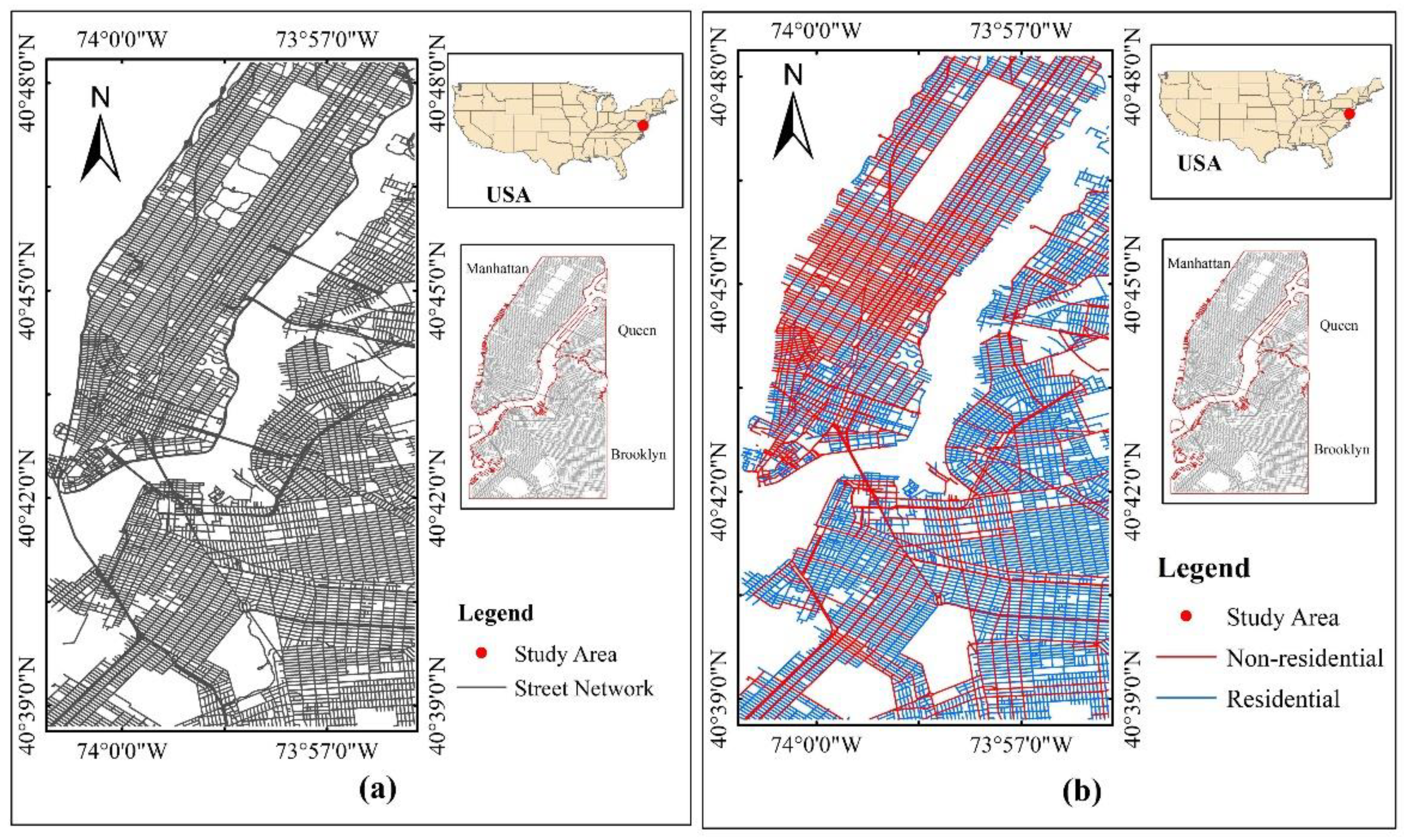
2.1. Study Area
2.2. Datasets
2.2.1. Remote Sensing Data
2.2.2. Social Sensing Data
- Trip ID: the unique ID of the trip
- Bike ID: the unique ID of the bike
- Departure Station ID: the unique ID of the station where people rent the bikes
- Departure Station Coordinate: the coordinates of the station where people rent the bikes
- Arrival Station ID: the unique ID of the station where people return the bikes
- Arrival Station Coordinate: the coordinates of the station where people return the bikes
- Departure Time: the time when a corresponding bike is rented by a person from a dock at the departure station
- Arrival Time: the time when a corresponding bike is returned by a person at a dock of the arrival station
- Trip ID: the unique ID of the trip
- Pick-Up Coordinate: the coordinates where the taxi picks up the passenger
- Drop-Off Coordinate: the coordinates where the taxi drops off the passenger
- Pick-Up Time: the time when a corresponding taxi picks up the passenger
- Drop-Off Time: the time when a corresponding taxi drops off the passenger
2.2.3. OSM Map
2.2.4. Class Definition
3. Method
3.1. Data Cleaning
3.2. Decision Tree
3.3. Random Forest
3.4. Training and Testing Sampling
3.5. Accuracy Assessment
4. Results and Discussion
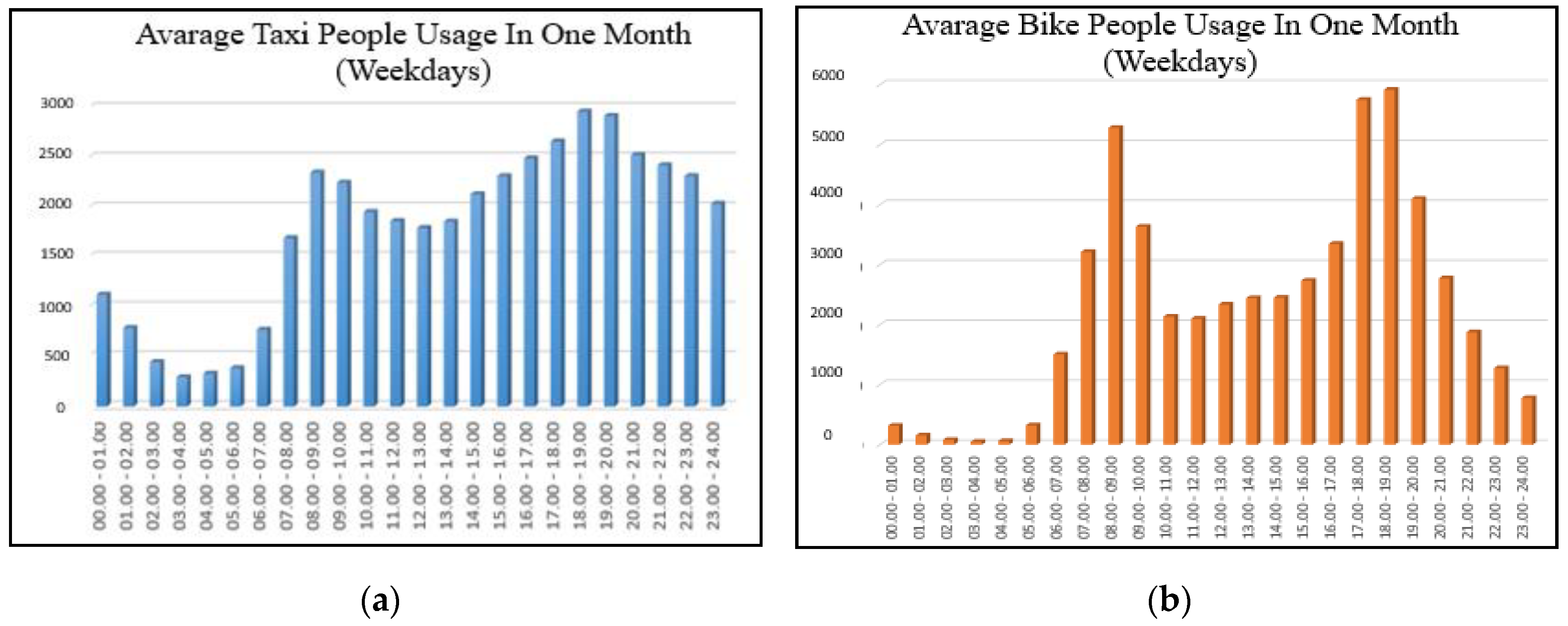
4.1. Temporal Analysis of Bike and Taxi Data
4.1.1. Weekday Time
4.1.2. Weekend Time
4.2. Spatial Analysis of Bike and Taxi Density Maps
4.2.1. Weekday Time
4.2.2. Weekend Time
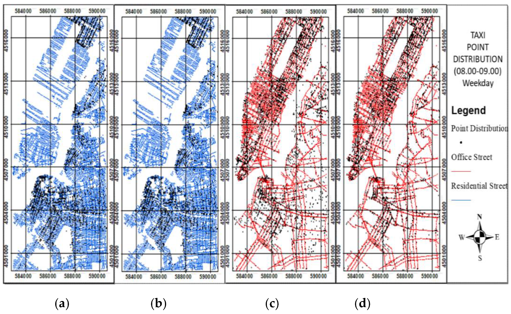
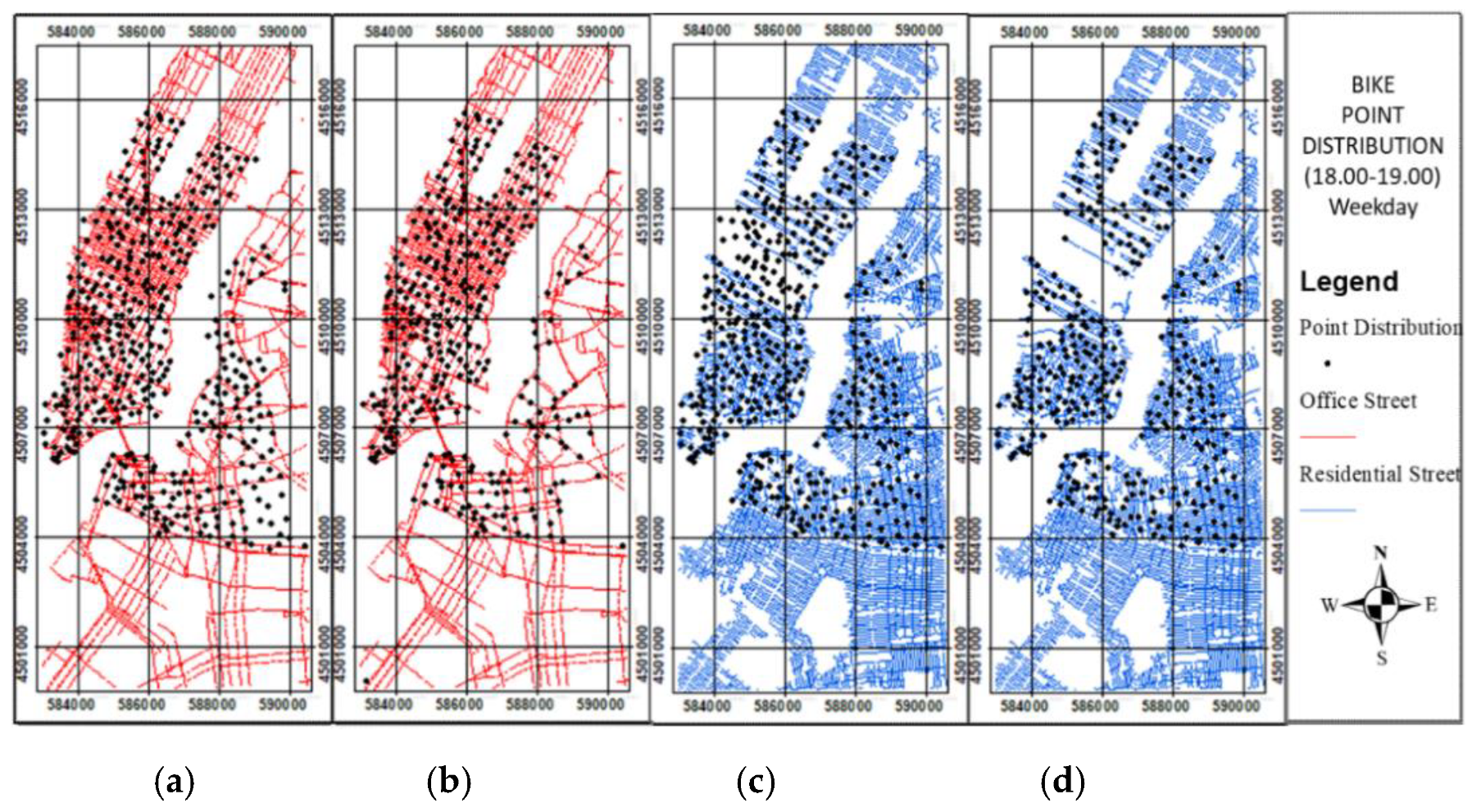
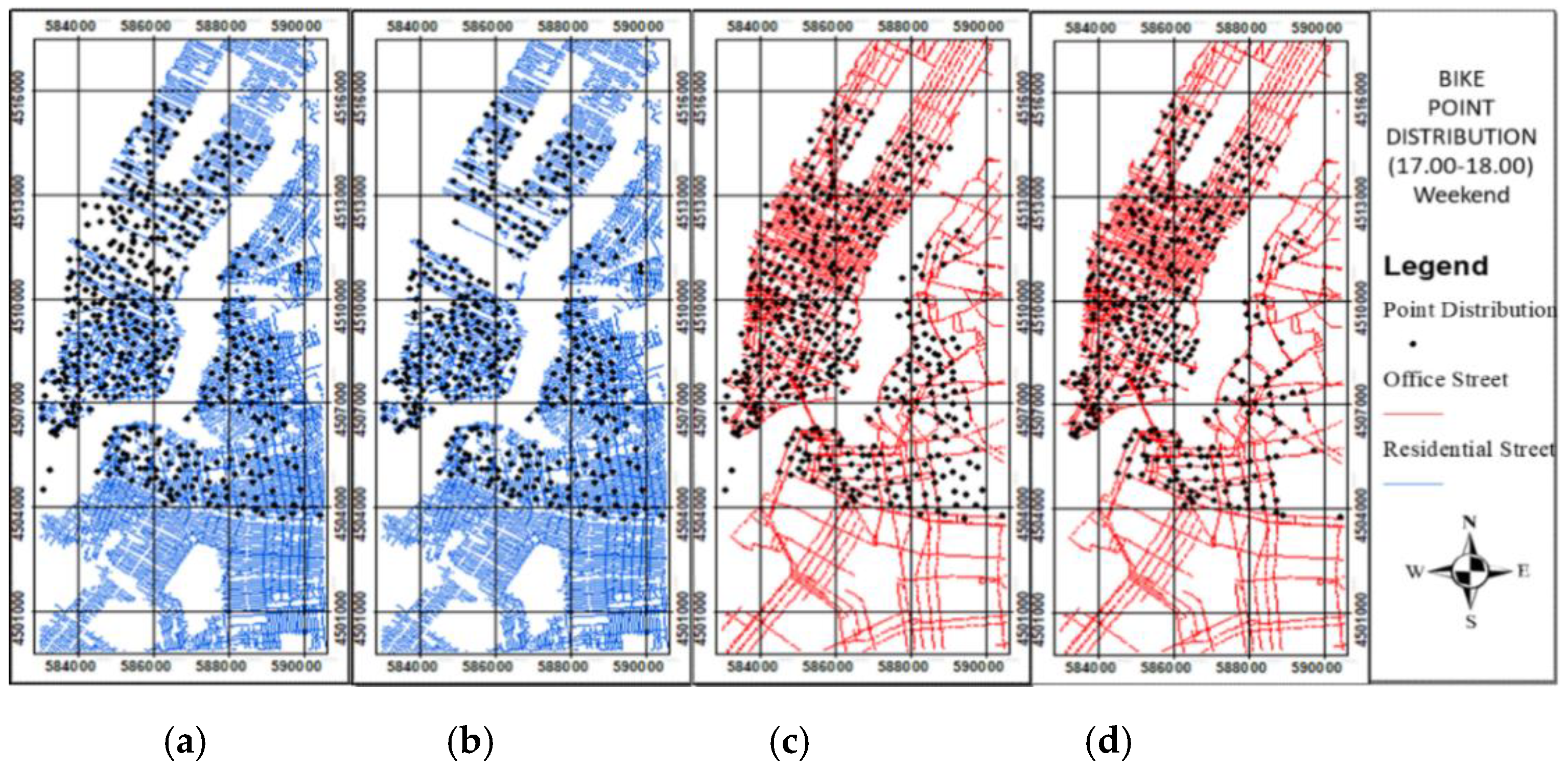
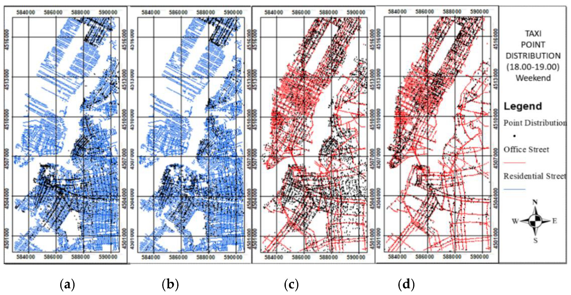
4.3. Effects of Data Cleaning on Point Distribution
4.3.1. Weekday Time
4.3.2. Weekend Time
4.4. Accuracy Assessment of Land Use Model
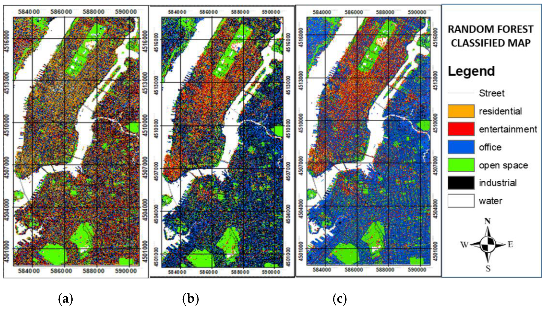
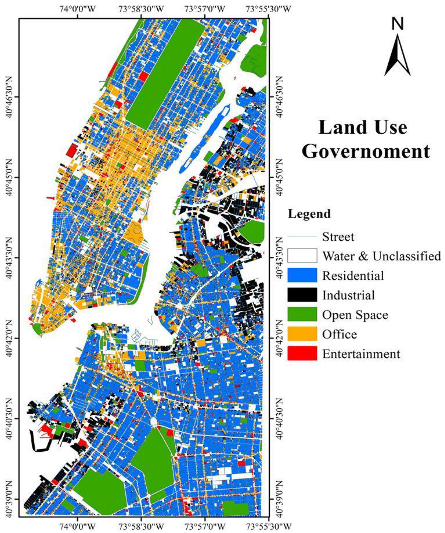
4.5. Urban Land Use Map
5. Conclusions
Author Contributions
Funding
Acknowledgments
Conflicts of Interest
Appendix A

| Actual Model | OpenSpace | Water | Industrial | Office | Entertainment | Residential | User’s Accuracy |
|---|---|---|---|---|---|---|---|
| OpenSpace | 44 | 3 | 3 | 0 | 0 | 4 | 81 |
| Water | 4 | 45 | 1 | 1 | 0 | 0 | 88 |
| Industrial | 0 | 0 | 34 | 0 | 7 | 8 | 69 |
| Office | 1 | 0 | 4 | 41 | 16 | 9 | 58 |
| Entertainment | 0 | 0 | 2 | 0 | 18 | 4 | 75 |
| Residential | 1 | 2 | 6 | 8 | 9 | 25 | 49 |
| Producer’s accuracy | 88 | 90 | 68 | 82 | 36 | 50 |
| Actual Model | OpenSpace | Water | Industrial | Office | Entertainment | Residential | User’s Accuracy |
|---|---|---|---|---|---|---|---|
| OpenSpace | 46 | 3 | 0 | 0 | 1 | 7 | 81 |
| Water | 4 | 45 | 0 | 1 | 0 | 0 | 90 |
| Industrial | 0 | 0 | 34 | 0 | 2 | 9 | 76 |
| Office | 0 | 0 | 4 | 40 | 6 | 2 | 77 |
| Entertainment | 0 | 0 | 5 | 4 | 36 | 0 | 80 |
| Residential | 0 | 2 | 7 | 5 | 5 | 32 | 63 |
| Producer’s accuracy | 92 | 90 | 68 | 80 | 72 | 64 |
| Actual Model | OpenSpace | Water | Industrial | Office | Entertainment | Residential | User’s Accuracy |
|---|---|---|---|---|---|---|---|
| OpenSpace | 46 | 5 | 0 | 0 | 0 | 0 | 90 |
| Water | 4 | 45 | 0 | 0 | 0 | 0 | 92 |
| Industrial | 0 | 0 | 39 | 1 | 2 | 1 | 91 |
| Office | 0 | 0 | 4 | 40 | 5 | 4 | 75 |
| Entertainment | 0 | 0 | 2 | 4 | 38 | 3 | 81 |
| Residential | 0 | 0 | 5 | 5 | 5 | 42 | 74 |
| Producer’s accuracy | 92 | 90 | 78 | 80 | 76 | 84 |
Appendix B
| Actual Model | OpenSpace | Water | Industrial | Office | Entertainment | Residential | User’s Accuracy |
|---|---|---|---|---|---|---|---|
| OpenSpace | 46 | 2 | 0 | 0 | 0 | 0 | 96 |
| Water | 4 | 45 | 0 | 1 | 0 | 0 | 90 |
| Industrial | 0 | 1 | 24 | 1 | 2 | 5 | 73 |
| Office | 0 | 2 | 12 | 40 | 32 | 12 | 41 |
| Entertainment | 0 | 0 | 7 | 8 | 14 | 14 | 33 |
| Residential | 0 | 0 | 7 | 0 | 2 | 19 | 68 |
| Producer’s accuracy | 92 | 90 | 48 | 80 | 28 | 38 |
| Actual Model | OpenSpace | Water | Industrial | Office | Entertainment | Residential | User’s Accuracy |
|---|---|---|---|---|---|---|---|
| OpenSpace | 46 | 2 | 0 | 0 | 0 | 0 | 96 |
| Water | 4 | 45 | 0 | 0 | 0 | 0 | 92 |
| Industrial | 0 | 2 | 36 | 4 | 2 | 8 | 69 |
| Office | 0 | 1 | 4 | 43 | 8 | 5 | 70 |
| Entertainment | 0 | 0 | 2 | 3 | 38 | 3 | 83 |
| Residential | 0 | 0 | 8 | 0 | 2 | 34 | 77 |
| Producer’s accuracy | 92 | 90 | 72 | 86 | 76 | 68 |
| Actual Model | OpenSpace | Water | Industrial | Office | Entertainment | Residential | User’s Accuracy |
|---|---|---|---|---|---|---|---|
| OpenSpace | 46 | 2 | 0 | 0 | 0 | 0 | 96 |
| Water | 4 | 45 | 0 | 0 | 0 | 0 | 92 |
| Industrial | 0 | 0 | 37 | 1 | 1 | 3 | 88 |
| Office | 0 | 0 | 6 | 43 | 6 | 1 | 77 |
| Entertainment | 0 | 0 | 2 | 4 | 41 | 1 | 85 |
| Residential | 0 | 3 | 5 | 2 | 2 | 45 | 79 |
| Producer’s accuracy | 92 | 90 | 74 | 86 | 82 | 90 |
References
- Jensen, J.R.; Cowen, D.C. Remote sensing of urban/suburban infrastructure and socio-economic attributes. In The Map Reader; John Willey & Sons, Ltd.: Hoboken, NJ, USA, 2011; pp. 153–163. [Google Scholar]
- Hu, S.; Wang, L. Automated urban land-use classification with remote sensing. Int. J. Remote Sens. 2012, 34, 790–803. [Google Scholar] [CrossRef]
- Herold, M.; Liu, X.; Clarke, K.C. Spatial Metrics and Image Texture for Mapping Urban Land Use. Photogramm. Eng. Remote Sens. 2003, 69, 991–1001. [Google Scholar] [CrossRef] [Green Version]
- Liu, Y.; Liu, X.; Gao, S.; Gong, L.; Kang, C.; Zhi, Y.; Chi, G.; Shi, L. Social Sensing: A New Approach to Understanding Our Socioeconomic Environments. Ann. Assoc. Am. Geogr. 2015, 105, 512–530. [Google Scholar] [CrossRef]
- D’Andrea, E.; Ducange, P.; Lazzerini, B.; Marcelloni, F. Real-Time Detection of Traffic From Twitter Stream Analysis. IEEE Trans. Intell. Transp. Syst. 2015, 16, 1–15. [Google Scholar] [CrossRef]
- Shin, D.; Aliaga, D.; Tuncer, B.; Arisona, S.M.; Kim, S.; Zünd, D.; Schmitt, G. Urban sensing: Using smartphones for transportation mode classification. Comput. Environ. Urban Syst. 2015, 53, 76–86. [Google Scholar] [CrossRef]
- Pan, G.; Qi, G.; Wu, Z.; Zhang, D.; Li, S. Land-Use Classification Using Taxi GPS Traces. IEEE Trans. Intell. Transp. Syst. 2013, 14, 113–123. [Google Scholar] [CrossRef]
- Jiang, S.; Alves, A.; Rodrigues, F.; Ferreira, J.; Pereira, F.C. Mining point-of-interest data from social networks for urban land use classification and disaggregation. Comput. Environ. Urban Syst. 2015, 53, 36–46. [Google Scholar] [CrossRef] [Green Version]
- Hu, T.; Yang, J.; Li, X.; Gong, P. Mapping Urban Land Use by Using Landsat Images and Open Social Data. Remote Sens. 2016, 8, 151. [Google Scholar] [CrossRef]
- Anugraha, A.S.; Chu, H.-J. Land Use Classification from Combined Use of Remote Sensing and Social Sensing Data. Int. Arch. Photogramm. Remote Sens. Spatial Inf. Sci. 2018, XLII-4, 33–39. [Google Scholar] [CrossRef]
- Haklay, M. How good is volunteered geographical information? A comparative study of OpenStreetMap and Ordnance Survey datasets. Environ. Plan. B Urban Anal. City Sci. 2010, 37, 682–703. [Google Scholar] [CrossRef] [Green Version]
- Schultz, M.; Voss, J.; Auer, M.; Carter, S.; Zipf, A. Open land cover from OpenStreetMap and remote sensing. Int. J. Appl. Earth Obs. Geoinf. 2017, 63, 206–213. [Google Scholar] [CrossRef]
- Jones, K. Importance of Land Cover and Biophysical Data in Landscape-Based Environmental Assessment; North America Land Cover Summit; Association of American Geographers: Washington, DC, USA, 2008; pp. 215–249. [Google Scholar]
- Thenkabail, P.S.; Schull, M.; Turral, H. Ganges and Indus river basin land use/land cover (LULC) and irrigated area mapping using continuous streams of MODIS data. Remote Sens. Environ. 2005, 95, 317–341. [Google Scholar] [CrossRef]
- Kasetkasem, T.; Arora, M.K.; Varshney, P.K. Super-resolution land cover mapping using a Markov random field based approach. Remote Sens. Environ. 2005, 96, 302–314. [Google Scholar] [CrossRef]
- Lambin, E.F.; Turner, B.L.; Geist, H.J.; Agbola, S.B.; Angelsen, A.; Bruce, J.W.; George, P. The causes of land-use and land-cover change: Moving beyond the myths. Glob. Environ. Chang. 2001, 11, 261–269. [Google Scholar] [CrossRef]
- Pal, M.; Mather, P. An assessment of the effectiveness of decision tree methods for land cover classification. Remote Sens. Environ. 2003, 86, 554–565. [Google Scholar] [CrossRef]
- Quinlan, J. Induction of Decision Trees. Mach. Learn. 1986, 1, 81–106. [Google Scholar] [CrossRef] [Green Version]
- Breiman, L.; Friedman, J.H.; Olshen, R.A.; Stone, C.J. Classification and Regression Trees; Wadsworth & Brooks/Cole Advanced Books & Software: Monterey, CA, USA, 1984. [Google Scholar]
- Mitchell, D.; Tom, M. Machine Learning; McGraw-Hill: New York, NY, USA, 1997. [Google Scholar]
- Liaw, A.; Wiener, M. Classification and regression by randomforest. R News 2002, 2, 18–22. [Google Scholar]
- Woznicki, S.A.; Baynes, J.; Panlasigui, S.; Mehaffey, M.; Neale, A. Development of a spatially complete floodplain map of the conterminous United States using random forest. Sci. Total Environ. 2019, 647, 942–953. [Google Scholar] [CrossRef] [PubMed]
- Zhang, M.; Chen, F.; Tian, B.; Liang, D. Multi-temporal SAR image classification of coastal plain wetlands using a new feature selection method and random forests. Remote Sens. Lett. 2018, 10, 312–321. [Google Scholar] [CrossRef]
- Chu, H.-J.; Wang, C.-K.; Kong, S.-J.; Chen, K.-C. Integration of full-waveform LiDAR and hyperspectral data to enhance tea and areca classification. GIScience Remote Sens. 2016, 53, 542–559. [Google Scholar] [CrossRef]
- Olofsson, P.; Foody, G.M.; Stehman, S.V.; Woodcock, C.E. Making better use of accuracy data in land change studies: Estimating accuracy and area and quantifying uncertainty using stratified estimation. Remote Sens. Environ. 2013, 129, 122–131. [Google Scholar] [CrossRef]
- Wang, Y.-D.; Wang, T.; Tsou, M.-H.; Li, H.; Jiang, W.; Guo, F. Mapping Dynamic Urban Land Use Patterns with Crowdsourced Geo-Tagged Social Media (Sina-Weibo) and Commercial Points of Interest Collections in Beijing, China. Sustainability 2016, 8, 1202. [Google Scholar] [CrossRef] [Green Version]
- Jiao, L. Urban land density function: A new method to characterize urban expansion. Landsc. Urban Plan. 2015, 139, 26–39. [Google Scholar] [CrossRef]


| Land Use Definition | Land Use Categories | Building Categories |
|---|---|---|
| Residential | One Family Dwelling | One Family Dwelling |
| Two Family Dwelling | Two Family Dwelling | |
| Walk Up Apartment | Walk Up Apartment | |
| Elevator Apartment | Elevator Apartment | |
| Condominium | ||
| Office | Office | Office |
| Entertainment | Commercial | Hotel |
| Theater | ||
| Store Building | ||
| Public Facilities | Churches | |
| Public Assembly and Cultural | ||
| Industrial | Industrial and Manufacturing | Warehouse |
| Factory and industrial building | ||
| Open space | Open space and Outdoor Recreation | Outdoor Recreation |
| Parks |
| Classification Method | Different Ways | Accuracy Assessment | |
|---|---|---|---|
| Overall Accuracy | Kappa Coefficient | ||
| Decision Tree | Use RS Only | 69% | 0.63 |
| Integration of RS and SS | 78% | 0.73 | |
| Without Data Cleaning | |||
| Integration of RS and SS | 83% | 0.80 | |
| With Data Cleaning | |||
| Random Forest | Use RS Only | 63% | 0.55 |
| Integration of RS and SS | 81% | 0.76 | |
| Without Data Cleaning | |||
| Integration of RS and SS | 86% | 0.82 | |
| With Data Cleaning | |||
© 2020 by the authors. Licensee MDPI, Basel, Switzerland. This article is an open access article distributed under the terms and conditions of the Creative Commons Attribution (CC BY) license (http://creativecommons.org/licenses/by/4.0/).
Share and Cite
Anugraha, A.S.; Chu, H.-J.; Ali, M.Z. Social Sensing for Urban Land Use Identification. ISPRS Int. J. Geo-Inf. 2020, 9, 550. https://doi.org/10.3390/ijgi9090550
Anugraha AS, Chu H-J, Ali MZ. Social Sensing for Urban Land Use Identification. ISPRS International Journal of Geo-Information. 2020; 9(9):550. https://doi.org/10.3390/ijgi9090550
Chicago/Turabian StyleAnugraha, Adindha Surya, Hone-Jay Chu, and Muhammad Zeeshan Ali. 2020. "Social Sensing for Urban Land Use Identification" ISPRS International Journal of Geo-Information 9, no. 9: 550. https://doi.org/10.3390/ijgi9090550
APA StyleAnugraha, A. S., Chu, H.-J., & Ali, M. Z. (2020). Social Sensing for Urban Land Use Identification. ISPRS International Journal of Geo-Information, 9(9), 550. https://doi.org/10.3390/ijgi9090550