Abstract
A slope unit is commonly used as calculation unit for regional landslide analysis. However, the capacity of the slope unit to reflect the geomorphological features of actual landslides still needs to be verified. This is because such accurate representation is critical to ensure the physical meaning of results from subsequent landslide stability analysis. This paper presents work conducted on landslides and slope extraction in two areas in China: The Jiangjia Gully area (Yunnan Province) and Fengjie County (Chongqing Municipality). Ground-based light detection and ranging (LiDAR) data are combined with field landslide terrace measurements to allow for the comparison of slope unit extraction methods (conventional vs. MIA-HSU) in terms of their ability to reflect the geomorphological features of shallow and deep-seated landslides. The results indicate that slope unit boundaries extracted by the conventional method do not match the geomorphological variations of actual landslides, and the method is therefore deficient in meaningfully extracting slope units for further landslide analysis. By contrast, slope units obtained using the MIA-HSU method accurately reflects the geomorphological features of both shallow and deep-seated landslides, and thus provides clearer geomorphological meaning and more reasonable calculation units for regional landslide assessment and prediction.
1. Introduction
A slope unit is commonly used as the calculation unit in regional landslide assessment and prediction [1,2,3,4,5]. Carrara (1988) first established the definition of a slope unit from the hydrological perspective [1]: a slope unit is a small hydrological region bounded by drainage and divide lines. A number of slope unit extraction methods have been proposed based on this definition, such as the r.slopeunits software [6,7], the curvature watershed method [8] and the texture watershed method [9]. Currently, the most widely used method includes the normal and inverse digital elevation model (DEM)-based hydrological process analysis (hereinafter referred to as the conventional method) [10,11,12,13,14,15,16]. However, all of these methods are based on surface hydrological process analysis, and slope units extracted by these methods cannot identify variations in slope gradient beyond the water flow direction. This results in the potential for abrupt changes in slope gradient to occur within a unit [5], and such abrupt changes mean that the slope unit may contain multiple inclined and flat regions. Thus, such extracted slope units cannot reflect the key geomorphological features and boundaries of actual landslides, such as the slope toe or the landslide terrace of a deep-seated landslide associated with distinct geomorphological variations [5,6,7,8].
Shallow and deep-seated landslides have different geomorphological features in nature. Shallow landslides occur at a smaller scale, with sliding masses <2–3 m thick [17,18,19,20,21,22,23]. In the field, multiple shallow landslides are often found at different locations on a slope with a homogenous gradient and aspect. Therefore, a shallow landslide can be approximated as having a homogenous slope gradient and aspect. To solve the defects in these methods above, Wang (2018) proposed a new slope unit extraction method MIA-HSU [5]. Slope units extracted by the MIA-HSU method have a homogenous slope gradient and aspect, satisfying the basic homogeneous assumption as required by landslide stability analysis. In the MIA-HSU method, such a slope with homogenous gradient and aspect is delineated into a slope unit, containing multiple shallow landslides that actually exist. In contrast, deep-seated landslides often occur at a large scale, with sliding masses up to tens of meters thick, and such a landslide may contain multiple landslide terraces and regions with distinct variations in slope gradient and aspect. Regions such as gently sloping terraces will become catchment areas during rainfall periods, affecting seepage patterns in the soil. Therefore, accurate slope extraction in these regions (including landslide terraces and distinct variations in geomorphology) allows for the effects of geomorphological variation to be accounted for in subsequent analysis of the infiltration process and ultimately on landslide stability.
In the present study, we investigated the capacity of slope units delineated by the conventional method and the MIA-HSU method to extract the geomorphological features of actual landslides, to provide calculation units that can truly reflect slope geomorphology for regional landslide prediction and assessment. To this end, an area prone to shallow landslides, known as the Jiangjia Gully area in Yunnan Province, China was selected, as well as an area prone to deep-seated landslides, in Fengjie County in the Three Gorges Reservoir area in Chongqing, China. The geomorphological information was acquired through LiDAR in combination with field measurements of actual landslide terraces. Slope units extracted by the conventional method and the MIA-HSU method are compared with the geomorphological features of actual landslides to validate the methodology.
2. Study Area
Shallow and deep-seated landslides are natural disasters that occur relatively frequently in the mountainous areas of southwestern China. Therefore, our two study areas were selected in terms of representing both shallow and deep-seated landslides in southwestern China. The Jiangjia Gully area in Yunnan Province, China, is prone to shallow landslides and debris flows. An observation and research station has been established by the Institute of Mountain Hazards and Environment, Chinese Academy of Sciences (Chengdu, Sichuan, China) in the Jiangjia Gully area, which provides a convenient survey environment for the shallow landslides in the area. Large-scale, deep-seated landslides in accumulated layers in the Three Gorges Reservoir area are of significant interest in landslide research, thus, we selected such a region in Fengjie County as area in which to study deep-seated landslides. These are mostly distributed on both sides of the Yangtze River and pose a threat to the lives of nearby residents and can seriously impact the shipping safety of the Yangtze River channel.
2.1. Shallow Landslides of the Jiangjia Gully Area
The Jiangjia Gully area is located in the northeastern part of Kunming, Yunnan, China (103°6′–103°13′ E and 26°13′–26°17′ N) (Figure 1a). This watershed is well-known as an area prone to shallow landslides and debris flows [5,23]. The region extends over an area of 47.1 km2 and is 12.1 km in length. The DEM with a cell size of 7 × 7 m that was generated from a 1:5000 topographic map [5] (Figure 1b). The climate is subtropical, with monsoons and a mean annual precipitation of 900 mm. Heavy rainfall occurs between May and October. The Jiangjia Gully area is located within a dry and hot valley area, with large terrain relief and elevations in the 1020–3250 m range above mean sea level. The bedrock mainly consists of gray slate, overlain by gravel soils.
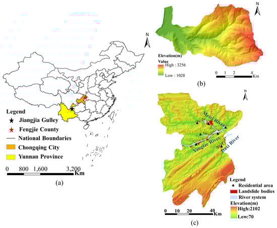
Figure 1.
Geographic location and DEM of the Jiangjia gulley area and Fengjie County, southwestern China. (a) the Geographic location of the Jiangjia gulley area and Fengjie County; (b) the DEM of the Jiangjia gulley area; and (c) the DEM of the Fengjie county.
2.2. Deep-seated Landslides of Fengjie County
The county of Fengjie is located in the northeastern part of Chongqing (109°1′17″–109°45′5″ E, 30°29′19″–31°22′23″ N; Figure 1a). The total land area is 4080 km2, extending 70 km in an east–west direction and 95 km in a north–south direction (Figure 1c). The DEM of Fengjie county with 20 m resolution is shown in Figure 1b. This area experiences a subtropical and humid monsoon climate, with a mean annual precipitation of 1145 mm [24,25]. Precipitation is mostly concentrated between July and September, accounting for 42% of the total annual precipitation. The terrain has a large elevation range, from 70 to 2100 m above mean sea level [25]. The geology consists mainly of limestone and sandstone and outcrops consist of mid-Triassic Badong Formation strata, with a broken and loose structure [25]. Rivers in the area drain into the Yangtze River system. The Yangtze River extends for 45 km through this area, of which the main tributaries are the Meixi and Daxi Rivers. This area is prone to geological disasters, with many large-scale, deep-seated and loose accumulated layer landslides distributed along the Yangtze River system. Landslides in the area not only affect the safety of nearby residents, but may also obstruct shipping channels in the river. The comparison of the Jiangjia gulley area and Fengjie county is shown in Table 1.

Table 1.
The comparison of the Jiangjia Gulley area and the Fengjie county ([5,23,25]).
3. Methodology
3.1. The Slope Unit Extraction Method MIA-HSU
The MIA-HSU method proposes a new definition of the slope unit: a continuous, homogeneous and closed small region in three-dimensional (3D) space, the slope gradient and aspect of which is homogeneous and contains no abrupt change in slope gradient within it [5]. Such a definition meets the basic requirements of slope unit homogeneity needed for landslide stability analysis [26,27,28,29]. This definition not only satisfies the homogeneity requirement of the physical landslide model, but also matches the terrain relief features. Based on this definition, the MIA method uses logical algorithms, such as expansion and erosion, to extract slope units. Slope units extracted by this method presents a more uniform slope and is able to identify geographic features that are meaningful for further landslide analysis [5].
The MIA-HSU method adopts morphological image analysis to extract the morphological skeletons of ridges and valleys that reflect slight terrain relief characteristics. A morphological skeleton describes how a certain imaged region is refined into a central skeleton to eliminate most of the redundant information, without changing image connectivity or topological structure. A morphological skeleton accurately describes the geometric features of the original image and it can be widely applied in object identification and geometric morphological analysis. The maximum disc method was adopted in this present study to extract the morphological skeleton. The principle of this method is as follows: a series of discs with variable diameter are set at tangents to the image contours and, if no larger circles within the image can be found to completely include these discs, the centers of these discs are connected to form the skeleton (Figure 2a,b). Combined with the image processing toolbox in Matlab, morphological skeletons are extracted from the binary images of valleys (Figure 3a,b) to reflect geometric features of ridges and valleys. The extracted morphological skeletons of ridges and valleys accurately match slight variations in the geomorphological features (Figure 3c,d).
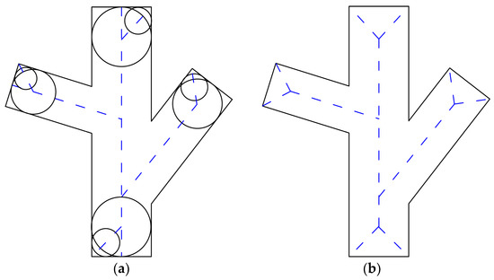
Figure 2.
Schematic diagrams of the morphological skeleton algorithm showing (a) different positions of maximum disk sizes and (b) the whole skeleton, indicated with dashed lines.
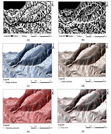
Figure 3.
Morphological ridge and valley skeletons showing (a) binary image with valleys shown in white, (b) binary image with ridges shown in white, (c) morphological skeleton of valleys over shaded relief, (d) morphological skeleton of ridges over shaded relief, (e) closed morphological skeleton network in which each small region contains homogenous geomorphological features and (f) slope unit extracted by MIA-HSU method.
3.2. The Conventional Slope Unit Extraction Method
The conventional method defines the slope units as the left and right banks of each sub-watershed within a watershed [2,30]. Based on this definition, slope units are extracted from a digital elevation model (DEM) using a GIS-based method of hydrological process analysis [11]. The key process for slope unit extraction lies in the identification of the ridge line and divide lines of a watershed. This conventional method uses the normal DEM to calculate the low direction and flow accumulation, then generate the ridge lines. Because there is no way to generate all parts of drainage lines through normal DEM, the reverse DEM is used to obtain the drainage lines of the actual terrain. The actual terrain is then divided into a series of sub-watersheds along drainage lines and mountain ridge lines, and the slope is extracted from the left and right banks of each sub-watershed to obtain two slope units (Figure 4).
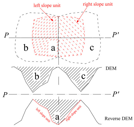
Figure 4.
Schematic diagram of slope unit definition from the conventional method (reverse DEM = DEM rotated by 180° along the horizontal plane A-A′). Thus, high DEM values are turned into low values, and low DEM values are turned into high values, and the original drainage line is turned into a ridge line. “a” represents a sub-watershed obtained from the DEM data, and “b” and “c” are the watersheds obtained by the reverse DEM.
3.3. The Extraction of Geomorphological Features of Landslides Using Slope Units
3.3.1. The Ability of Slope Unit to Reflect the Terrain Features of Shallow Landslide
In a field environment, a shallow landslide has uniform slope and small scale, and it is often found that several shallow landslides occurred on a slope with homogenous gradient and aspect. Therefore, this paper verifies the capacity of slope units to shallow landslides:
- the slope unit should contain several actual shallow landslides;
- the slope unit should have homogeneity slope gradient.
3.3.2. The Ability of Slope Unit to Extract the Terrain Regions of Deep-Seated Landslide
According to the variation of terrain, the deep-seated landslide can be divided into many terrain regions with different slope gradient and aspect. If the slope unit and terrain region can overlap completely, it means the slope unit can accurately extract the terrain features of deep-seated landslide. Therefore, this paper uses the area overlap degree i to verify the ability of slope unit to extract the terrain regions. The area overlap degree i is calculated as follows:
where i is the area overlap degree of the slope unit and Terrain region; As is the area of slope unit; AT is the area of terrain region; As ∩ AT Means the overlap area of slope unit and Terrain region, which can be calculated by ArcGIS.
4. Geomorphology of Shallow Landslides Extracted from Slope Units
4.1. Boundary Identification
The shallow landslide boundary identification was conducted using a field-based LiDAR survey in the Jiangjia Gully area. The LiDAR technique is characterized by high spatial resolution, high anti-interference capabilities and is largely automated. It can rapidly acquire high-precision terrestrial 3D models and can be applied to landslide identification, dynamic landslide deformation monitoring and acquisition of geomorphological features [31,32]. The LiDAR system is composed of a 3D laser scanning system, a control system and a power supply system [33,34,35,36]. The complete 3D laser scanning system includes a laser ranging and angle measuring system, a laser scanning system, an integrated charge-coupled device camera, and an internal control and correction system. The control system mainly consists of a personal computer and built-in data processing software for recording and processing point cloud data during the scanning process.
Deposits in the middle and lower reaches of the Jiangjia Gully area are relatively thick and slopes have gradients of 30° to 40°. Sliding in this region is induced by rainfall, resulting in typically shallow landslides [5]. Therefore, identification of the landslide-prone areas was carried out in the middle and lower reaches of the Jiangjia Gully area. Differential Global Positioning System (DGPS) base stations were deployed in the field to improve the positioning accuracy of the observation points (Figure 5a). Observation points were measured using LiDAR scanners (Figure 5b) which were distributed in the field as shown in Figure 6a. Note that the different shadings indicate the maximum vertical error within the range of scanning. The maximum vertical error within the range of scanning was <400 mm (Figure 6b), indicating an acceptable density of observation points. The point cloud data obtained by 3D scanning contains information such as 3D coordinates, reflection intensity, and color (Figure 6b). As such, different objects are distinguished based on color and intensity. A high-resolution DEM is obtained from the point cloud data and is then used for qualitative and quantitative landslide boundary delineation.
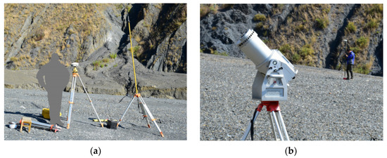
Figure 5.
Ground LiDAR survey in the Jiangjia Gully area showing (a) DGPS base station (b) RIEGL Z-6200 laser scanner.
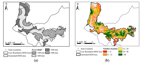
Figure 6.
Point cloud data collection and processing in Jiangjia Gully area showing (a) data acquisition points with error fields and (b) point cloud data obtained from scanning, with density of points shown.
4.2. Comparison of Extraction Results
A total of 19 shallow landslide regions were extracted and identified in the middle and lower reaches of the Jiangjia Gully area using ground-based LiDAR (Figure 7). The active shallow landslide regions are indicated with crosshatching. Then, slope unit boundaries extracted using both the MIA-HSU and conventional methods (Figure 7a,b) were compared with the actual shallow landslide boundaries identified by LiDAR. As shown in Figure 7a,b, Slope units extracted by the MIA-HSU and conventional method both contains multiple shallow landslides, the shallow landslide number contained in each slope unit is shown in Table 2.
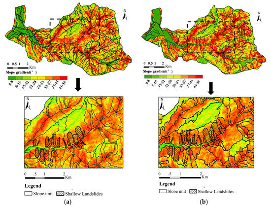
Figure 7.
Topographic feature extraction for shallow landslides in Jiangjia Gully area showing results from (a) The MIA-HSU method and (b) The conventional method.
Table 2.
The shallow landslide contained in slope units.
Slope units extracted by the MIA-HSU method show relatively homogenous slope gradients, and each contains multiple shallow landslides (Figure 7a). Although the slope units extracted by the conventional method also contained several shallow landslides, very abrupt changes in slope gradient were present within units (Figure 7b), indicating distinct geomorphological variations within the slope units. This phenomenon was particularly evident in the middle and lower parts of the DEM. The smaller standard deviation of slope gradient in a slope unit indicates lower amplitude of variation of slope gradient. A comparison of slope standard deviation results is shown in Figure 8. For slope units extracted by the conventional method, the standard deviation of the slope is in the 3.5°–14.5° range. However, for MIA-HSU the standard deviation of the slope is in the 4.5°–8.5° range. These results indicate that the conventional method is associated with a larger fluctuation in slope gradient.
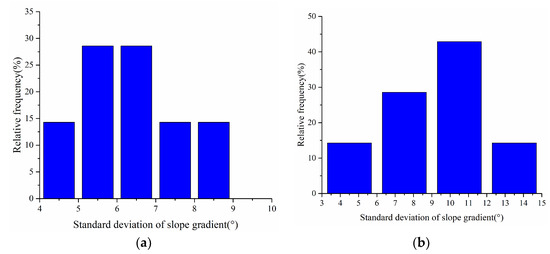
Figure 8.
Standard deviation of slope gradient of slope unit; (a) the MIA-HSU method and (b) the conventional method.
The comparison indicates that there is distinct terrain relief within slope units extracted by the conventional method, which therefore does not meet the requirement for slope gradient homogeneity. However, slope units extracted using MIA-HSU accurately reflect the geomorphological features of shallow landslides while satisfying the requirement for slope gradient homogeneity.
5. Geomorphology of Deep-seated Landslides Extracted from Slope Units
5.1. Measurement of Landslide Geomorphology
In September 2017, a field survey was carried out at the Xinpu landslide which threatened the safety of the Yangtze River channel, and the Jijing landslide which threatened the Meixi River channel. A hand-held GPS and a tacheometer were used to measure the latitude, longitude, and geometry of landslide terraces and places showing abrupt changes in slope gradient. Particular measurement points were then marked on Google Earth and landslide terraces and regions showing homogenous slope gradients and aspects of the landslide were extracted.
5.1.1. Geomorphological Results from the Xinpu Landslide
The Xinpu landslide is located on the right bank of the Yangtze River (109°21′09′’–109°21′50′’ E and 30°57′23′’–30°58′24′’ N) and covers a total area of 2.45 km2 with a volume of 4.0 × 10⁷ m3. The landslide has a narrow apex and broad base, with an elevation of 81–85 m above mean sea level at the front edge and 810–830 m at the rear edge. The Xinpu landslide is a large-scale, deep-seated landslide, consisting of three landslide terraces from top to bottom: Daping landslide terrace, Shangertai landslide terrace and Xiaertai landslide terrace (T1, T2, and T3 in Figure 9a, respectively).The measurement points were marked on Google Earth to obtain the geomorphological features of the Xinpu landslide (Figure 10). The centroid point and area of landslide terrace 1–3 is shown in Table 3.
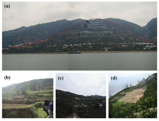
Figure 9.
Photographs of the Xinpu landslide showing (a) front view, (b) Daping landslide terrace (T1), (c) Shangertai landslide terrace (T2) and (d) Xiaertai landslide terrace (T3).
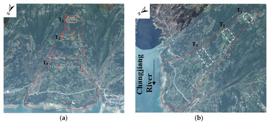
Figure 10.
Geomorphological features of the Xinpu landslide showing (a) front view and (b) lateral view (the measuring points are marked with red stars).
Table 3.
The measurement result of landslide terrace 1–3 in the Xinpu landslide.
5.1.2. Geomorphological Results from the Jijing Landslide
The Jijing landslide is located on the left bank of the Meixi River (109°28′25.67′’–109°29′55.27′’ E and 31°06′22.49′’–31°07′33.58′’ N). The total area of the landslide is 5.08 km2 and the volume is 1.25 × 10⁸ m3. The elevation of the landslide is 171–183 m above mean sea level at the front edge and 570–610 m at the rear edge. It is a large, deep-seated landslide with multiple landslide terraces and areas with distinct variation in slope gradient. The measurement points were marked on Google Earth to obtain geomorphological features (Figure 11). Seven terrain regions were extracted from this landslide (Figure 11). Those numbered one to six indicate regions with relatively homogenous slope gradient and aspect; the number seven indicates a landslide terrace named Ma’anqiao, and distinct slope gradient changes exist between adjacent regions. The coordinate of centroid point(x, y) and area of each terrain region is shown in Table 4.
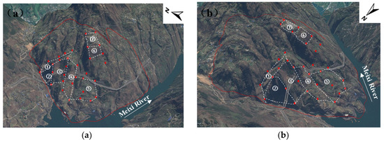
Figure 11.
Geomorphological features of the Jijing landslide showing (a) front view and (b) lateral view (the measuring points are marked with red stars).
Table 4.
Jijing landslide measurement result.
5.2. Comparison of the Extraction Results
5.2.1. Geomorphology of the Xinpu Landslide Extracted from Slope Units
Slope units of the Xinpu landslide were extracted using both the conventional and MIA-HSU methods (Figure 12). To ensure rational comparison of results, a similar number of slope units were extracted using each method. The slope units extracted using MIA-HSU clearly identified the three landslide terraces of the Xinpu landslide (Figure 12a,b), and the extraction results were available for subsequent landslide analysis with no need for manual correction. The overlap degree of area of slope unit and landslide terraces 1–3 is shown in Table 5. As shown in Table 5, the range of overlap degree i is 63.15%–86.67%. However, the slope units extracted by the conventional method failed to show the landslide terraces or other regions with abrupt changes in slope gradient (Figure 12c,d). These extraction results were disordered, with many small, disconnected units and unreasonably long strip-like units emerging, which required extensive manual correction.
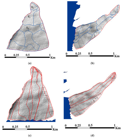
Figure 12.
Geomorphological features of the Xinpu landslide based on slope unit extraction: (a) front view and (b) lateral view of slope units from the MIA-HSU method; (c) front view and (d) lateral view of slope units from the conventional method. Note that the three landslide terraces shown in Figure 6 (T1, T2, and T3) were extracted using the MIA-HSU method, which is not the case for the conventional method.
Table 5.
Area overlap degree of area of slope unit and landslide terraces 1–3 of the Xinpu landslide.
5.2.2. Geomorphology of the Jijing Landslide Extracted from Slope Units
Figure 13 shows the results of slope unit extraction on the Jijing landslide by both the conventional and MIA-HSU methods. A total of 29 slope units were extracted using the MIA-HSU method, while 34 units were extracted using the conventional method. Numbers one to seven in the slope units from MIA-HSU extraction (Figure 13a,c) correspond to numbers one to seven extracted from field measurement (Figure 7). The overlap degree of area of slope unit and terrain region is shown in Table 6. As shown in Table 6, the range of overlap degree i is 61.11%–93.75%. This indicates that the slope units ably reveal landslide terraces and regions with abrupt changes in slope gradient within the landslide and, thus, demonstrate clear geomorphological meaning.
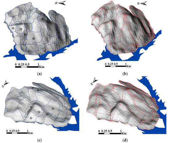
Figure 13.
Results of terrain characteristic extraction from the Jijing landslide: (a) front view and (b) lateral view of slope units from the MIA-HSU method; (c) front view and (d) lateral view of slope units from the conventional method (Numbers one to seven in the slope units from MIA-HSU extraction correspond to numbers one to seven extracted from field measurement in Figure 10).
Table 6.
The overlap degree of area of slope unit and terrain regions in Jijing landslide.
In contrast, the conventional method, which is based on surface hydrological process analysis, was not able to identify variations in slope gradient outside of the water flow direction. As a result, the conventional extraction method produced results containing a series of long, narrow polygons (Figure 13b,d). Therefore, such slope units do not provide evidence of landslide terraces or other regions containing abrupt changes in slope gradient, thereby failing to extract the precise geomorphological features of the slope.
6. Discussion
6.1. Geomorphological Meaning of Slope Units Extracted by MIA-HSU
The MIA-HSU method defines slope units from the perspective of terrain homogeneity, and thus defines regions with homogeneous slope gradient and aspect. The different definitions of slope units therefore result in the two methods using different techniques to extract geomorphological features of a slope. The conventional method defines slope units based on hydrology, a terrain region bounded by drainage and divide lines. Therefore, the normal and reversed DEM are used to extract the drainage and divide lines, respectively. The drainage and divide lines of Jijing landslide is shown in Figure 14a,b. The drainage and divide lines only takes into account the effects of hydrological conditions on landslide formation and overlooks the terrain relief features within the slope. The region bounded by drainage and divide lines can be a single slope or multiple slopes.
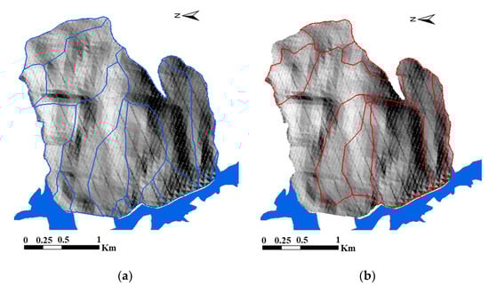
Figure 14.
The slope unit extraction process of conventional method of Jijing landslide: (a) the divide lines extracted from normal DEM and (b) the drainage lines extracted from reverse DEM.
The MIA-HSU method uses Morphological technology to extract the Morphological skeleton of valleys and ridges, as shown in Figure 15a, and the Morphological skeleton can accurately reflect the terrain relief in the Jijing landslide. As shown in Figure 15b, the closed morphological skeleton network in which each small region contains homogenous terrain characteristics. Therefore, the slope units extracted using the MIA-HSU method have clearer geomorphological meaning compared with those extracted by the conventional method. Fundamentally, this discrepancy is related to the different definitions of slope units between these two methods.
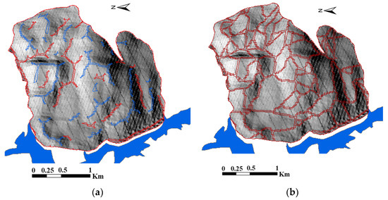
Figure 15.
The slope unit extraction process of MIA-HSU method of Jijing landslide: (a) morphological skeleton of valleys and ridges over shaded relief and (b) closed morphological skeleton network in which each small region contains homogenous geomorphological features.
6.2. Potential and Limitations for Regional-scale Application of MIA-HSU
In the MIA-HSU method, the field survey and measurement of actual landslides are used to calibrate the slope unit result. The slope unit delineation results were repeatedly compared with actual geomorphological features to evaluate whether slope unit can accurately reflect the geomorphological features of actual landslides. After multiple comparisons, the extracted slope unit result accurately reflects the actual geomorphological features while satisfying the requirement for slope gradient homogeneity. For the purpose of landslide risk assessment and prediction using slope unit, detailed geological survey is also necessary to achieve the stratum and lithology information within the slope unit, in order to generate the geological model and calculation profile of each slope unit [10,13,37]. Then, appropriate analysis method (statistics or physical-based method) can be used to analysis the stability of each slope unit; by this way, the slope unit can be applied to the risk assessment and prediction of regional landslides.
However, the MIA-HSU method may still be subject to some limitations in regional-scale applications:
- 1.
- The results of slope unit extraction are affected by the DEM resolution
All existing slope unit extraction methods use DEM as input data, the resolution of which affects the extraction results. If all other input parameters are fixed in the MIA-HSU method, the higher the DEM resolution, the larger the number of slope units extracted, and the better the slope unit boundary can match the terrain characteristics of actual landslides. By contrast, the lower the DEM resolution, the smaller the number of slope units extracted, and the rougher the extraction results obtained. Therefore, application of this method is not ideal in those areas for which high-resolution DEM data are not available.
- 2.
- The results of slope unit extraction are affected by artificially set thresholds
In the MIA-HSU method, some thresholds are set by the user based on experience (e.g., maximum and minimum area thresholds of the slope unit) as control conditions for the extraction results. The smaller the maximum area threshold set by the user, the larger the number of slope units obtained. These user-defined threshold settings are subjective to a certain degree, which can negatively affect the reproducibility of the extracted results.
- 3.
- A simple and easy method is lacking for optimization of extraction results
The MIA-HSU method depends on field surveys of geomorphological features of landslides for optimization of the extraction results. In other words, the geomorphological features of actual landslides are measured in the field, then user-defined thresholds (e.g., the maximum and minimum area threshold) are continually adjusted to obtain different slope unit delineation results. These results are repeatedly compared with actual terrain characteristics to ensure the slope units accurately reflect the geomorphological features. This evidently requires fieldwork and repeated laboratory calculations, with associated investments of time and effort. Further studies are needed to identify a more efficient means of optimizing slope unit extraction.
7. Conclusions
The physical characteristics of a slope unit must accurately reflect the geomorphological features of actual landslides. This is critical to ensure that the results of subsequent landslide stability analysis have practical physical meaning, and that the location of impending landslides can be identified accurately based on predictions from slope units. However, due to the different definitions of the slope unit, the extraction method is various. The ability of slope units to reflect geomorphological features of landslides when they are extracted by different methods remains unclear. In the present study, comparisons have been made between slope units extracted by the conventional method and those extracted by the MIA-HSU method, with the aim of evaluating whether they accurately reflect geomorphological features of both shallow and deep-seated landslides. The data were collected using ground-based LiDAR and field measurements of landslide terraces. From the data and the comparisons, the following conclusions can be drawn:
- Extraction results from the shallow landslide area show that multiple small-scale shallow landslides were enclosed within slope units extracted by both the conventional and MIA-HSU methods. The standard deviation of the slope is in the 3.5°–14.5° range using conventional method, while the standard deviation of the slope is in the 4.5°–8.5° range using MIA-HSU. These results indicate that distinct variations in slope gradient within the slope units were noted when extracted using the conventional method. This conventional method failed to meet the basic assumption of homogeneity as a premise for the physical model. By contrast, slope units extracted by the MIA-HSU method not only reflected the geomorphological features of shallow landslides, but also showed relatively homogenous slope gradients within each unit, which has improved application in landslide analysis models.
- Extraction results from the deep-seated landslide area show that slope units extracted by the conventional method cannot extract and identify the landslide terrace and terrain regions, while the slope unit boundaries failed to match the geomorphological variations of the landslides. By contrast, the slope units extracted using MIA-HSU can extract the landslide terrace and terrain regions more accurately. The range of overlap degree between slope unit and landslide terrace is 63.15%–86.67%, while the range of overlap degree of slope unit and terrain region is 61.11%–93.75%. Therefore, slope units extracted using MIA-HSU have a clearer geomorphological meaning.
Overall, it has been shown that slope units extracted by the MIA-HSU method not only meet the basic requirement of the physical model for homogeneity within prediction units, but also accurately reflect the geomorphological features of both shallow and deep-seated landslides. Additionally, the automatic extraction procedure of the MIA-HSU method is more convenient than the conventional method and automated output of raster data of the slope units is possible once the DEM raster data have been analyzed. Thus, the MIA-HSU method is a promising tool for slope unit extraction at a regional scale in landslide assessment and prediction.
Author Contributions
Kai Wang and Shaojie Zhang extract the slope unit and made the field investigation; Hui Xu and Fangqiang Wei proposed the methodology; Hui Xu and Wanli Xie analyzed the data; Kai Wang organized and wrote this paper. All authors have read and agreed to the published version of the manuscript.
Funding
This research was funded by the Strategic Priority Research Program of the Chinese Academy of Sciences (XDA23090202), the Key Scientific Research project of Higher Education Institutions, Henan Province, China (20A560024), the Chongqing Municipal Bureau of Land, Resources and Housing Administration (KJ-2019054) and Key technologies for monitoring and early warning of intelligent meteorological and geological disasters in the Three Gorges reservoir area (cstc2018jscx-mszdX0074).
Conflicts of Interest
The authors declare no conflict of interest.
References
- Carrara, A. Drainage and divide networks derived from high-fidelity digital terrain models. In Quantitative Analysis of Mineral and Energy Resources; Springer: Dordrecht, The Netherlands, 1988; pp. 581–597. [Google Scholar]
- Carrara, A.; Guzzetti, F. Geographical information systems in assessing natural hazards. Adv. Nat. Technol. Hazards 1995, 4, 45–59. [Google Scholar] [CrossRef]
- Giles, P.T.; Franklin, S.E. An automated approach to the classification of the slope units using digital data. Geomorphology 1998, 21, 251–264. [Google Scholar] [CrossRef]
- Akagunduz, E.; Erener, A.; Ulusoy, I.; Duzgun, H.S.B. Deliniation of Slope Units based on Scale and Resolution Invariant 3D Curvature Extraction. In Proceedings of the Geoscience and Remote Sensing Symposium, 2008, IGARSS 2008, IEEE International 2008, Boston, MA, USA, 7–11 July 2008; Volume 3, pp. III-581–III-584. [Google Scholar]
- Wang, K.; Zhang, S.; DelgadoTéllez, R.; Wei, F. A new slope unit extraction method for regional landslide analysis based on morphological image analysis. Bull. Eng. Geol. Environ. 2019, 78, 4139–4151. [Google Scholar] [CrossRef]
- Alvioli, M.; Marchesini, I.; Fiorucci, F.; Ardizzone, F.; Rossi, M.; Reichenbach, P.; Guzzetti, F. Automatic delineation of geomorphological slope units. In Proceedings of the EGU General Assembly Conference Abstracts, Vienna, Austria, 27 April–2 May 2014; Volume 16. [Google Scholar]
- Alvioli, M.; Marchesini, I.; Reichenbach, P.; Rossi, M.; Ardizzone, F.; Fiorucci, F.; Guzzetti, F. Automatic delineation of geomorphological slope units with r. slopeunits v1. 0 and their optimization for landslide susceptibility modeling. Geosci. Model Dev. 2016, 9, 3975. [Google Scholar] [CrossRef]
- Yan, G.; Liang, S.; Zhao, H. An Approach to Improving Slope Unit Division Using GIS Technique. Sci. Geogr. Sin. 2017, 37, 1764–1770. (In Chinese) [Google Scholar]
- Cheng, L.; Zhou, B. Slope unit extraction algorithm based on texture watershed. J. Comput. Appl. 2019, 6, 1810–1815. (In Chinese) [Google Scholar] [CrossRef]
- Xie, M.W.; Zhou, G.Y.; Esaki, T. GIS component based 3D landslide hazard assessment system: 3DSlopeGIS. Chin. Geogr. Sci. 2003, 13, 66. [Google Scholar] [CrossRef]
- Turel, M.; Frost, J.D. Delineation of slope profiles from digital elevation models for landslide hazard analysis. Am. Soc. Civil. Eng. 2011, 829–836. [Google Scholar] [CrossRef]
- Jia, N.; Mitani, Y.; Xie, M.; Djamaluddin, I. Shallow landslide hazard assessment using a three-dimensional deterministic model in a mountainous area. Comput. Geotech. 2012, 45, 1–10. [Google Scholar] [CrossRef]
- Jia, N.; Mitani, Y.; Xie, M.; Tong, J.; Yang, Z. GIS deterministic model-based 3D large-scale artificial slope stability analysis along a highway using a new slope unit division method. Nat. Hazards 2015, 76, 873–890. [Google Scholar] [CrossRef]
- Zhou, S.; Fang, L.; Liu, B. Slope unit-based distribution analysis of landslides triggered by the April 20, 2013, Ms 7.0 Lushan earthquake. Arab. J. Geosci. 2015, 8, 7855–7868. [Google Scholar] [CrossRef]
- Zhuang, J.; Peng, J.; Xu, Y.; Xu, Q.; Zhu, X.; Li, W. Assessment and mapping of slope stability based on slope units: A case study in Yan’an, China. J. Earth Syst. Sci. 2016, 125, 1439–1450. [Google Scholar] [CrossRef]
- Schlögel, R.; Marchesini, I.; Alvioli, M.; Reichenbach, P.; Rossi, M.; Malet, J.P. Optimizing landslide susceptibility zonation: Effects of DEM spatial resolution and slope unit delineation on logistic regression models. Geomorphology 2018, 301, 10–20. [Google Scholar] [CrossRef]
- Terlien, M.T. The determination of statistical and deterministic hydrological landslide-triggering thresholds. Environ. Geol. 1998, 35, 124–130. [Google Scholar] [CrossRef]
- Van Asch, T.W.; Buma, J.; Van Beek, L.P.H. A view on some hydrological triggering systems in landslides. Geomorphology 1999, 30, 25–32. [Google Scholar] [CrossRef]
- Delmonaco, G.; Margottini, C.; Martini, G.; Paolini, S.; Spizzichino, D. Large scale shallow landslides hazard assessment of the Inca Historical Sanctuary area (Peru). In Proceedings of the EGU General Assembly Conference Abstracts, Vienna, Austria, 19-24 April 2009; Volume 11, p. 8076. [Google Scholar]
- Giannecchini, R. Relationship between rainfall and shallow landslides in the southern Apuan Alps (Italy). Nat. Hazards Earth Syst. Sci. 2006, 6, 357–364. [Google Scholar] [CrossRef]
- Meisina, C.; Scarabelli, S. A comparative analysis of terrain stability models for predicting shallow landslides in colluvial soils. Geomorphology 2007, 87, 207–223. [Google Scholar] [CrossRef]
- Cohen, D.; Lehmann, P.; Or, D. Fiber bundle model for multiscale modeling of hydromechanical triggering of shallow landslides. Water Resour. Res. 2009, 45. [Google Scholar] [CrossRef]
- Zhang, S.J.; Xu, C.X.; Wei, F.Q.; Hu, K.H.; Xu, H.; Zhao, L.Q.; Zhang, G.P. A physics-based model to derive rainfall intensity-duration threshold for debris flow. Geomorphology 2020, 351, 106930. [Google Scholar] [CrossRef]
- Luo, J.; Zhou, T.; Du, P.; Xu, Z. Spatial-temporal variations of natural suitability of human settlement environment in the Three Gorges Reservoir Area—A case study in Fengjie County, China. Front. Earth Sci. 2019, 13, 1–17. [Google Scholar] [CrossRef]
- Wang, K.; Zhang, S.J.; Wei, F.Q. Geotechnical mechanical parameters determination of prediction unit based spatial interpolation technique. J. Nat. Disasters 2019, 28, 207–219. (In Chinese) [Google Scholar]
- Cronin, V.S. Compound landslides: Nature and hazard potential of secondary landslides within host landslides. Geol. Soc. Am. Rev. Eng. Geol. 1992, 9, 1–9. [Google Scholar]
- Casadei, M.; Dietrich, W.E.; Miller, N.L. Controls on shallow landslide size. In Proceedings of the 3rd International Conference on Debris-Flow Hazards Mitigation: Mechanics, Prediction, and Assessment, Davos, Swizerland, 10–12 September 2003; pp. 91–101. [Google Scholar]
- Pagano, L.; Picarelli, L.; Rianna, G.; Urciuoli, G. A simple numerical procedure for timely prediction of precipitation-induced landslides in unsaturated pyroclastic soils. Landslides 2010, 7, 273–289. [Google Scholar] [CrossRef]
- Yavari-Ramshe, S.; Ataie-Ashtiani, B. Numerical modeling of subaerial and submarine landslide-generated tsunami waves—Recent advances and future challenges. Landslides 2016, 13, 1325–1368. [Google Scholar] [CrossRef]
- Guzzetti, F.; Carrara, A.; Cardinali, M.; Reichenbach, P. Landslide hazard evaluation: A review of current techniques and their application in a multi-scale study, Central Italy. Geomorphology 1999, 31, 181–216. [Google Scholar] [CrossRef]
- Jaboyedoff, M.; Oppikofer, T.; Abellán, A.; Marc-Henri, D.; Loye, A.; Metzger, R.; Pedrazzini, A. Use of LIDAR in landslide investigations: A review. Nat. Hazards 2012, 61, 5–28. [Google Scholar] [CrossRef]
- Chen, W.; Li, X.; Wang, Y.; Chen, G.; Liu, S. Forested landslide detection using lidar data and the random forest algorithm: A case study of the three gorges, china. Remote Sens. Environ. 2014, 152, 291–301. [Google Scholar] [CrossRef]
- Fernández, T.; Pérez, J.L.; Colomo, C.; Cardenal, J.; Delgado, J.; Palenzuela, J.A.; Irigaray, C.; Chacón, J. Assessment of the evolution of a landslide using digital photogrammetry and LiDAR techniques in the Alpujarras region (Granada, southeastern Spain). Geosciences 2017, 7, 32. [Google Scholar] [CrossRef]
- Pirasteh, S.; Li, J. Landslides investigations from geoinformatics perspective: Quality, challenges, and recommendations. Geomat. Nat. Hazards Risk 2017, 8, 448–465. [Google Scholar] [CrossRef]
- Zhao, C.; Lu, Z. Remote sensing of landslides—A review. Remote Sens. 2018, 10, 279. [Google Scholar] [CrossRef]
- Ozdogan, M.V.; Deliormanli, A.H. Landslide detection and characterization using terrestrial 3d laser scanning (lidar). Acta Geodyn. Geomater. 2019, 16, 379–392. [Google Scholar] [CrossRef]
- Gu, T.; Wang, J.; Fu, X.; Liu, Y. GIS and limit equilibrium in the assessment of regional slope stability and mapping of landslide susceptibility. Bull. Eng. Geol. Environ. 2015, 74, 1105–1115. [Google Scholar] [CrossRef]


© 2020 by the authors. Licensee MDPI, Basel, Switzerland. This article is an open access article distributed under the terms and conditions of the Creative Commons Attribution (CC BY) license (http://creativecommons.org/licenses/by/4.0/).