Optimized Spatiotemporal Data Scheduling Based on Maximum Flow for Multilevel Visualization Tasks

Abstract

Massive spatiotemporal data scheduling in a cloud environment play a significant role in real-time visualization. Existing methods focus on preloading, prefetching, multithread processing and multilevel cache collaboration, which waste hardware resources and cannot fully meet the different scheduling requirements of diversified tasks. This paper proposes an optimized spatiotemporal data scheduling method based on maximum flow for multilevel visualization tasks. First, the spatiotemporal data scheduling framework is designed based on the analysis of three levels of visualization tasks. Second, the maximum flow model is introduced to construct the spatiotemporal data scheduling topological network, and the calculation algorithm of the maximum data flow is presented in detail. Third, according to the change in the data access hotspot, the adaptive caching algorithm and maximum flow model parameter switching strategy are devised to achieve task-driven spatiotemporal data optimization scheduling. Compared with two typical methods of first come first serve (FCFS) and priority scheduling algorithm (PSA) by simulating visualization tasks at three levels, the proposed maximum flow scheduling (MFS) method has been proven to be more flexible and efficient in adjusting each spatiotemporal data flow type as needed, and the method realizes spatiotemporal data flow global optimization under limited hardware resources in the cloud environment.

1. Introduction

Real-time applications such as multilevel visualization tasks put forward extremely high requirements for large-scale spatiotemporal data scheduling performance [1]. The efficiency of real-time dynamic visualization of ubiquitous user multigranularity tasks in the cloud environment depends on the quality of the scheduling algorithm. The scheduling of spatiotemporal data is a strategy used to reasonably allocate physical resources according to the data requirements of multilevel visualization tasks and to accelerate the transmission speed of data from the data source to a visual rendering engine; it is a very complex process, from client-side visual rendering to client-side caching, then to server caching, and finally to querying of the server-side database [2,3]. Each segment has different acceleration methods. In recent years, spatiotemporal data scheduling methods for efficient visualization display and analysis have been widely studied in the field of geographic information science (GIS), and a series of spatiotemporal data optimization scheduling methods have emerged, such as simplified raw data processing [4,5], data preloading at the client side [6,7], multithread scheduling at the server side [8,9], and a multilevel caching strategy [10,11]. Currently, with the gradual deployment of GIS data centers to the cloud [12], how to meet different scheduling requirements of multilevel visualization tasks and realize the global optimization of spatiotemporal data flow in the cloud [13,14] have become the major issues that limit the efficiency of task-oriented 3D scene real-time construction and interaction involved.

Optimized spatiotemporal data scheduling on the client side mainly adopts the strategy of simplified raw data processing, viewpoint location-based dynamic loading and prefetching [15,16]. The existing mainstream data simplification algorithms transform data into levels of detail (LODs), such as the five consecutive LODs defined by CityGML [4]. With the increase in LODs, the objects become increasingly complex, which can express not only the simple, nontopological and nonsemantic block model of large urban areas but also the multiscale fine model with the topology and semantics of local areas [17]. Then, through the graphics rendering strategy of the client side, combined with the user’s preferences, the distance from the viewpoint location, dynamic loading and the display of different levels of spatiotemporal data, the fine-grained data can be loaded with high precision at the nearest viewpoint, the reality of 3D scene visualization can be improved, the coarse-grained data can be loaded with low precision at the farthest point, and the amount of data drawn at the client side can be reduced [18,19]. The 3D Tiles OGC community standard currently has a strong impact and is used in numerous applications [20]. For example, the 3D Tiles scheduling strategy in Cesium is the typical client-side data scheduling algorithm, which can improve the rendering efficiency of the client [21]. However, this method is usually designed for 3D models and 3D point clouds with poor versatility and cannot be applied to the optimization scheduling of real-time access monitoring data of the Internet of Things sensor network, human activity and vehicle movement tracking data and social association data. [20,22]. At the same time, the client-side optimization scheduling method determines only what data are requested from the server-side data source. Although it accelerates the processing efficiency of the client side, it does not improve the data service throughput of the whole system.

Through an efficient caching mechanism, the delay of data query and network transmission caused by high-concurrency tasks can be resolved [23]. The existing GIS system mainly adopts a multilevel cache architecture, including a server-side memory cache, client-side file cache and client-side memory cache [2]. The spatiotemporal data that may be accessed is temporarily stored in the cache space, and then through the effective cooperation between the server and client, memory and disc storage, the access pressure on the server database is reduced [24], and the delay problem of data arriving at the visualization engine is avoided [9]. To improve the efficiency of data scheduling for high-concurrency tasks, some cache replacement algorithms are used to replace the temporarily useless cache data to improve the data hit rate. LRU (least recently used) and LFU (least frequently used) are two widely used cache replacement algorithms, and they are also widely used in GIS [25,26]. The LRU algorithm is sensitive to the change in access characteristics but does not consider the global characteristics of data access, while the LFU algorithm is the opposite [27,28]. In addition, according to access similarity of the spatial proximity data [29], different cache replacement algorithms are derived to optimize the spatiotemporal data scheduling process, avoid frequent access to the server database, reduce the amount of data transmitted by the network, and greatly improve the concurrent access ability and scheduling ability of spatiotemporal data. However, the multilevel cache architecture is limited by the size of the cache space and the cache hit rate; when the hit rate of the data cache is low, it still needs to rely on the server-side data throughput to meet the client-side data scheduling requirements.

The server-side data scheduling performance in the cloud environment determines the service capability of the whole spatiotemporal data system [30,31]. Spatiotemporal data are usually stored on the database cluster or distributed file system in the cloud environment [32]. The existing methods mainly create a thread and connection pool, based on multithread scheduling and the load balancing strategy, to solve the high-concurrency data access on the server side [33]. This access and scheduling strategy has no difference in data types, and the data replica configuration and storage resource allocation in the cloud environment are fixed; thus, it cannot flexibly adapt to the dynamic changes in visualization task requirements [34,35]. On the one hand, unreasonable data configuration methods lead to an excessive data transmission time [36]; on the other hand, the data throughput of the cloud data center is reduced [37]. In the cloud environment, the storage and network resources are fully utilized, the server-side data resource configuration and scheduling method is optimized, the throughput capacity of the cloud data service is expanded, and the supply ability of each spatiotemporal data type to meet the task demands is guaranteed, which is very important for spatiotemporal data scheduling [38]. Container technology is a method to package an application so it can be run, with its dependencies, isolated from other processes [39]. With the emergence of container and virtualization technology, database containerization in the cloud environment enables the server to dynamically configure the number of data replicas according to the data access requirements and control the allocation of container hardware and software resources [40]. On this basis, a more precise data scheduling method for multilevel visualization tasks can be formed to optimize the data service capability in the cloud environment and maximize the utilization of software and hardware resources.

How to better understand the real-time and dynamic tasks and meet the service needs of users is a challenge, and the quality of the scheduling algorithm plays a key role in it. Ramkumar and Gunasekaran (2019) proposed a scheduling algorithm to collocate first come first server (FCFS) of supremacy elements that improve the system performance and reduces time consumption [41]. However, in fact, multigranularity tasks come from different users and have different priorities. The FCFS algorithm may cause that some urgent tasks are required to wait for a long time in the queue and cannot work well under sudden urgent task requests. Another priority scheduling algorithm (PSA) needs to mark the priority of tasks before scheduling. However, before the scheduling process, the priority of the system calculation is fixed, which makes the system unable to deal with complex situations [42]. Based on the PSA, in 2011, Lee, Ying and Wen proposed a new strategy that consists of a dynamic priority scheduling algorithm (DPSA) and demonstrated that the DPSA has better efficiency and is more feasible than PSA [43]. However, DPSA needs to recalculate and adjust the priority of each task before each new scheduling. When facing large-scale and multigranularity tasks, fine-grained regulation will increase the task queuing time, which often cannot meet the needs of a large number of real-time dynamic tasks.

According to the above scheduling challenges, this paper proposes an optimized spatiotemporal data scheduling method based on maximum flow that maps the multitype spatiotemporal data scheduling process to the construction of the maximum flow model. The following contributions are provided by this work:

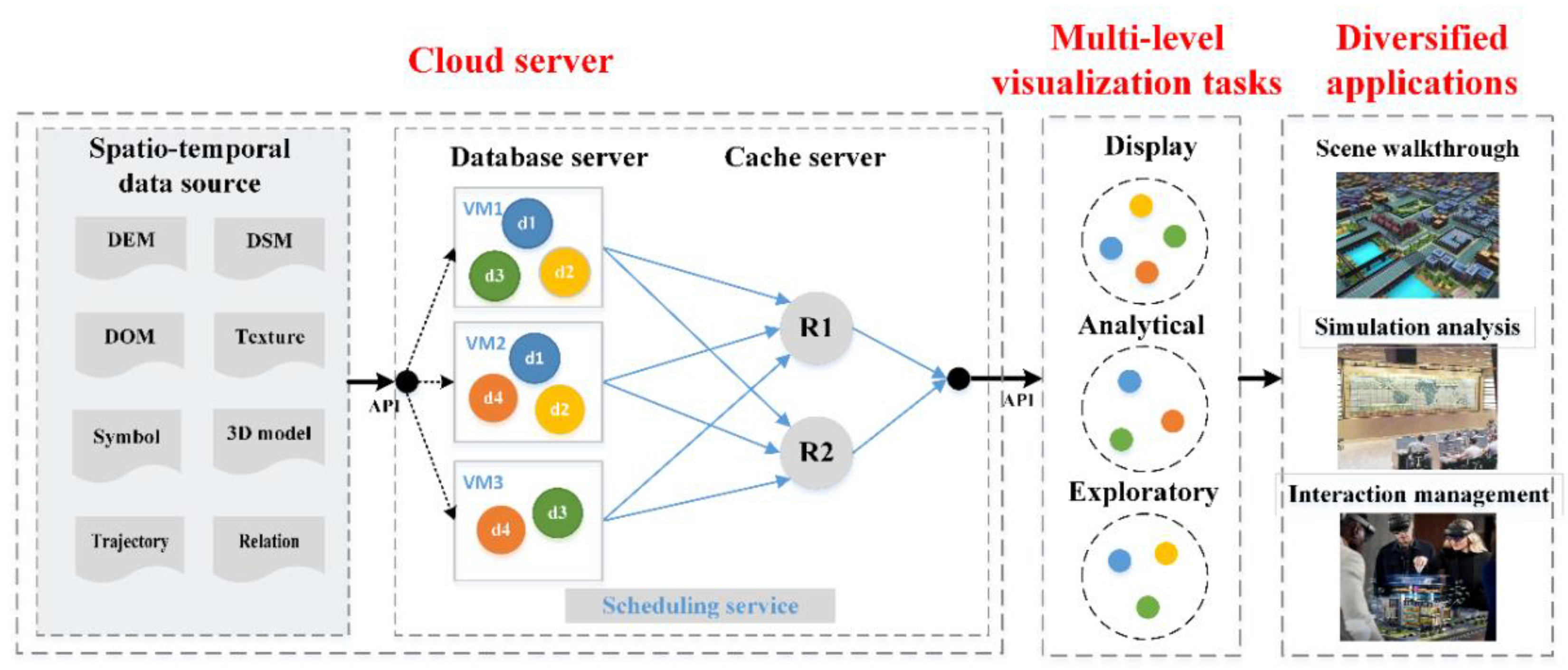
• Defined a multilevel visualization task and its data preference and designed framework of spatiotemporal data scheduling according to the structure of spatiotemporal data storage and scheduling in a cloud environment.
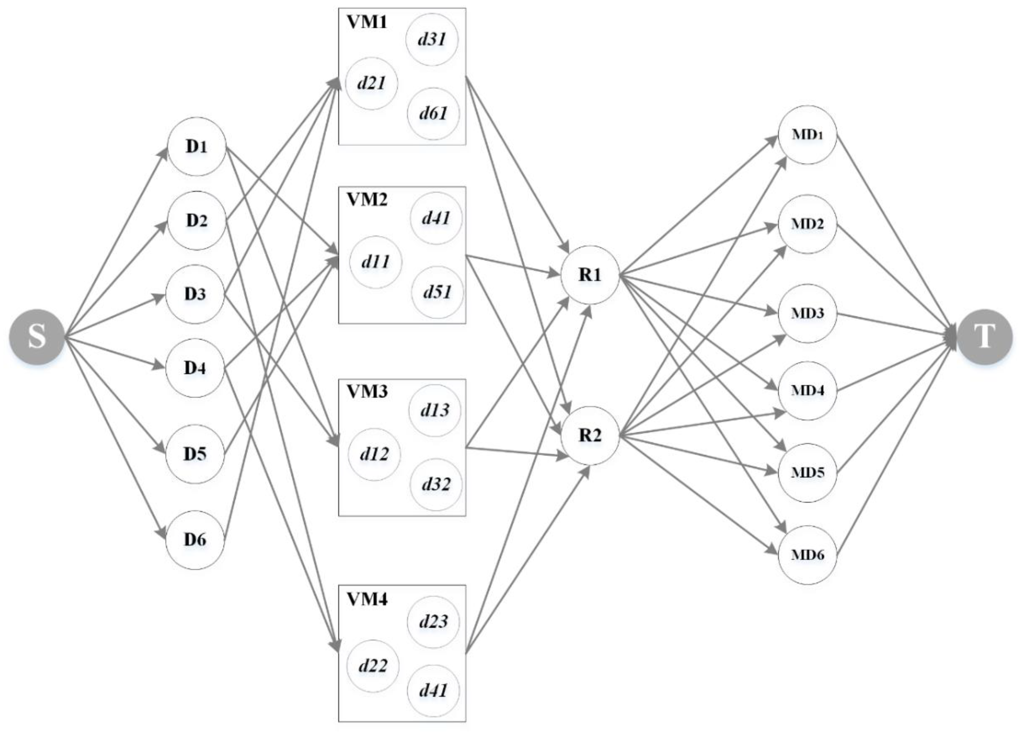
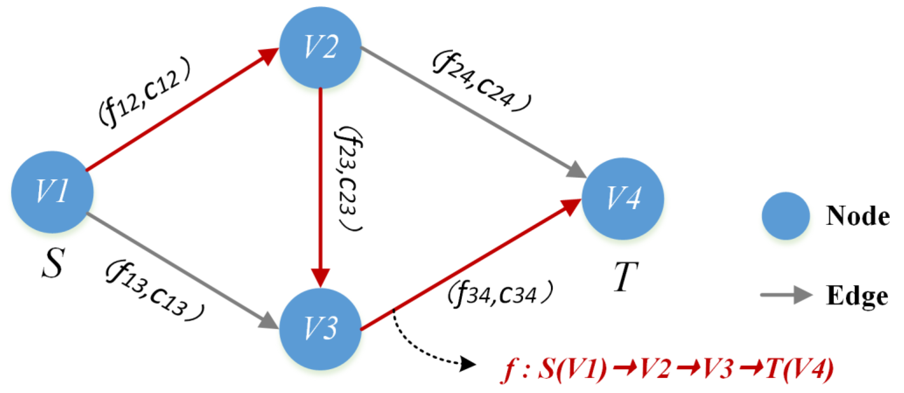
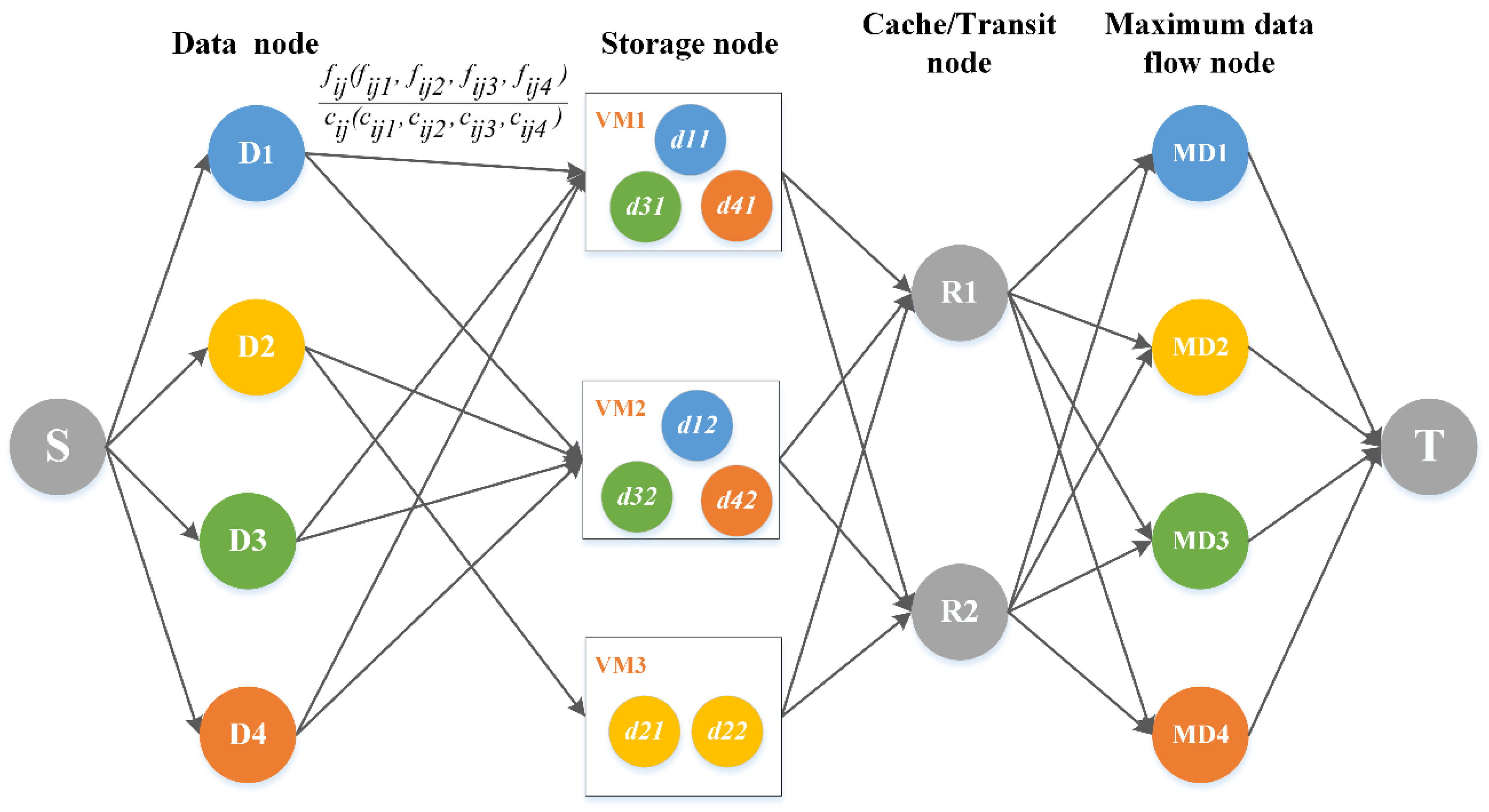
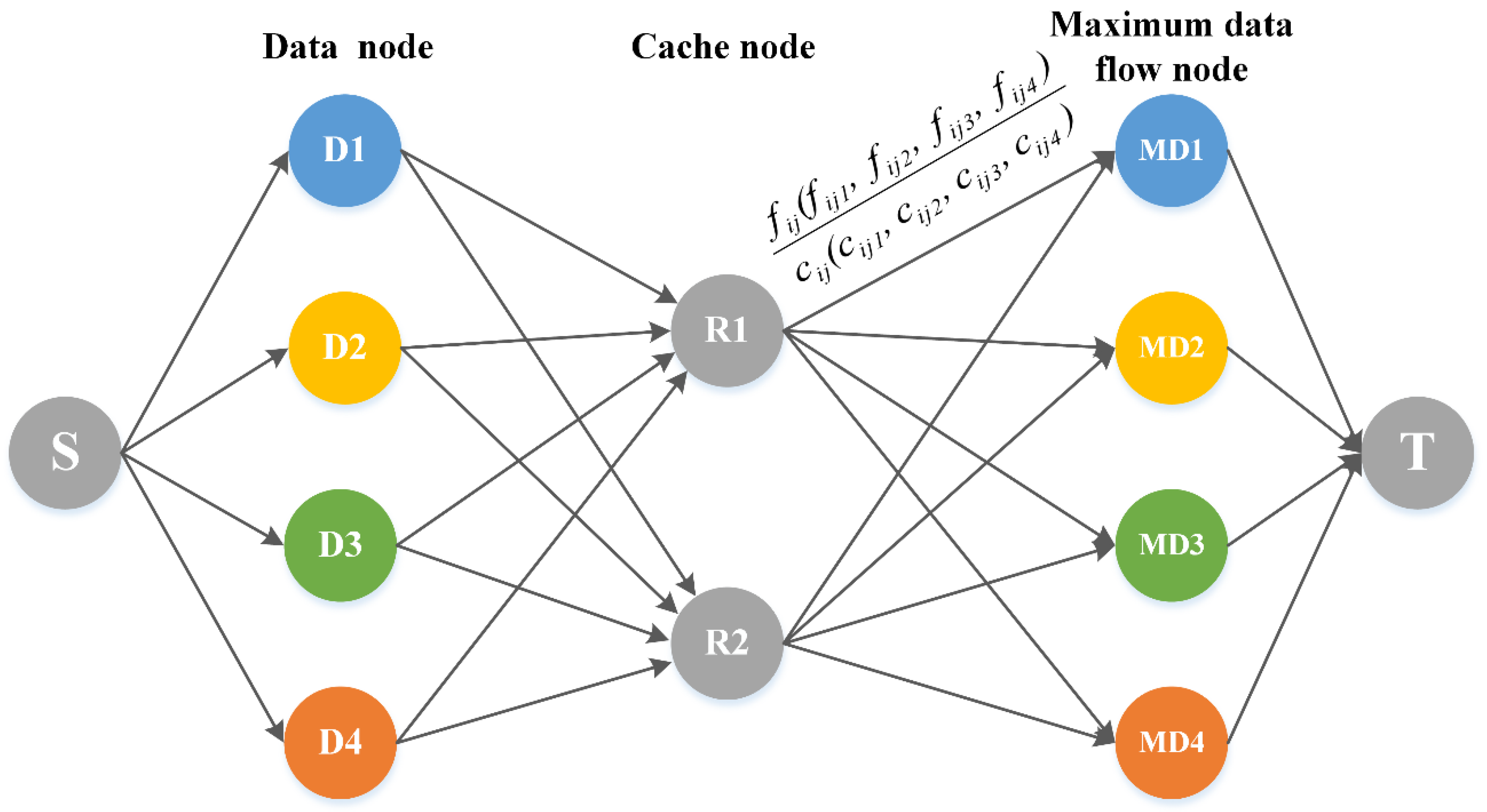
• Mapping the network topology of data resource scheduling to the maximum flow model and constructed a maximum flow scheduling model of spatiotemporal data can clearly quantify the ability of multisource and multigranular spatiotemporal data services.
• Designed two task-driven dynamic adjustment methods of maximum flow model parameters: cache node and storage node capacity allocation. This method can control the multitype spatiotemporal data flow size while maintaining the optimization of global data flow, and flexibly adapt to the needs of tasks under limited hardware resources in the cloud environment.

The rest of this paper is organized as follows: Section 2 presents the design of the spatiotemporal data scheduling framework. Section 3 shows the construction of a spatiotemporal data scheduling model based on maximum flow. Section 4 describes the task-driven maximum flow adjustment method for data flow optimization. A prototype system for spatiotemporal data scheduling and a user-friendly web-based parameter adjustment interface are developed, and an experimental analysis is implemented in Section 5. Finally, the conclusion and discussion are addressed in Section 6.

2. Spatiotemporal Data Scheduling Framework for Multilevel Visualization Tasks

The spatiotemporal data scheduling method for multilevel visualization tasks needs to consider not only the characteristics of spatiotemporal data but also the different scheduling requirements of multilevel visualization tasks in detail. To construct an efficient spatiotemporal data scheduling mechanism that adapts to complex changes in 3D scene visualization tasks, Section 2.1 first analyses the scheduling requirements of multilevel visualization tasks. Then, Section 2.2 designs a spatiotemporal data scheduling framework for multilevel visualization tasks.

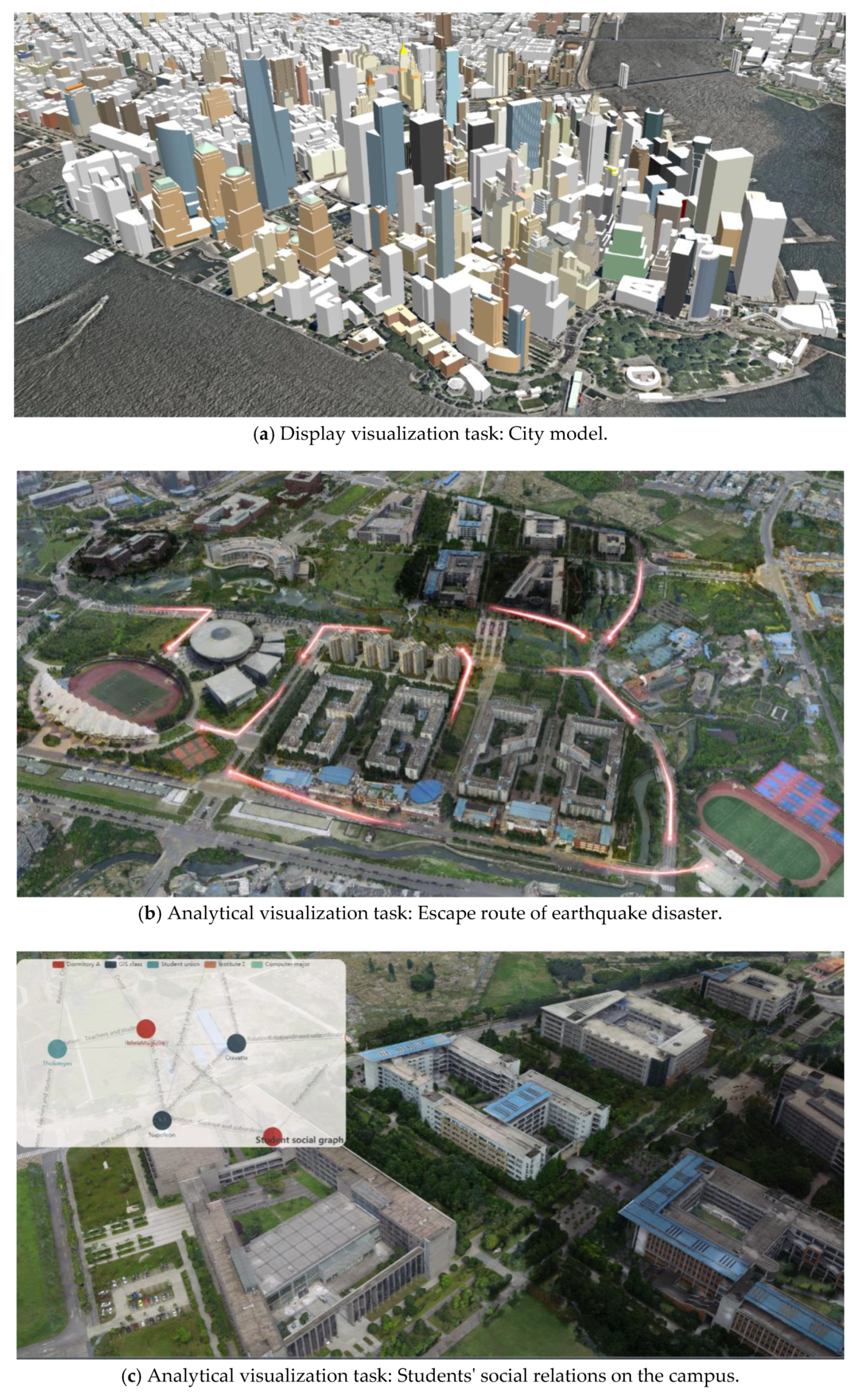
2.1. Multilevel Visualization Tasks and Data Preferences

Multimodal spatiotemporal data are driven by the requirements of multilevel visualization tasks. The visualization of data and the construction of scenes have become important means to display, recognize and control cyber-physical-social space. In the application of spatiotemporal data visualization, large-scale diversified clients access the spatiotemporal data visualization service in real time, and these clients have different levels of visualization tasks, resulting in different requirements for spatiotemporal data content. According to the scale of data rendering, fineness of 3D scene construction and application objectives, three kinds of visualization tasks corresponding to different scene content and data scheduling preferences are summarized below [44,45,46,47].

Display visualization task: This task focuses on the adaptive representation of spatiotemporal data in discrete–continuous, dynamic–static, realistic–abstract and fine–coarse scenes, as well as collaborative visualization that is highly integrated with real scenes. For example, urban patterns (terrain, buildings and roads) change dynamically with time, and although the scope of view and elements can be predicted, the data volume is large, so the database query output is the main task. Scheduling aims at efficient I/O and high-performance real-time scene rendering.

Analytical visualization task: This task highlights the hidden features and correlation information in the spatiotemporal data obtained by complex computational analysis. Typical applications include dynamic visualization of real-time calculations, near real-time simulation results, and integration visualization of symbolization and real scenes. This task is mainly based on data analysis and simulation calculations and needs the cooperation of scheduling methods to speed up the efficiency of the analysis process and the dynamic generation of results.

Exploratory visualization task: Through the exploratory adjustment operations of focusing, deformation and highlighting of specific objects in the augmented reality scene, the organic coupling of the data, the human brain, machine intelligence and application scenes is realized to support the visualization of deep association analysis such as hypothesis verification, knowledge induction and reasoning. For example, the multicomputer and multiuser collaborative interaction in a complex environment is mainly based on the fact interaction, focusing on the interactive analysis chain and the real-time visualization, while integrating the real-time dynamic analysis results and interactive content. Therefore, higher requirements are put forward for the scheduling of spatiotemporal data.

2.2. Spatiotemporal Data Scheduling Framework

As shown in Figure 1, the spatiotemporal data scheduling framework consists of three parts: cloud server, multilevel visualization tasks and diversified applications.

In Figure 1, three kinds of real-time visualization applications are listed: Scene walkthrough, Simulation analysis and Interaction management. The data requirements and application objectives of diversified visualization applications eventually form a large number of visualization tasks, which are divided into three categories according to the connotation of tasks, as described in the previous Section 2.1. Different levels of visualization tasks have different requirements for spatiotemporal data scheduling. Thus, the spatiotemporal data scheduling service in the cloud is required to dynamically meet the data access of diversified applications.

In Figure 1, the cloud server stores, caches, schedules and distributes the multisource and multigranularity raw data to the target visualization tasks, providing flexible and scalable spatiotemporal data services for diversified applications. After the raw data enter the cloud storage system, the data are deployed to different database servers through virtualization container and cluster technology. Then, according to the data access characteristics, the cache server switches the appropriate cache algorithm to cache the hotspot data and improve the efficiency of data services to share the backend database access pressure. When the system is running, through the allocation of storage resources and bandwidth resources of each database container type and the switching of the cache strategy, the dynamic allocation of spatiotemporal data flow is realized, multitype spatiotemporal data scheduling under multilevel visualization tasks is optimized, and the fine access requirements of multilevel visualization tasks are met.

3. Spatiotemporal Data Scheduling Model Based on Maximum Flow

This section describes the concept and structure of the proposed maximum flow scheduling (MFS) model for spatiotemporal data. Section 3.1 introduces the construction of the MFS model. Section 3.2 presents the initialization configuration of the node and edge capacity of the MFS model. Finally, a calculation method for the MFS model is introduced in Section 3.3.

3.1. Construction of Maximum Flow Model for Spatiotemporal Data Scheduling

The maximum flow model is a complex directed connected graph, which can be expressed as $\mathrm{G}=\left(\mathrm{V}, \mathrm{E}\right)$ with node set $\mathrm{V}$ and edge set E. $\mathrm{V}=\left\{v_i|i\in {\mathrm{Z}}^{+}\right\}$ is a collection of all nodes in the graph and $\mathrm{E}=\left\{\left(v_i,v_j\right)|i\in {\mathrm{Z}}^{+},j\in {\mathrm{Z}}^{+},i\ne j\right\}$ is a collection of all edges in the graph. In Figure 2, $v_1$ is the flow starting node of model $\mathrm{G}$, also known as source node $\mathrm{S}$, and $v_4$ is the flow convergence node of model $\mathrm{G}$, also known as sink node $\mathrm{T}$. Each edge has two parameters, $c_{ij}$ and $f_{ij}$, where $c_{ij}$ is the maximum flow that the edge can carry, also called the capacity, $f_{ij}$ is the actual transmission flow, and $f_{ij}\le c_{ij}$. Every node except S and T in model G obeys the principle of conservation of input and output flow, which can be expressed as $f^{+}\left(v_i\right)=f^{-}\left(v_i\right)$ ($f^{+}$ is the input flow into node $v_i$, $f^{-}$ is the output flow from $v_i$). A feasible flow $f$. in model $\mathrm{G}$ represents the amount of flow passing from node $\mathrm{S}$ to node $\mathrm{T}$. The maximum amount of feasible flows $f_{max}$ is called the maximum flow. The spatiotemporal data transmission network topology (in Figure 1) can be mapped to the maximum flow model, in which the server or cache server is mapped to model node V, which has two attributes: data type and data volume. The network connection is mapped to model edge E, which has bandwidth-limited attributes for each type of data.

The core concept of the maximum flow model is flow conservation, but a data copy can continuously provide data services. Therefore, this paper obtains an abstract transformation of the server-side spatiotemporal data scheduling framework (shown in Figure 1) and adds the corresponding auxiliary nodes for the MFS model (Figure 3). Through this transformation, the flow conservation of each spatiotemporal data scheduling step is realized, which conforms to the maximum flow model, and the service capacity of each spatiotemporal data set can be calculated. The nodes from left to right are source node S, data nodes D, storage nodes d, cache/transit data R, maximum data flow node MD and sink node T in Figure 3. The source node S in the model represents the spatiotemporal data source, and the sink node T represents the multilevel visualization task. To map the multitype data scheduling topology directly to the maximum flow model, some auxiliary data nodes $D$ and maximum data flow nodes $MD$ are added. Among them, $D=\left\{D_k|k=1,2,3,\dots q\right\}$ represents the resource set of each spatiotemporal data type. $MD=\left\{M{D}_k|k=1,2,3,\dots ,q\right\}$ represents the maximum flow of each spatiotemporal data type $D_k$, also known as the maximum data service capability that the system can provide to the visualization tasks, which is obtained by solving the MFS model.

Moreover, storage nodes $d=\left\{d_{kn}|k=1,2,3,\dots q, n=1,2,3\dots ,p\right\}$, where k represents the type of data and n represents the number of replicas, are containerized databases that are allocated disc space to store spatiotemporal data of different types, granularities, and volumes in the virtual machine server VM. Cache nodes.

$R=\left\{R_M|M=1,2,3,\dots ,m\right\}$ are containerized in memory databases that can share the access pressure of the server-side database. Assume that under ideal conditions, all data requests miss in the cache, and the cache node is regarded as a transit node. The transit node also follows the rules for flow conservation and completely transfers data flow sent from the server to the MD node. The maximum flow of $D_k$ is recorded as $Z_1\left(M{D}_k\right)$. If there is a request hit in the cache, the data flow directly from the cache node to the $\mathrm{MD}$ node. If all requests hit in the cache, the maximum flow of $D_k$ is recorded as $Z_2\left(M{D}_k\right)$, and the MFS model in this case is as shown in Figure 4. However, in a practical state, the range of the maximum flow of $D_k$ must satisfy $Z\left(M{D}_k\right)\in \left(Z_1\left(M{D}_k\right),Z_2\left(M{D}_k\right)\right)$; thus, $Z_1\left(M{D}_k\right)$ is called the lower limit, and $Z_2\left(M{D}_k\right)$ is called the upper limit.

3.2. Initialization Configuration of Node and Edge Capacity

Virtualization container technology is highly portable, lightweight, and more secure, which can improve the fault tolerance of data storage and result in high availability. Therefore, this paper uses virtualization container technology to deploy database clusters in different servers. Unbalanced data placement in a server leads to an excessive data transmission time and reduces the data throughput of the cloud data service. Therefore, this paper adopts a multireplica strategy to deploy multiple replicas of the same data on different servers. In addition, we need to consider the dependency between the data. For example, if both data $D_k$ and $D_{k+i}$ need to be scheduled in the scene construction phase, they can be considered highly dependent and not suitable for placement in the same server; otherwise, they will cause server resource competition.

Two types of nodes in the model enable the storage of spatiotemporal data: storage node d and cache node $R$. Among them, the initialization configuration of d determines how many replicas and in which server to place the data $D_k$. The initialization configuration of $R$ selects the initial cache replacement algorithm to store hotspot data. Generally, the initialization configurations of both $d$ and $R$ rely on expert experience. In Figure 3 and Figure 4, the capacity and flow of the edge in the MFS model of each data type are expressed as $f_{ij}\left(f_{ij1},\dots ,f_{ijk},\dots ,f_{ijq}\right)/c_{ij}\left(c_{ij1},\dots ,c_{ijk},\dots ,c_{ijq}\right)$, where $f_{ij} \mathrm{is} \mathrm{the} \mathrm{total} \mathrm{data} \mathrm{flow}$ of the edge and $f_{ijk}$ is the flow of each $D_k$, $f_{ij}={\sum }_{k=1}^q{f}_{ijk}$. $c_{ij}$ is the total transmission capacity of the edge, and $c_{ijk}$ is the transmission capacity of each $D_k$, $c_{ij}={\sum }_{k=1}^q{c}_{ijk}$. The initialization configuration of the edge capacity is described in detail below:

The $\mathrm{edge}\left(D_k,VM\right)$ in Figure 3 is the connection between the auxiliary data nodes and the storage node, and the $\mathrm{edge} \left(D_k,R_M\right)$ in Figure 4 is the connection between the auxiliary data nodes and the cache node. $c_{ij}$ of $\mathrm{edge}\left(D_k,VM\right)$ and $\mathrm{edge} \left(D_k,R_M\right)$ is defined as the amount of data actually deployed on the server $VM$ and cache server R, respectively, and $c_{ijk}$ is the amount of each type of data actually deployed.

The data transmission capacity of $\mathrm{edge} \left(VM,R_M\right)$ in Figure 3 between the storage node and the cache node is obviously affected by the bandwidth and the amount of data stored. In Equation (1), ${\mathrm{b}}_{\left(VM, R_M\right)}$ is the network bandwidth between the two nodes $VM$ and $R_M, dataSize\left(d_{kn}\right)$ represents the data amount of storage node $d_{kn}$, α is a constant calculated from the bandwidth and the amount of data, and t is the transfer time. Under the same network bandwidth, the larger amount of data stored in server $VM$, the longer time taken to complete all data transmission. Therefore, this paper defines $c_{ij}$ of $\mathrm{edge}\left(VM,R_M\right)$ in this way, which is inversely proportional to the amount of data stored by the server $VM$, and $c_{ijk}$ of $\mathrm{edge}\left(VM,R_M\right)$ is calculated by allocating the maximum transmission capacity $c_{ij}$ according to the ratio of $D_k$ to the total data amount, as shown in Equation (2).

$${\mathrm{c}}_{ij}={\mathrm{b}}_{\left(VM, R_M\right)}/\sum _{k=1}^q\sum _{n=1}^{p}dataSize\left(d_{kn}\right)\propto \mathsf{\alpha }\times \frac{1}{t}$$

(1)

$$c_{ijk}=\sum _{n=1}^{p}dataSize\left(d_{kn}\right)/\sum _{k=1}^q\sum _{n=1}^{p}dataSize\left(d_{kn}\right) \ast c_{ij}$$

(2)

The data transmission capacity of $\mathrm{edge}\left(R_M, M{D}_k\right)$ is also affected by the bandwidth and the amount of data stored. Setting the bandwidth between the nodes $R_M$ and $M{D}_k$ as ${\mathrm{b}}_{\left(R_M, M{D}_k\right)}$, the cache blocks $r_{ }=\left\{r_{kl}|k=1,2,3\dots ,q, l=1,2,3,\dots ,y\right\}$ of multitype spatiotemporal data are stored in the cache node $R$, where $r_{kl}$ is the l-th cache block of $D_k$. Similar to the definition of $c_{ijk}$ of $\mathrm{edge}\left(VM, R_M\right)$, $c_{ijk}$ of $\mathrm{edge}\left(R_M, M{D}_k\right)$ is defined as shown in Equation (3).

$$c_{ijk}=\sum _{l=1}^{y}dataSize\left(r_{kl}\right)/\sum _{k=1}^q\sum _{l=1}^{y}dataSize\left(r_{kl}\right) \ast c_{ij}$$

(3)

The connection between the auxiliary maximum data flow node and sink node is recorded as $\mathrm{edge}\left(M{D}_k,\mathrm{T}\right)$, which is the supply path of each type of data flow to the client side in the scheduling service. The ${\mathrm{c}}_{ijk}$ of $\mathrm{edge}\left(M{D}_k,\mathrm{T}\right)$ is the maximum flow of $D_k$, calculated by the MFS model.

Furthermore, $\mathrm{edge}\left(v_i,v_j\right)$ is necessary to comply with two constraints in the MFS model.

Capacity limit: necessary to meet the total flow limit of all types of data; the capacity limit of each type of data $D_k$,$0\le {\sum }_{k=1}^q{f}_{ijk}\le c_{ij}$ and $f_{ijk}\le c_{ijk}$, k = 1,2,3, …, q;

Flow conservation: all nodes must follow the flow conservation rules, including both the total data flow to be conserved and each type of data flow to be conserved, ${\sum }_{k=1}^q{f}^{+}\left(v_i\right)={\sum }_{k=1}^q{f}^{-}\left(v_i\right)$ and $f^{+}\left(v_i\right)=f^{-}\left(v_i\right)$, k = 1,2,3, …, q;

Based on the above analyses, the objective function and constraints of the MFS model for spatiotemporal data are shown in Equations (4) and (5), where ${\sum }_k^q{f}_{ijk}$ is the maximum amount of feasible flows of all data in the MFS model.

$${\sum }_{k=1}^{q}Z\left(M{D}_k\right)={\sum }_{k=1}^q{f}_{ijk}, k=1,2,3\dots q \left(\mathrm{Objective} \mathrm{function}\right)$$

(4)

$$s.t.\{\begin{array}{cc}{Z}_1\left(M{D}_k\right)<Z\left(M{D}_k\right)<Z_2\left(M{D}_k\right)\hfill & (\mathrm{range} \mathrm{of} \mathrm{the} \mathrm{maximum} \mathrm{flow})\\ \hspace{1em}0\le {\displaystyle \sum _{k=1}^q}{f}_{ijk}\le c_{ij}\hfill & (\mathrm{total} \mathrm{capacity} \mathrm{limit})\\ \hspace{1em} f_{ijk}\le c_{ijk}\hfill & \left(\mathrm{each} \mathrm{type} \mathrm{of} \mathrm{data} \mathrm{flow} \mathrm{capacity} \mathrm{limit}\right)\\ \hspace{1em} {\displaystyle \sum _{k=1}^q}{f}^{+}\left(v_i\right)={\displaystyle \sum _{k=1}^q}{f}^{-}\left(v_i\right)\hfill & \left(\mathrm{total} \mathrm{flow} \mathrm{conservation}\right)\\ \hspace{1em} f^{+}\left(v_i\right)=f^{-}\left(v_i\right)\hfill & \left(\mathrm{each} \mathrm{type} \mathrm{of} \mathrm{data} \mathrm{flow} \mathrm{conservation}\right)\end{array}$$

(5)

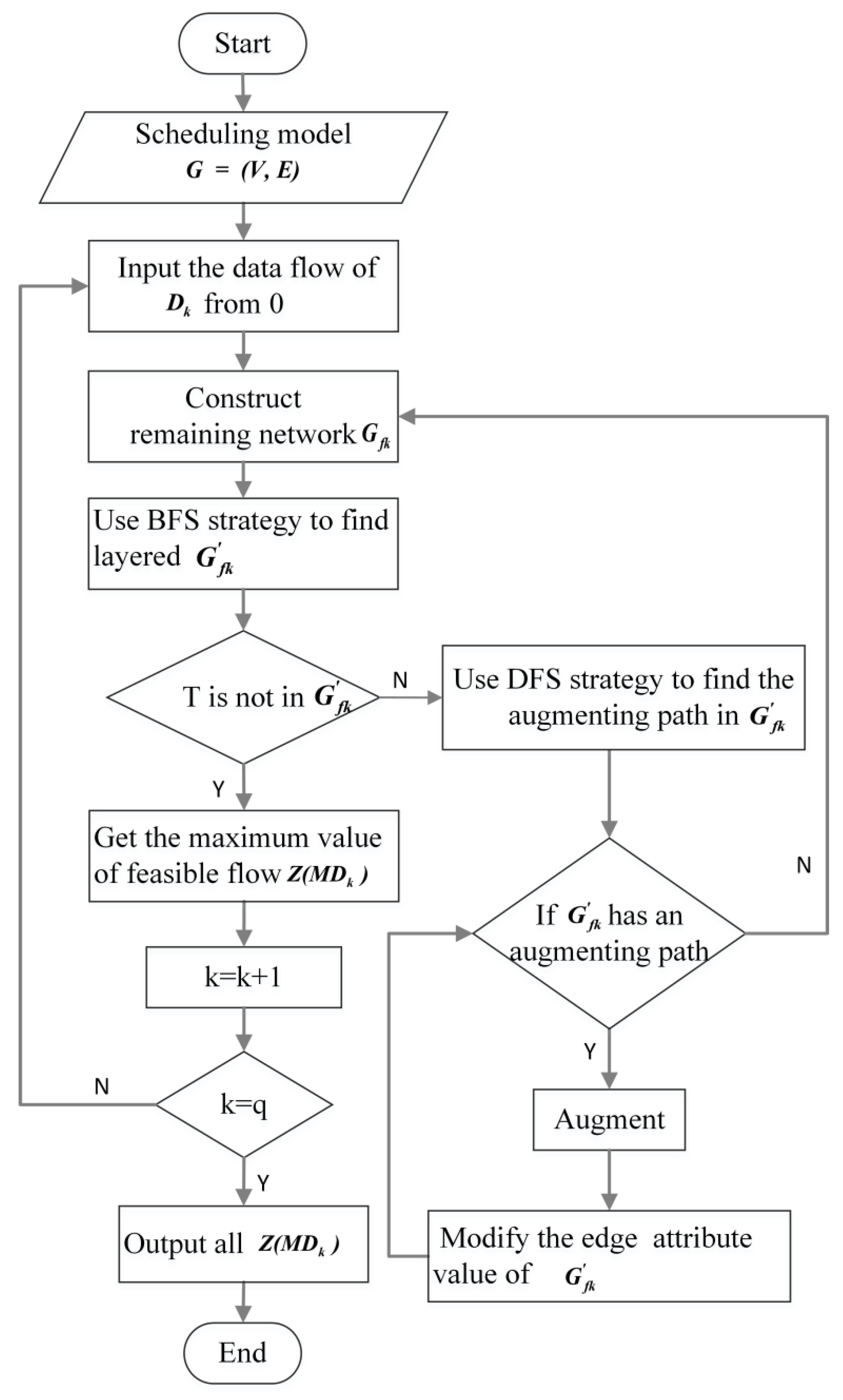
3.3. Maximum Flow Algorithm

The goal of spatiotemporal data flow global optimization is to maximize the feasible flow of all data in the model. After initializing the flow model, the lower and upper limits of maximum data flow $Z_1\left(M{D}_k\right),Z_2\left(M{D}_k\right)$ are solved according to the improved maximum flow algorithm Dinic [48], which can efficiently solve the maximum flow value of multitype data. The core idea of the algorithm is to use the BFS (breadth-first-search) strategy to layer and traverse the nodes of the remaining network $G_{fk}^{}$ of model G, thus obtaining the layered residual network $G_{fk}^{\prime }$, and to use DFS (depth-first-search) to find the augmenting path and value of $G_{fk}^{\prime }$ [49]. Augmenting path is a path from node s to node T in the model G = (V, E), along which more flow can be transmitted [50]. The detailed steps of the Dinic algorithm are as follows, and the algorithm flow chart is shown in Figure 5.

• Inputting the data flow of $D_k$ from 0 in the model $\mathrm{G}=\left(\mathrm{V},\mathrm{E}\right)$;
• Construct the remaining network $G_{fk}^{}$ of the model $\mathrm{G}=\left(\mathrm{V},\mathrm{E}\right)$ and use the BFS strategy to find the layered residual network $G_{fk}^{\prime }$ of the scheduling model; if the sink node is not in $G_{fk}^{\prime }$, go to (6);
• Use the DFS strategy to find the augmenting path. If $G_{fk}^{\prime }$ has an augmenting path from source node S to sink node T, go to (4); if not, go to (5);
• According to the found augmenting path and the augmenting value, augment and modify the directed edge attribute of the layered residual network $G_{fk}^{\prime }$, then go to (3);
• $G_{fk}^{\prime }$ has no augmenting path available; go to (2);
• The resulting feasible flow is the maximum flow $Z\left(M{D}_k\right)$ of $D_k$;
• To start increasing the flow of $D_{k+1}$, repeat steps (2) through (6) until k = q.

Finally, the lower and upper limits of the maximum data flow are obtained according to Equation (6).

$$\begin{gathered} Z_1\left(M{D}_k\right)=\left\{Z_1\left(M{D}_1\right),Z_1\left(M{D}_2\right),\dots ,Z_1\left(M{D}_k\right),\dots |k=1,2,3,\dots ,q\right\} \\ {Z}_2\left(M{D}_k\right)=\left\{Z_2\left(M{D}_1\right),Z_2\left(M{D}_2\right),\dots ,Z_2\left(M{D}_k\right),\dots |k=1,2,3,\dots ,q\right\} \\ Z\left(M{D}_k\right)\in \left(Z_1\left(M{D}_k\right),Z_2\left(M{D}_k\right)\right) \end{gathered}$$

(6)

4. Task-Driven Maximum Flow Allocation Method for Spatiotemporal Data

In the cloud service, by adjusting the parameters of the maximum flow model to change the lower $Z_1\left(M{D}_k\right)$ and upper $Z_2\left(M{D}_k\right)$ limit of a certain spatiotemporal data, the overall maximum flow of all data service can be maintained to dynamically meet the different access requirements of multilevel visualization tasks. Section 4.1 introduces the flow adjustment method based on the cache node, and Section 4.2 introduces the flow adjustment method based on the storage node.

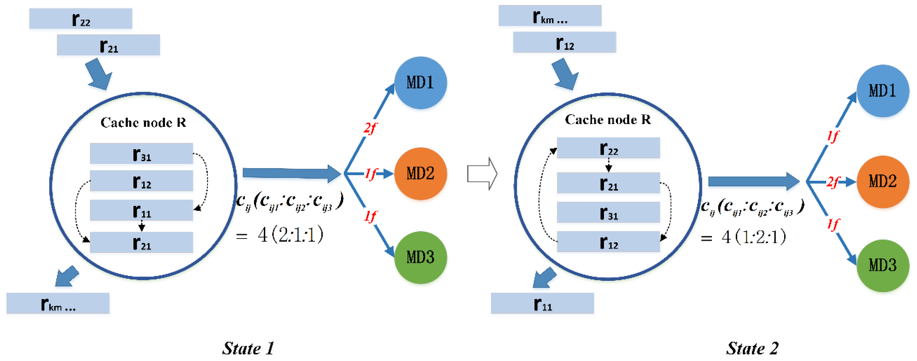
4.1. Capacity Allocation of Cache Node

The cache achieves fast data reading and high performance compared with the external database container, which is used to improve the data access ability of the system. The transmission capacity allocation of the cache node can be changed by selecting a specific cache algorithm and policy. Over time, more data types are added to the cache node; if the cache node is full, the adaptive replacement algorithm is used to eliminate the cold data and prepare storage space for new data. Since different levels of visualization tasks have an obvious preference for spatiotemporal data, if the current cache node cannot meet the burst data request in the running state, the cache node algorithm can be temporarily switched to change the content of the data stored in the cache node to adapt to the needs of dynamic changes. Therefore, a task-driven hybrid cache algorithm is designed to improve the data flow based on the cache size, hit rate, and access frequency. For example, if the client task has no obvious data preference, the LRU or LFU replacement algorithm considering the LOD can be used. On the basis of LRU or LFU, high-LOD objects can be eliminated first, which can not only minimize the amount of cached data but also ensure that as many objects are retained in the cache as possible, significantly improving the hit rate of the client memory cache. If the client task has an obvious data preference, the active preloading strategy, instead of on-demand loading, can be adopted, in which the target data are first cached in the memory and then the data service ability is improved. At the same time, due to the spatial proximity of spatial object access, the objects in close spatial proximity have similar access frequencies; hence, the cache replacement algorithm based on spatial proximity can be added.

As shown in Figure 6, the cache algorithm adjusts the state of the data configuration in the cache node, and the change in the amount of data causes the transmission capacity of the edge to change. As described in Section 3.2, when the proportion of hotspot data blocks increases in the cache node, its maximum transmission capacity $c_{ijk}$ also increases proportionally. In summary, the task-driven hybrid caching algorithm plays an important role in increasing the hotspot data flow transmission capacity in the scheduling service.

4.2. Capacity Allocation of Storage Node

When the data access preferences change with high-concurrency tasks, by changing the hybrid caching algorithm, the flow of the preference data can be improved, but the adjustment of the hybrid cache algorithm achieves only the purpose of increasing the preference data upper limit of the maximum flow $Z_2\left(M{D}_k\right)$; the lower limit of the flow is still not changed. The practical data flow can still be near the lower limit. Therefore, another way to comprehensively increase the preference data maximum flow is by adjusting the edge capacity allocation of the underlying server where the storage node is located.

According to the data access preferences of visualization tasks, these two kinds of adjustment strategies can change the flow size of each type of spatiotemporal data to meet the task requirements. Among them, the hybrid cache node algorithm adjustment method makes changes faster and is more flexible, while the server connection edge capacity allocation method can accurately allocate the maximum flow of the spatiotemporal data and improves the flow bandwidth of spatiotemporal data from the bottom, which is more effective. In an actual project, the spatiotemporal data flow adjustment strategy can be selected according to the task changes to meet the data flow requirements of multilevel visualization tasks at the lowest cost.

5. Experimental Analysis

To verify the effectiveness of the proposed MFS method in task-driven spatiotemporal data visualization, we designed spatiotemporal data scheduling experiments corresponding to three visualization task levels, with six types of typical spatiotemporal data, including DEM, Building model, DSM, Trajectory, Relation and Pipeline data, which are described in detail in

Table 1. Description of experimental datasets.

Visualization Task	${\mathit{D}}_{\mathit{k}}$	Data Type	Data Size (GB)	Number of Containers
Display	$D_1$	DEM	5.0	3
	$D_2$	Building model	4.3	3
Analytical	$D_3$	DSM	3.0	2
	$D_4$	Trajectory	3.1	2
	$D_5$	Relation	1.6	1
Exploratory	$D_6$	Pipeline	1.3	1

. Compared the MFS method with the two most important strategies, namely, first come first serve (FCFS) [41] and the priority scheduling algorithm (PSA) [51], by simulating and analyzing the actual data throughput changes, and verified the feasibility of the MFS method.

5.1. Experimental Environment and Data

The spatiotemporal data scheduling experiment is implemented with Java v. 1.8, and a web-based interface for parameter configuration and data flow monitoring is developed. The storage nodes are implemented by the container-based MongoDB v. 4.0.12, and the cache nodes are implemented by the container-based Redis v. 5.0.5. The whole experimental system is deployed on seven virtual machines, each of which is installed with the CentOS 7 operating system and has a dual-core processor, 4 GB of RAM and a 50 GB hard disk size. Four of the VMs are used as storage nodes, two as cache nodes and one as a data scheduling service.

Six kinds of typical spatiotemporal data are prepared in the experiment, as shown in Table 1, in which display scene visualization tasks are based on the DEM and building model, analytical scene visualization tasks are based on the DSM and trajectory and relation data [52,53], and exploratory scene visualization tasks use pipeline data. To evaluate the accuracy of our proposed MFS method, we used open datasets (Building model datasets) for NYC (http://maps.nyc.gov/download/3dmodel/DA_WISE_GML.zip). Typical application scenes of three types of visualization tasks are shown in Figure 7. Figure 7a describes the city model, which belongs to the display visualization task; Figure 7b obtains the best path of earthquake escape through simulation analysis, and Figure 7c presents the knowledge representation of social relationships in the campus, which both belong to the analytical visualization task. Figure 7d describes the precise troubleshooting of the pipeline fault in the interactive augmented reality environment, which belongs to the exploratory visualization task.

5.2. Experimental Results and Analysis

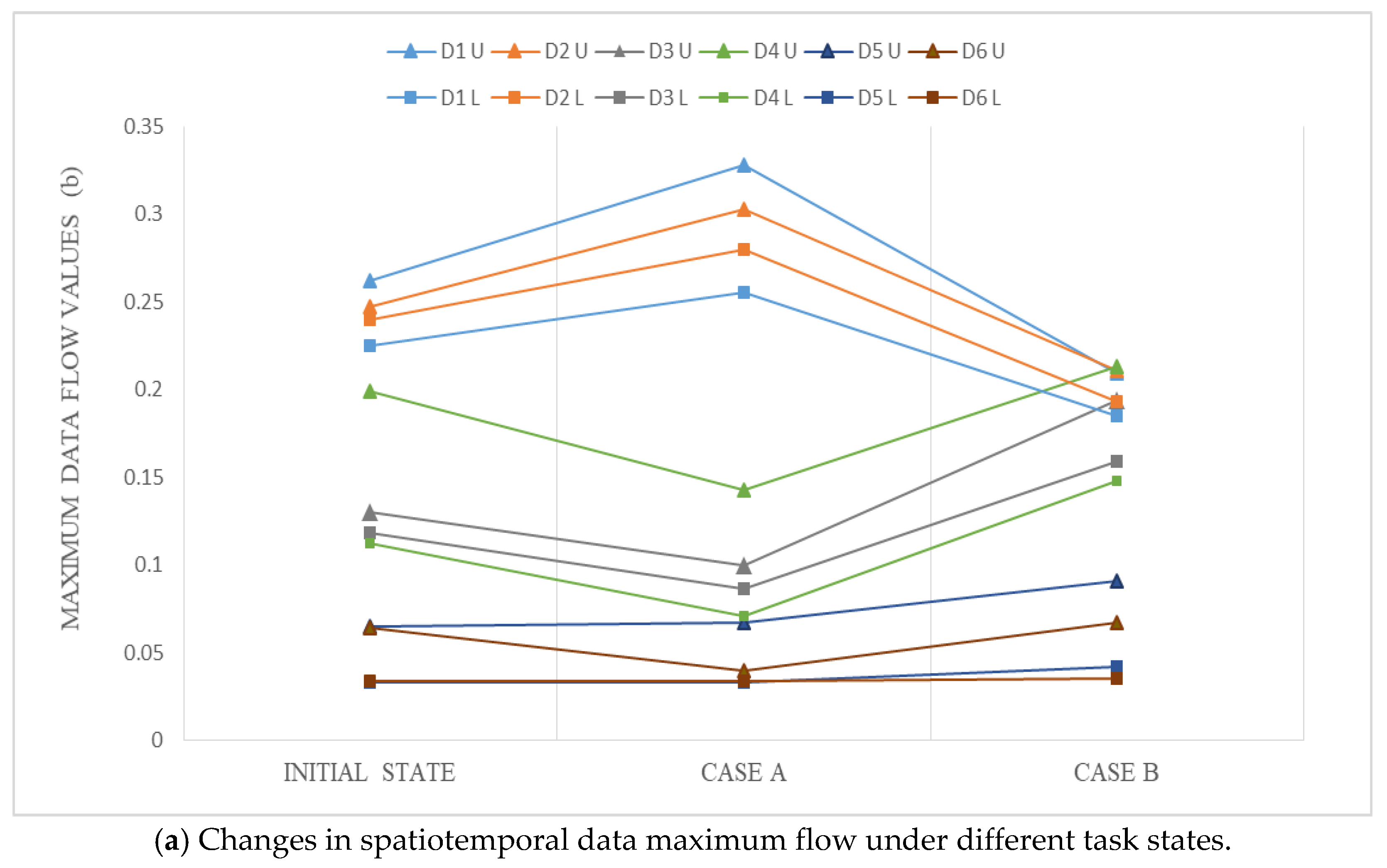
5.2.1. Data Maximum Flow Calculation of the Initial State

According to the requirements of multilevel visualization tasks, the spatiotemporal data storage service is built, and the scheduling parameters are configured. The MFS model of the experimental spatiotemporal data is constructed in Figure 8. The node configuration status and data transmission capacity of each edge are shown in

Table 2. Node configuration and data transmission capacity.

Node Number	Node Data Size (GB) $({\mathit{D}}_1$$, {\mathit{D}}_2$$, {\mathit{D}}_3$$, {\mathit{D}}_4$$, {\mathit{D}}_5$$, {\mathit{D}}_6)$	Capacity $({\mathit{c}}_{\mathit{i}\mathit{j}1},{\mathit{c}}_{\mathit{i}\mathit{j}2},{\mathit{c}}_{\mathit{i}\mathit{j}3},{\mathit{c}}_{\mathit{i}\mathit{j}4},{\mathit{c}}_{\mathit{i}\mathit{j}5},{\mathit{c}}_{\mathit{i}\mathit{j}6})\mathbf{b}$
${\mathrm{VM}}_1$	(0, 4.3, 3.0, 0, 0, 1.3)	(0, 0.058, 0.041, 0, 0, 0.017)b
${\mathrm{VM}}_2$	(5.0, 0, 0, 3.1, 1.6, 0)	(0.053, 0, 0, 0.034, 0.017, 0)b
${\mathrm{VM}}_3$	(10.0, 0, 3.0, 0, 0, 0)	(0.059, 0, 0.018, 0, 0, 0)b
${\mathrm{VM}}_4$	(0, 8.6, 0, 3.1, 0, 0)	(0, 0.062, 0, 0.023, 0, 0)b
${\mathrm{R}}_1$	(0.6, 0.5, 0.25, 0.4, 0.15, 0.1)	(0.143, 0.129, 0.057, 0.094, 0.036, 0.026)b
${\mathrm{R}}_2$	(0.5, 0.5, 0.3, 0.45, 0.125, 0.125)	(0.119, 0.118, 0.073, 0.106, 0.029, 0.039)b

, which are calculated by Equations (1)–(3), where ${\mathrm{b}}_{\left(VM,R_M\right)}={\mathrm{b}}_{\left(R_M, M{D}_k\right)}=\mathrm{b}$. The lower and upper limits of each type of spatiotemporal data $Z_1\left(M{D}_k\right)$ and $Z_2\left(M{D}_k\right)$ under the initial state can be obtained by the Dinic algorithm, as shown in

Table 3. Maximum data flow values under the initial state.

${\mathit{D}}_{\mathbf{k}}$	${\mathit{Z}}_1\left(\mathit{M}{\mathit{D}}_{\mathit{k}}\right)$	${\mathit{Z}}_2\left(\mathit{M}{\mathit{D}}_{\mathit{k}}\right)$
$D_1$	0.225b	0.262b
$D_2$	0.240b	0.247b
$D_3$	0.118b	0.130b
$D_4$	0.112b	0.199b
$D_5$	0.033b	0.065b
$D_6$	0.034b	0.064b

.

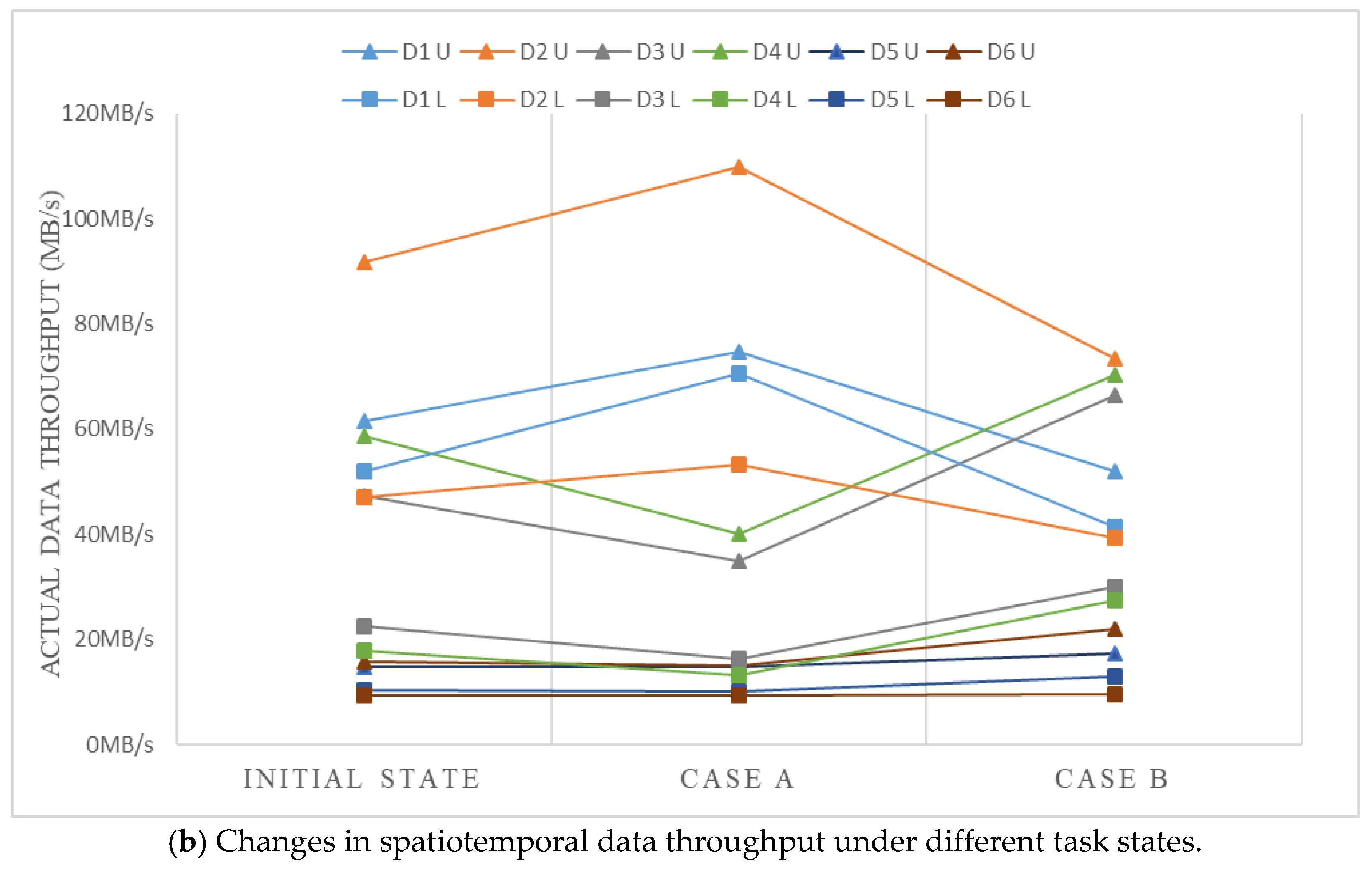
5.2.2. MFS Model Adjustment

The web-based spatiotemporal data maximum flow management interface is shown in Figure 9, and the chart elements are implemented with Echarts [54]. The management interface can be used to adjust capacity parameters to meet the different requirements of different levels of visualization tasks for spatiotemporal data. By dragging the server and cache slider, the capacity parameters of the edge are changed, resulting in a change in the service ability of each spatiotemporal data type in the cloud environment. By simulating the requests for three types of visualization tasks as described in Figure 7: Display visualization task: City model; Analytical visualization task: Escape route of earthquake disaster and Students’ social relations on the campus; Exploratory visualization task: Pipeline troubleshooting. The actual throughput of each data type can be monitored in real time, as shown in the lower-left chart. In addition, under the current parameter configurations, the upper- and lower-limit values of each type of spatiotemporal data calculated according to the method in this paper are shown in the lower right chart.

The test method used in the data scheduling experiment requests and schedules all spatiotemporal data through sequential traversal. In addition, the beginning part of each type of spatiotemporal data sequence is cached in the cache node. Therefore, during the experiment, the requests will be hit in memory and then will be processed through the backend server. Through this special test method, we can test the actual system data throughput when the MFS model is in the upper- and lower-limit states. Next, we verify the effectiveness of this method through two specific multilevel visualization task cases.

Case A: When a large number of display tasks are connected to the scheduling system, data access prefers $D_1$ and $D_2$, and the data service resource with a low access rate can be allocated to the data service with an intensive access rate to improve the system response speed and resource utilization. Therefore, the slider on the maximum flow management interface is dragged, the capacity parameters are adjusted and the service ability of $D_1$ and $D_2$ is improved. The upper limits $Z_2\left(M{D}_k\right)$ and the lower limits $Z_1\left(M{D}_k\right)$ of each type of spatiotemporal data under Case A can be obtained by the Dinic algorithm, as shown in

Table 4. Maximum data flow values under Case A (${\mathrm{b}}_{\left({VM}_{ },{ R}_M\right)}={\mathrm{b}}_{\left(R_M, M{D}_k\right)}=\mathrm{b})$.

${\mathit{D}}_{\mathbf{k}}$	${\mathit{Z}}_1\left(\mathit{M}{\mathit{D}}_{\mathit{k}}\right)$	${\mathit{Z}}_2\left(\mathit{M}{\mathit{D}}_{\mathit{k}}\right)$
$D_1$	0.255b	0.328b
$D_2$	0.280b	0.303b
$D_3$	0.086b	0.100b
$D_4$	0.071b	0.143b
$D_5$	0.033b	0.067b
$D_6$	0.034b	0.040b

. In contrast to Table 3, both the lower limits and upper limits of $D_1$ and $D_2$ are increased after adjustment. At the same time, the maximum flow value of $D_3$–$D_6$ is reduced.

With the change in model parameters, the actual data throughputs of $D_1$ and $D_2$ are also changed. The real-time throughput monitoring curves of $D_1$ and $D_2$ are shown in Figure 10. The former part of the throughput curves of $D_1$ and $D_2$ are higher because the data required by the task is hit in the cache node. At this time, the actual monitored throughput values correspond to the upper limit of the MFS model. While the latter part of the throughput values is reduced because the data required by the task are not hit, at this time, the actual monitored throughput values correspond to the lower limit of the MFS model. The data scheduling of $D_1$ is completed before that of $D_2$; thus, the subsequent actual monitored throughput of $D_1$ is reduced to 0.

In Figure 10a, the throughput of $D_1$ is initially maintained at 61.48 MB/s and then reduced to 51.96 MB/s, and the throughput of $D_2$ is initially maintained at 91.80 MB/s and then reduced to 46.95 MB/s under the initial state. After adjusting the model, the actual throughput values of $D_1$ and $D_2$ in Case A are as shown in Figure 10b. The throughput of $D_1$ is initially maintained at 74.61 MB/s and then reduced to 70.55 MB/s, and the throughput of $D_2$ is initially maintained at 109.8 MB/s and then reduced to 53.34 MB/s. By comparing Figure 10a,b, we find that the actual throughput of $D_1$ in the former part is increased by 21.36% and that the latter part is increased by 35.78%; the actual throughput of $D_2$ in the former part is increased by 19.61%, and the latter part is increased by 13.61%. In conclusion, by adjusting the parameters of the MFS model, the actual throughput of the display task preference data is improved, and the service ability of spatiotemporal data under the condition of an intensive display task is improved.

Case b: When a large number of analytical tasks are connected to the scheduling system, data access prefers $D_3$, $D_4$ and $D_5$. Similar to Case A, to improve the service ability of the system, more resources need to be allocated to $D_3$, $D_4$ and $D_5$. The upper limits and the lower limits of each type of spatiotemporal data under Case B can be obtained by the Dinic algorithm, as shown in

Table 5. Maximum data flow values under Case B (${\mathrm{b}}_{\left({VM}_{ },{ R}_M\right)}={\mathrm{b}}_{\left(R_M, M{D}_k\right)}=\mathrm{b})$.

${\mathit{D}}_{\mathit{k}}$	${\mathit{Z}}_1\left(\mathit{M}{\mathit{D}}_{\mathit{k}}\right)$	${\mathit{Z}}_2\left(\mathit{M}{\mathit{D}}_{\mathit{k}}\right)$
$D_1$	0.185b	0.209b
$D_2$	0.193b	0.211b
$D_3$	0.159b	0.194b
$D_4$	0.148b	0.213b
$D_5$	0.042b	0.091b
$D_6$	0.035b	0.067b

. In contrast to Table 3, the lower limits and upper limits of $D_3$, $D_4$ and $D_5$ are increased after adjusting; at the same time, the maximum flow values of $D_1$ and $D_2$ are reduced because fewer resources are allocated to them.

With the change in model parameters, the actual data throughputs of $D_3$, $D_4$ and $D_5$ are also changed. The real-time throughput monitoring curves of $D_3$, $D_4$ and $D_5$ are shown in Figure 11. The former part of the throughput curves is higher because the data required by the task are hit in the cache node. At this time, the actual monitored throughput values correspond to the upper limit of the MFS model. While the latter part of the throughput values is reduced because the data required by the task are not hit, at this time, the actual monitored throughput values correspond to the lower limit of the MFS model.

In Figure 11a, the throughput of $D_3$ is initially maintained at 47.38 MB/s and then reduced to 22.65 MB/s, the throughput of $D_4$ is initially maintained at 58.79 MB/s and then reduced to 17.79 MB/s, and the throughput of $D_5$ is initially maintained at 14.75 MB/s and then reduced to 10.28 MB/s under the initial state. After adjusting the model, the throughput of $D_3$ is initially maintained at 66.41 MB/s and then reduced to 30.01 MB/s, the throughput of $D_4$ is initially maintained at 70.30 MB/s and then reduced to 27.46 MB/s, and the throughput of $D_5$ is initially maintained at 17.44 MB/s and then reduced to 13.00 MB/s in Figure 11b. By comparing Figure 11a,b, the actual throughput of $D_3$ in the former part is increased by 40.16%, and that in the latter part is increased by 32.49%; the actual throughput of $D_4$ in the former part is increased by 19.58%, and that in the latter part is increased by 54.36%; and the actual throughput of $D_5$ in the former part is increased by 18.24%, while that in the latter part is increased by 26.46%. In conclusion, by adjusting the parameters of the MFS model, the actual throughput of analytical task preference data are improved, and the service ability of spatiotemporal data under the condition of an intensive analytical task is improved.

The adjustment of the parameters of each spatiotemporal data in the MFS model results in changes in the relevant data throughput. The relationship between them is shown in Figure 12a,b. In Figure 12a $D_{k}U$ is upper limit $Z_2\left(M{D}_k\right)$ and $D_{k}L$ is upper lower limit $Z_1\left(M{D}_k\right)$. In Figure 12b $D_{k}L$ and $D_{k}U$ is the former part and latter part the actual throughput. It reveals that when the hotspot data of the task preference are switched, the monitoring data throughput changes with the corresponding model parameters, and the increase and decrease directions of the two are the same. Therefore, the MFS method can flexibly adjust each type of spatiotemporal data flow as needed and realize the global optimization of spatiotemporal data flow under limited hardware resources in the cloud environment.

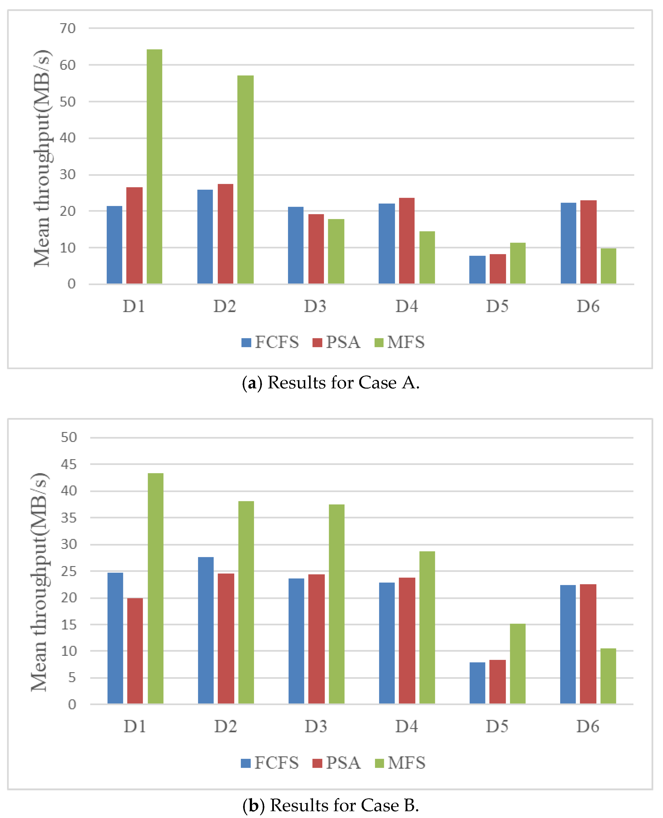
5.2.3. Mean Throughput Analysis

A task-oriented spatiotemporal data scheduling algorithm in a cloud environment should not only efficiently use network bandwidth resources but also adapt to data access preferences regarding multilevel visualization tasks. By taking the mean throughput as the index for evaluating the performance of the scheduling algorithm, comparative experiments with the FCFS, PSA and the MFS method are performed in this paper. The two algorithms are universal and have distinct characteristics. FCFS involves ordered task access, which has the advantage of fairness and disadvantage of not considering the satisfaction of scheduling. The PSA executes tasks with high priority first, thus having the advantage of considering the urgency of a task and the disadvantage of increasing the computing cost. The comparison of MFS with FCFS and PSA proves that MFS can adapt to the data access preference of multilevel visualization tasks from the two aspects of undifferentiated scheduling and priority scheduling. To ensure the reliability of the experimental results, each algorithm was assigned the same task category in the same set of scheduling tests, and the amount of data accessed by tasks was equal. Figure 13 shows the mean throughput of six types of spatiotemporal data using FCFS, PSA and the MFS method proposed in this paper; and mean throughput in Cases A and B is equivalent to the total amount of returned data divided by the task execution time.

In Figure 13a, when the demand for spatiotemporal data $D_1$ and $D_2$ requested by display tasks increases, the mean throughput of the D1 and D2 data using the MFS method is better than that of the FCFS and PSA methods, and the experimental results of FCFS and PSA are similar. In Figure 13b, the mean throughput of $D_3$, $D_4$ and $D_5$ with the maximum flow scheduling method is better than that of the FCFS and PSA methods, and the experimental results of FCFS and PSA are similar. The characteristics of the scheduling method were analyzed to determine the reasons for obtaining the experimental results. Notably, the MFS method is task-driven; when the data characteristics of a large number of task requests change, the limited-bandwidth resources can be reallocated, and more bandwidth is given to the task preference data, while other data are allocated fewer bandwidth resources at this time. Such as the mean throughput of D3, D4 and D6 data using the MFS method is smaller than that of FCFS and PSA in Case A, and mean throughput of D6 data using MFS method is smaller than that of FCFS and PSA in Case B. The FCFS and PSA methods do not have this adjustment mechanism, so there is a scramble for bandwidth resources in the data scheduling process.

In summary, the MFS method proposed in this paper can adapt to the data access preferences of multilevel visualization tasks and improve the throughput of target data. Although PSA considers the priority of tasks in scheduling, its role in improving the scheduling efficiency of target data is not as good as that of the MFS method. In addition, due to the fairness principle of FCFS for all tasks, it is unsuitable for data scheduling involving multilevel visualization tasks.

6. Conclusions

A flexible and efficient data scheduling method is the key to realizing the real-time construction and interaction of a 3D scene visualization. In this paper, the spatiotemporal data scheduling framework for multilevel visualization tasks is given. Then, the spatiotemporal data scheduling model based on the maximum flow is introduced in detail. On this basis, the task-driven maximum flow allocation method for spatiotemporal data is introduced. A virtualization container-based prototype system for data scheduling and a user-friendly web-based parameter adjustment interface are developed. The experimental results show that the MFS method addressed in this paper can support the flexible and optimized adjustment of multiple spatiotemporal data flows required by visualization tasks. The main contributions of this paper are summarized below.

First, the definitions of a multilevel visualization task and its data preference are given. Then, according to the structure of spatiotemporal data storage and scheduling in a cloud environment, the framework of spatiotemporal data scheduling is designed, which improves the theoretical basis for the optimized data scheduling.

Second, the topological network structure of spatiotemporal data scheduling is mapped to the maximum flow model, and the node and edge parameter configuration method and the detailed calculation method of multitype spatiotemporal data maximum flow are introduced. Then, two task-driven adjustment methods for the maximum flow model parameters, which improve the technical support for fine-grained spatiotemporal data optimal scheduling, are given.

Third, a prototype system based on virtualization container technology, which provides a user-friendly interface for parameter adjustment and model calculation and supports the real-time monitoring and display of multitype spatiotemporal data flow, is developed. Our system supports efficient and flexible multitype spatiotemporal data flow optimization control, providing a good paradigm for subsequent spatiotemporal data scheduling in the cloud environment.

Future research will focus on spatiotemporal data scheduling methods under multirepetition and miscellaneous architectures, such as cloud environments, edge computing and diversified clients. Meanwhile, we will further improve the adaptive adjustment ability of the spatiotemporal data scheduling service according to the diverse client task requirements.

References

1. Liu, M.; Zhu, J.; Zhu, Q.; Qi, H.; Yin, L.; Zhang, X.; Feng, B.; He, H.; Yang, W.; Chen, L. Optimization of simulation and visualization analysis of dam-failure flood disaster for diverse computing systems. Int. J. Geogr. Inf. Sci. 2017, 31, 1891–1906. [Google Scholar] [CrossRef]
2. Wu, C.; Zhu, Q.; Zhang, Y.; Du, Z.; Ye, X.; Qin, H.; Zhou, Y. A NOSQL–SQL hybrid organization and management approach for real-time geospatial data: A case study of public security video surveillance. ISPRS Int. J. Geo-Inf. 2017, 6, 21. [Google Scholar] [CrossRef] [Green Version]
3. Liu, F.; Zhang, H.; Hu, Y.; Guo, X.; Zhu, Z.; Jia, J.; Zhu, H. Cesium Based Lightweight WebBIM Technology for Smart City Visualization Management. In Proceedings of the International Conference on Inforatmion Technology in Geo-Engineering, Guimarães, Portugal, 29 September–2 October 2019; pp. 84–95. [Google Scholar]
4. Gröger, G.; Plümer, L. CityGML–Interoperable semantic 3D city models. ISPRS J. Photogramm. Remote Sens. 2012, 71, 12–33. [Google Scholar] [CrossRef]
5. Biljecki, F.; Ledoux, H.; Stoter, J. Improving the consistency of multi-LOD CityGML datasets by removing redundancy. In 3D Geoinformation Science; Springer: Cham, Switzerland, 2015; pp. 1–17. [Google Scholar]
6. Trubka, R.; Glackin, S.; Lade, O.; Pettit, C. A web-based 3D visualisation and assessment system for urban precinct scenario modelling. ISPRS J. Photogramm. Remote Sens. 2016, 117, 175–186. [Google Scholar] [CrossRef]
7. Zhang, Y.; Zhu, Q.; Liu, G.; Zheng, W.; Li, Z.; Du, Z. GeoScope: Full 3D geospatial information system case study. Geo-Spat. Inf. Sci. 2011, 14, 150. [Google Scholar] [CrossRef]
8. Zhai, W.; Chi, Z.; Fang, F.; Lv, C. Research on Spatial Data Organization for Large Scale Scene. Comput. Eng. 2003, 20. [Google Scholar]
9. Wang, W.; Lv, Z.; Li, X.; Xu, W.; Zhang, B.; Zhu, Y.; Yan, Y. Spatial query based virtual reality GIS analysis platform. Neurocomputing 2018, 274, 88–98. [Google Scholar] [CrossRef]
10. Tan, Q.; Liu, Q.; Sun, Z. Research and Application of Beijing Earthquake Disaster Prevention System Based on GIS. In Proceedings of the 2018 IEEE International Conference on Computer and Communication Engineering Technology (CCET), Beijing, China, 18–20 August 2018; pp. 275–279. [Google Scholar]
11. Li, X.; Lv, Z.; Hu, J.; Zhang, B.; Shi, L.; Feng, S. XEarth: A 3D GIS Platform for managing massive city information. In Proceedings of the 2015 IEEE International Conference on Computational Intelligence and Virtual Environments for Measurement Systems and Applications (CIVEMSA), Shenzhen, China, 12–14 June 2015; pp. 1–6. [Google Scholar]
12. Gao, P.; Liu, Z.; Xie, M.; Tian, K. The development of and prospects for private cloud GIS in China. Asian J. Geoinformatics 2015, 14. [Google Scholar]
13. Zhao, S.; Sun, X.; Chen, J.; Duan, Z.; Zhang, Y.; Zhang, Y. Relational granulation method based on quotient space theory for maximum flow problem. Inf. Sci. 2018, 507, 472–484. [Google Scholar] [CrossRef]
14. Song, W.; Jin, B.; Li, S.; Wei, X.; Li, D.; Hu, F. Building spatiotemporal cloud platform for supporting GIS application. ISPRS Ann. Photogramm. Remote Sens. Spat. Inf. Sci. 2015, 2, 55. [Google Scholar] [CrossRef] [Green Version]
15. Zhu, C.; Tan, E.C.; Chan, K. 3D Terrain visualization for Web GIS. Map Asia 2003, 13–15. [Google Scholar]
16. Su, T.; Cao, Z.; Lv, Z.; Liu, C.; Li, X. Multi-dimensional visualization of large-scale marine hydrological environmental data. Adv. Eng. Softw. 2016, 95, 7–15. [Google Scholar] [CrossRef]
17. Kang, H.-K.; Li, K.-J. A standard indoor spatial data model—OGC IndoorGML and implementation approaches. ISPRS Int. J. Geo-Inf. 2017, 6, 116. [Google Scholar] [CrossRef]
18. Ferreira, N.; Poco, J.; Vo, H.T.; Freire, J.; Silva, C.T. Visual exploration of big spatio-temporal urban data: A study of new york city taxi trips. IEEE Trans. Vis. Comput. Graph. 2013, 19, 2149–2158. [Google Scholar] [CrossRef]
19. Gaillard, J.; Peytavie, A.; Gesquiére, G. Visualisation and personalisation of multi-representations city models. Int. J. Digit. Earth 2020, 13, 627–644. [Google Scholar] [CrossRef]
20. Jaillot, V.; Servigne, S.; Gesquière, G. Delivering time-evolving 3D city models for web visualization. Int. J. Geogr. Inf. Sci. 2020, 1–23. [Google Scholar] [CrossRef]
21. Cozzi, P. Introducing 3D tiles. Cesium Blog 2015, 10. [Google Scholar]
22. Chen, Y.; Shooraj, E.; Rajabifard, A.; Sabri, S. From IFC to 3D tiles: An integrated open-source solution for visualising BIMs on cesium. ISPRS Int. J. Geo-Inf. 2018, 7, 393. [Google Scholar] [CrossRef] [Green Version]
23. Zhang, D.; Zhou, Y.; Zhang, Y. A Multi-Level Cache Framework for Remote Resource Access in Transparent Computing. IEEE Netw. 2018, 32, 140–145. [Google Scholar] [CrossRef]
24. Jin, B.; Song, W.; Zhao, K.; Wei, X.; Hu, F.; Jiang, Y. A high performance, spatiotemporal statistical analysis system based on a Spatiotemporal Cloud Platform. ISPRS Int. J. Geo-Inf. 2017, 6, 165. [Google Scholar] [CrossRef] [Green Version]
25. Pan, S.; Chong, Y.; Xu, Z.; Tan, X. An enhanced active caching strategy for data-intensive computations in distributed GIS. J. Supercomput. 2017, 73, 4324–4346. [Google Scholar] [CrossRef] [Green Version]
26. Li, R.; Wang, X.; Shi, X. A Replacement Strategy for A Distributed Caching System Based on The Spatiotemporal Access Pattern of Geospatial Data. ISPRS Ann. Photogramm. Remote Sens. Spat. Inf. Sci. 2014, 2, 133–137. [Google Scholar] [CrossRef] [Green Version]
27. Ma, T.; Hao, Y.; Shen, W.; Tian, Y.; Al-Rodhaan, M. An improved web cache replacement algorithm based on weighting and cost. IEEE Access 2018, 6, 27010–27017. [Google Scholar] [CrossRef]
28. Olanrewaju, R.F.; Baba, A.; Khan, B.U.I.; Yaacob, M.; Azman, A.W.; Mir, M.S. A study on performance evaluation of conventional cache replacement algorithms: A review. In Proceedings of the 2016 Fourth International Conference on Parallel, Distributed and Grid Computing (PDGC), Himachal Pradesh, India, 22–24 December 2016; pp. 550–556. [Google Scholar]
29. Li, R.; Feng, W.; Wu, H.; Huang, Q. A replication strategy for a distributed high-speed caching system based on spatiotemporal access patterns of geospatial data. Comput. Environ. Urban Syst. 2017, 61, 163–171. [Google Scholar] [CrossRef]
30. Ghribi, C.; Hadji, M.; Zeghlache, D. Energy efficient vm scheduling for cloud data centers: Exact allocation and migration algorithms. In Proceedings of the 2013 13th IEEE/ACM International Symposium on Cluster, Cloud, and Grid Computing, Delft, The Netherlands, 13–16 May 2013; pp. 671–678. [Google Scholar]
31. Jin, J.; Luo, J.; Song, A.; Dong, F.; Xiong, R. Bar: An efficient data locality driven task scheduling algorithm for cloud computing. In Proceedings of the 2011 11th IEEE/ACM International Symposium on Cluster, Cloud and Grid Computing, Newport Beach, CA, USA, 23–26 May 2011; pp. 295–304. [Google Scholar]
32. Bhat, M.A.; Shah, R.M.; Ahmad, B. Cloud Computing: A solution to Geographical Information Systems (GIS). Int. J. Comput. Sci. Eng. 2011, 3, 594–600. [Google Scholar]
33. Calciu, I.; Sen, S.; Balakrishnan, M.; Aguilera, M.K. How to implement any concurrent data structure for modern servers. Acm Sigops Oper. Syst. Rev. 2017, 51, 24–32. [Google Scholar] [CrossRef]
34. Kharouf, R.A.A.; Alzoubaidi, A.R.; Jweihan, M. An integrated architectural framework for geoprocessing in cloud environment. Spat. Inf. Res. 2017, 25, 89–97. [Google Scholar] [CrossRef]
35. Pignone, M.; Cogliano, R.; Moschillo, R. The development of a cloud-GIS platform for the management and sharing of geographic data during the Central Italy seismic sequence. Ann. Geophys. 2017, 59. [Google Scholar]
36. Yuan, D.; Yang, Y.; Liu, X.; Chen, J. A data placement strategy in scientific cloud workflows. Future Gener. Comput. Syst. 2010, 26, 1200–1214. [Google Scholar] [CrossRef]
37. Ziani, A.; Medouri, A. Use of cloud computing technologies for geographic information systems. In Proceedings of the International Conference on Advanced Information Technology, Services and Systems, Tangier, Morocco, 14–15 April 2017; pp. 315–323. [Google Scholar]
38. Zhan, Z.-H.; Liu, X.-F.; Gong, Y.-J.; Zhang, J.; Chung, H.S.-H.; Li, Y. Cloud computing resource scheduling and a survey of its evolutionary approaches. ACM Comput. Surv. 2015, 47, 63. [Google Scholar] [CrossRef] [Green Version]
39. Pahl, C.; Brogi, A.; Soldani, J.; Jamshidi, P. Cloud container technologies: A state-of-the-art review. IEEE Trans. Cloud Comput. 2017. [Google Scholar] [CrossRef]
40. Xavier, M.G.; Neves, M.V.; Rossi, F.D.; Ferreto, T.C.; Lange, T.; De Rose, C.A. Performance evaluation of container-based virtualization for high performance computing environments. In Proceedings of the 2013 21st Euromicro International Conference on Parallel, Distributed, and Network-Based Processing, Belfast, UK, 27 February–1 March 2013; pp. 233–240. [Google Scholar]
41. Ramkumar, K.; Gunasekaran, G. Preserving security using crisscross AES and FCFS scheduling in cloud computing. Int. J. Adv. Intell. Paradig. 2019, 12, 77–85. [Google Scholar] [CrossRef] [Green Version]
42. Arslan, S.; Topcuoglu, H.R.; Kandemir, M.T.; Tosun, O.; Computing, D. Scheduling opportunities for asymmetrically reliable caches. J. Parallel Distrib. Comput. 2019, 126, 134–151. [Google Scholar] [CrossRef]
43. Lee, Z.; Ying, W.; Wen, Z. A dynamic priority scheduling algorithm on service request scheduling in cloud computing. In Proceedings of the International Conference on Electronic & Mechanical Engineering & Information Technology, Shenyang, China, 7 September 2012; pp. 4665–4669. [Google Scholar]
44. Meng, L.; Reichenbacher, T. Map-based mobile services. In Map-based Mobile Services: Theories, Methods and Implementations; Meng, L., Reichenbacher, T., Zipf, A., Eds.; Springer: Berlin/Heidelberg, Germany, 2005; pp. 1–10. [Google Scholar] [CrossRef]
45. Peters, S.; Jahnke, M.; Murphy, C.E.; Meng, L.; Abdul-Rahman, A. Cartographic Enrichment of 3D City Models—State of the Art and Research Perspectives; Springer International Publishing: Berlin/Heidelberg, Germany, 2017. [Google Scholar]
46. Mingwei, L.; Qing, Z.; Jun, Z.; Bin, F.; Yun, L.; Junxiao, Z.; Xiao, F.; Pengcheng, Z.; Weijun, Y.; Xinwen, X. The multi-level visualization task model for multi-modal spatio-temporal data. Acta Geod. Cartogr. Sin. 2018, 47, 1098. [Google Scholar]
47. Qing, Z.; Xiao, F.U. The review of visual analysis methods of multi-modal spatio-temporal big data. Acta Geod. Cartogr. Sin. 2017, 46, 1672. [Google Scholar]
48. Goldberg, A.V.; Tarjan, R.E. Efficient maximum flow algorithms. Commun. Acm 2014, 57, 82–89. [Google Scholar] [CrossRef]
49. Everitt, T.; Hutter, M. Analytical results on the BFS vs. DFS algorithm selection problem. Part I: Tree search. In Proceedings of the Australasian Joint Conference on Artificial Intelligence, Canberra, Australia, 29 November–2 December 2020; pp. 15–165. [Google Scholar]
50. Goldfarb, D.; Grigoriadis, M.D. A computational comparison of the dinic and network simplex methods for maximum flow. Ann. Oper. Res. 1988, 13, 81–123. [Google Scholar] [CrossRef]
51. Nirmala, H.; Girijamma, H.A. Fuzzy Priority Scheduling Algorithm for Multiprocessor Systems. In Proceedings of the 2017 International Conference on Recent Advances in Electronics and Communication Technology (ICRAECT), Bangalore, India, 16–17 March 2017. [Google Scholar]
52. Zhu, Q.; Feng, B.; Li, M.; Chen, M.; Xu, Z.; Xie, X.; Zhang, Y.; Liu, M.; Huang, Z.; Feng, Y. An efficient sparse graph index method for dynamic and associated data. Acta Geodaetica et Cartographica Sinica 2020, 49, 681–691. [Google Scholar]
53. Feng, B.; Zhu, Q.; Liu, M.; Li, Y.; Zhang, J.; Fu, X.; Zhou, Y.; Li, M.; He, H.; Yang, W. An efficient graph-based spatio-temporal indexing method for task-oriented multi-modal scene data organization. ISPRS Int. J. Geo-Inf. 2018, 7, 371. [Google Scholar] [CrossRef] [Green Version]
54. Li, D.; Mei, H.; Shen, Y.; Su, S.; Zhang, W.; Wang, J.; Zu, M.; Chen, W. ECharts: A declarative framework for rapid construction of web-based visualization. Vis. Inform. 2018, 2, 136–146. [Google Scholar] [CrossRef]
Figure 1. Spatiotemporal data scheduling framework.
Ijgi 09 00518 g001
Figure 2. Definition of maximum flow model.
Ijgi 09 00518 g002
Figure 3. Maximum flow scheduling model.
Ijgi 09 00518 g003
Figure 4. Maximum flow scheduling model with all requests hit.
Ijgi 09 00518 g004
Figure 5. Flow chart of the Dinic algorithm.
Ijgi 09 00518 g005
Figure 6. Changing the cache algorithm to adjust the transmission capacity of the edge. States 1 and 2 are two cached storage states, r k m above R is the data block to be cached, r k m below R is the data block to be cached out, and the dotted line represents that the new data block entering R will change the internal cache block configuration state. On the edge, there is total transmission capacity c i j and maximum transmission capacity c i j k of each D k in this state. In the examples, 1f and 2f represent the allocated data flow for each type of data D k on the edge ( R M ,   M D k ) .
Ijgi 09 00518 g006
Figure 7. Screenshots of a typical three-level visualization task scene.
Ijgi 09 00518 g007aIjgi 09 00518 g007b
Figure 8. Maximum flow scheduling model of experimental spatiotemporal data.
Ijgi 09 00518 g008
Figure 9. Web-based spatiotemporal data maximum flow management interface.
Ijgi 09 00518 g009
Figure 10. The real-time throughput monitoring curves of D 1 and D 2 .
Ijgi 09 00518 g010
Figure 11. The real-time throughput monitoring curves of D 3 , D 4 and D 5 .
Ijgi 09 00518 g011
Figure 12. Adjustments of the maximum flow scheduling (MFS) model cause changes in the actual monitoring throughput.
Ijgi 09 00518 g012aIjgi 09 00518 g012b
Figure 13. Mean throughput of come first serve (FCFS), priority scheduling algorithm (PSA) and the MFS method.
Ijgi 09 00518 g013