POI Mining for Land Use Classification: A Case Study


Abstract
:1. Introduction
2. State of the Art
2.1. Data
2.1.1. Remote Sensing Images
2.1.2. Crowdsourced Data
Points of Interest (POIs)
Text Messages
Check-in Activities from LBSNs
2.1.3. OpenStreetMap (OSM) Datasets
2.1.4. Taxi Trajectories
2.1.5. Building Blocks
2.2. Methods
2.2.1. Object-Oriented Classification (OOC)
2.2.2. Latent Dirichlet Allocation (LDA)
2.2.3. K-Means
2.2.4. Hierarchical Semantic Cognition (HSC)
2.2.5. Random Forest (RF)
2.2.6. Support Vector Machine (SVM)
2.2.7. Deep Convolutional Neural Network (DCNN)
2.3. Comparative Analysis
3. Proposed Approach
3.1. Study Area
3.2. POI Mining
- North:
- ○
- West: 39.06471838, −9.50052661
- ○
- East: 39.06471838, −8.49097213
- South:
- ○
- West: 38.40907442, −9.50052661
- ○
- East: 38.40907442, −8.49097213
3.3. Ground Truth Data
Data Preparation
3.4. Feature Extraction
3.5. Feature Selection
3.6. Classification
4. Results and Discussion
5. Conclusions and Future Work
Supplementary Materials
Author Contributions
Funding
Conflicts of Interest
References
- Susanti, R.; Soetomo, S.; Buchori, I.; Brotosunaryo, P.M. Smart Growth, Smart City and Density: In Search of The Appropriate Indicator for Residential Density in Indonesia. Procedia-Soc. Behav. Sci. 2016, 227, 194–201. [Google Scholar] [CrossRef] [Green Version]
- Liu, X.; He, J.; Yao, Y.; Zhang, J.; Liang, H.; Wang, H.; Hong, Y. Classifying urban land use by integrating remote sensing and social media data. Int. J. Geogr. Inf. Sci. 2017, 31, 1675–1696. [Google Scholar] [CrossRef]
- Zhang, Y.; Li, Q.; Huang, H.; Wu, W.; Du, X.; Wang, H. The combined use of remote sensing and social sensing data in fine-grained urban land use mapping: A case study in Beijing, China. Remote Sens. 2017, 9, 865. [Google Scholar] [CrossRef] [Green Version]
- Zhang, X.; Du, S.; Wang, Q. Hierarchical semantic cognition for urban functional zones with VHR satellite images and POI data. ISPRS J. Photogramm. Remote Sens. 2017, 132, 170–184. [Google Scholar] [CrossRef]
- NOAA. National Ocean Service Website. What Is the Difference between Land Cover and Land Use? 2018. Available online: https://oceanservice.noaa.gov/facts/lclu.html (accessed on 13 March 2019).
- Gao, S.; Janowicz, K.; Couclelis, H. Extracting urban functional regions from points of interest and human activities on location-based social networks. Trans. GIS 2017, 21, 446–467. [Google Scholar] [CrossRef]
- Blaschke, T.; Hay, G.J.; Kelly, N.M.; Lang, S.; Hofmann, P.; Addink, E.A.; Feitosa, R.Q.; Van Der Meer, F.; Van Der Werff, H.; Van Coillie, F.; et al. Geographic Object-Based Image Analysis - Towards a new paradigm. ISPRS J. Photogramm. Remote Sens. 2014, 87, 180–191. [Google Scholar] [CrossRef] [Green Version]
- Terroso-Saenz, F.; Muñoz, A. Land use discovery based on Volunteer Geographic Information classification. Expert Syst. Appl. 2020, 140, 112892. [Google Scholar] [CrossRef]
- Xing, H.; Meng, Y. Integrating landscape metrics and socioeconomic features for urban functional region classification. Comput. Environ. Urban Syst. 2018, 72, 134–145. [Google Scholar] [CrossRef]
- Brennan, R.; Webster, T.L. Object-oriented land cover classification of lidar-derived surfaces. Can. J. Remote Sens. 2006, 32, 162–172. [Google Scholar] [CrossRef]
- Gong, B.; Im, J.; Mountrakis, G. An artificial immune network approach to multi-sensor land use/land cover classification. Remote Sens. Environ. 2011, 115, 600–614. [Google Scholar] [CrossRef]
- Qi, Z.; Yeh, A.G.O.; Li, X.; Lin, Z. A novel algorithm for land use and land cover classification using RADARSAT-2 polarimetric SAR data. Remote Sens. Environ. 2012, 118, 21–39. [Google Scholar] [CrossRef]
- Yao, Y.; Li, X.; Liu, X.; Liu, P.; Liang, Z.; Zhang, J.; Mai, K. Sensing spatial distribution of urban land use by integrating points-of-interest and Google Word2Vec model. Int. J. Geogr. Inf. Sci. 2017, 31, 825–848. [Google Scholar] [CrossRef]
- Zhang, X.; Du, S.; Wang, Q. Integrating bottom-up classification and top-down feedback for improving urban land-cover and functional-zone mapping. Remote Sens. Environ. 2018, 212, 231–248. [Google Scholar] [CrossRef]
- Huang, B.; Zhao, B.; Song, Y. Urban land-use mapping using a deep convolutional neural network with high spatial resolution multispectral remote sensing imagery. Remote Sens. Environ. 2018, 214, 73–86. [Google Scholar] [CrossRef]
- Durduran, S.S. Automatic classification of high resolution land cover using a new data weighting procedure: The combination of k-means clustering algorithm and central tendency measures (KMC-CTM). Appl. Soft Comput. J. 2015, 35, 136–150. [Google Scholar] [CrossRef]
- Deng, Z.; Zhu, X.; He, Q.; Tang, L. Land use/land cover classification using time series Landsat 8 images in a heavily urbanized area. Adv. Sp. Res. 2019, 63, 2144–2154. [Google Scholar] [CrossRef]
- Zhong, Y.; Zhu, Q.; Zhang, L. Scene classification based on the multifeature fusion probabilistic topic model for high spatial resolution remote sensing imagery. IEEE Trans. Geosci. Remote Sens. 2015, 53, 6207–6222. [Google Scholar] [CrossRef]
- Zhai, W.; Bai, X.; Shi, Y.; Han, Y.; Peng, Z.-R.; Gu, C. Beyond Word2vec: An approach for urban functional region extraction and identification by combining Place2vec and POIs. Comput. Environ. Urban Syst. 2019, 74, 1–12. [Google Scholar] [CrossRef]
- García-Palomares, J.C.; Salas-Olmedo, M.H.; Moya-Gómez, B.; Condeço-Melhorado, A.; Gutiérrez, J. City dynamics through Twitter: Relationships between land use and spatiotemporal demographics. Cities 2018, 72, 310–319. [Google Scholar] [CrossRef]
- Yuan, J.; Zheng, Y.; Xie, X. Discovering Regions of Different Functions in a City Using Human Mobility and POIs. SIGKDD Int. Conf. Knowl. Discov. Data Min. 2012. [Google Scholar] [CrossRef]
- Liu, X.; Niu, N.; Liu, X.J.; Jin, H.; Ou, J.P.; Jiao, L.M.; Liu, Y.L. Characterizing mixed-use buildings based on multi-source big data. Int. J. Geogr. Inf. Sci. 2018, 32, 738–756. [Google Scholar]
- Jendryke, M.; Balz, T.; McClure, S.C.; Liao, M. Putting people in the picture: Combining big location-based social media data and remote sensing imagery for enhanced contextual urban information in Shanghai. Comput. Environ. Urban Syst. 2017, 62, 99–112. [Google Scholar] [CrossRef] [Green Version]
- Lansley, G.; Longley, P.A. The geography of Twitter topics in London. Comput. Environ. Urban Syst. 2016, 58, 85–96. [Google Scholar] [CrossRef] [Green Version]
- Cheng, Z.; Caverlee, J.; Lee, K.; Sui, D.Z. Exploring Millions of Footprints in Location Sharing Services. Int. Conf. Weblogs Soc. Media 2011, 2010, 81–88. [Google Scholar]
- Arsanjania, J.J.; Vaz, E. An assessment of a collaborative mapping approach for exploring land use patterns for several European metropolises. Int. J. Appl. Earth Obs. Geoinf. 2015, 35, 329–337. [Google Scholar] [CrossRef]
- Yuan, N.J.; Zheng, Y.; Xie, X.; Wang, Y.; Zheng, K.; Xiong, H. Discovering urban functional zones using latent activity trajectories. IEEE Trans. Knowl. Data Eng. 2015, 27, 712–725. [Google Scholar] [CrossRef]
- Gong, L.; Liu, X.; Wu, L.; Liu, Y. Inferring trip purposes and uncovering travel patterns from taxi trajectory data. Cartogr. Geogr. Inf. Sci. 2016, 43, 103–114. [Google Scholar] [CrossRef]
- Trevino, A. Introduction to K-Means Clustering. Oracle + DataScience.com. 2016. Available online: https://www.datascience.com/blog/k-means-clustering (accessed on 20 March 2019).
- Jiang, S.; Alves, A.; Rodrigues, F.; Ferreira, J.; Pereira, F.C. Mining point-of-interest data from social networks for urban land use classification and disaggregation. Comput. Environ. Urban Syst. 2015, 53, 36–46. [Google Scholar] [CrossRef] [Green Version]
- Patel, S. Chapter 2: SVM (Support Vector Machine)—Theory. Machine Learning 101. 2017. Available online: https://medium.com/machine-learning-101/chapter-2-svm-support-vector-machine-theory-f0812effc72 (accessed on 10 June 2019).
- Sotiropoulos, D.N.; Tsihrintzis, G.A. Machine Learning Paradigms. In Machine Learning Paradigms: Artificial Immune Systems and Their Applications in Software Personalization; Springer International Publishing: Cham, Switzerland, 2017; pp. 107–129. [Google Scholar]
- Zhang, X.; Du, S. A Linear Dirichlet Mixture Model for decomposing scenes: Application to analyzing urban functional zonings. Remote Sens. Environ. 2015, 169, 37–49. [Google Scholar] [CrossRef]
- Lilleberg, J.; Zhu, Y.; Zhang, Y. Support vector machines and word2vec for text classification with semantic features. In Proceedings of the 2015 IEEE 14th International Conference on Cognitive Informatics & Cognitive Computing (ICCI*CC), Beijing, China, 6–8 July 2015; pp. 136–140. [Google Scholar]
- Zhang, L.; Zhang, L.; Du, B. Deep learning for remote sensing data: A technical tutorial on the state of the art. IEEE Geosci. Remote Sens. Mag. 2016, 4, 22–40. [Google Scholar] [CrossRef]
- Zhan, X.; Ukkusuri, S.V.; Zhu, F. Inferring Urban Land Use Using Large-Scale Social Media Check-in Data. Netw. Spat. Econ. 2014, 14, 647–667. [Google Scholar] [CrossRef]
- Frias-Martinez, V.; Frias-Martinez, E. Spectral clustering for sensing urban land use using Twitter activity. Eng. Appl. Artif. Intell. 2014, 35, 237–245. [Google Scholar] [CrossRef] [Green Version]
- Yao, Y.; Liang, H.; Li, X.; Zhang, J.; He, J. Sensing urban land-use patterns by integrating Google Tensorflow and scene-classification models. Int. Arch. Photogramm. Remote Sens. Spat. Inf. Sci.-ISPRS Arch. 2017, 42, 981–988. [Google Scholar] [CrossRef] [Green Version]
- Song, J.; Lin, T.; Li, X.; Prishchepov, A.V. Mapping Urban Functional Zones by Integrating Very High Spatial Resolution Remote Sensing Imagery and Points of Interest: A Case Study of Xiamen, China. Remote Sens. 2018, 10, 1737. [Google Scholar] [CrossRef] [Green Version]
- Zhang, C.; Sargent, I.; Pan, X.; Li, H.; Gardiner, A.; Hare, J.; Atkinson, P. An object-based convolutional neural network (OCNN) for urban land use classification. Remote Sens. Environ. 2018, 216, 57–70. [Google Scholar] [CrossRef] [Green Version]
- Flores, E.; Zortea, M.; Scharcanski, J. Dictionaries of deep features for land-use scene classification of very high spatial resolution images. Pattern Recognit. 2019, 89, 32–44. [Google Scholar] [CrossRef]
- Zhang, C.; Sargent, I.; Pan, X.; Li, H.; Gardiner, A.; Hare, J.; Atkinson, P. Joint Deep Learning for land cover and land use classification. Remote Sens. Environ. 2019, 221, 173–187. [Google Scholar] [CrossRef] [Green Version]
- Facebook. Places Search API for Web. Available online: https://developers.facebook.com/docs/places/web/search/ (accessed on 8 July 2020).
- Facebook. Place Information. Available online: https://developers.facebook.com/docs/graph-api/reference/place-information (accessed on 8 July 2020).
- Copernicus. CORINE Land Cover. Available online: https://land.copernicus.eu/pan-european/corine-land-cover (accessed on 2 March 2020).
- Copernicus. CLC 2018. Available online: https://land.copernicus.eu/pan-european/corine-land-cover/clc2018?tab=metadata (accessed on 8 July 2020).
- Kosztra, B.; Büttner, G.; Hazeu, G.; Arnold, S. Updated CLC illustrated nomenclature guidelines. 2019. [Google Scholar]
- Calegari, G.R.; Carlino, E.; Peroni, D.; Celino, I. Extracting urban land use from linked open geospatial data. ISPRS Int. J. Geo-Inf. 2015, 4, 2109–2130. [Google Scholar] [CrossRef]
- Facebook. All Categories. Available online: https://www.facebook.com/pages/category/ (accessed on 16 December 2019).
- Novaković, J.; Strbac, P.; Bulatović, D. Toward optimal feature selection using ranking methods and classification algorithms. Yugosl. J. Oper. Res. 2011, 21, 119–135. [Google Scholar] [CrossRef]
- RapidMiner. RapidMiner | Data Science & Machine Learning Platform. 2020. Available online: https://rapidminer.com/ (accessed on 18 June 2019).
- RapidMiner. Neural Net. Available online: https://docs.rapidminer.com/latest/studio/operators/modeling/predictive/neural_nets/neural_net.html (accessed on 8 July 2020).


| Ref. | Data | Method | Objective |
|---|---|---|---|
| [37] | Twitter activity | Self-organizing maps (SOM) | Land segmentation with geolocated data |
| Spectral clustering | Detect urban land uses | ||
| [36] | Location-based social networks (LBSN) user activities, points of interest (POIs) | Laplacian score (LS) | Feature selection |
| Clustering (various algorithms) | Land use inference | ||
| Naïve Bayes (NB); Support vector machine (SVM); random forest (RF) | Classify land use | ||
| [30] | Points of interest (POIs), aggregate census employment data, boundaries of towns | POI matching algorithm | Map POIs from one source to another |
| Bayesian networks; tree-based learners; instance-based learners; rule-based learners | Classify POIs | ||
| Maximum likelihood estimation (MLE) | Estimate disaggregated land use | ||
| [16] | Land cover dataset (remote images + extra attributes) | Multi-resolution segmentation | Image segmentation |
| K-means | Define data belonging to each class | ||
| Central tendency measures | Get the central tendency measure of each class | ||
| K-nearest neighbor (K-NN); extreme learning machine (ELM); Support vector machine (SVM) | Detection of urban land cover | ||
| [27] | POIs, taxi trajectories, public transit records | Dilatation | Remove unnecessary details for map segmentation |
| Subfield-based parallel thinning algorithm | Extract the skeleton of the road segments | ||
| Two-pass algorithm | Generate segmented regions | ||
| Latent Dirichlet allocation (LDA) | Discovery of region topics using mobility patterns based on mobility semantics and location semantics | ||
| Dirichlet multinomial regression (DMR) | |||
| [4] | Remote sensing images, POIs | Hierarchical semantic cognition (HSC) | Classify urban functional zones |
| Multiresolution segmentation | Segment remote sensing images | ||
| Random forest (RF) | Label categories of land use image objects | ||
| ISO- DATA algorithm | Automatically cluster spatial object patterns | ||
| [3] | OpenStreetMaps (OSM) road network, remote sensing images, POIs, LBSN user posts | Cellular automata model | Generate the urban land use parcels |
| RF | Land use classification | ||
| Object-based classification | Classify preprocessed remote sensing images | ||
| Gray-level co-occurrence matrix (GLCM) | Calculate texture attributes | ||
| [2] | OSM road network, remote sensing images, POIs, LBSN user activities | Scale invariant feature transform (SIFT) | Extract features from remote sensing images |
| K-means | Classify features | ||
| Probabilistic latent semantic analysis (pLSA) | Identify latent semantic features | ||
| LDA | |||
| SVM | Classify urban land use types | ||
| [6] | POIs, LBSN user activities | LDA | Generate summaries of thematic place topics |
| K-means | Group semantically similar regions | ||
| Delaunay triangulation spatial constraints | |||
| Ward clustering | Identify topological and hierarchical relations | ||
| [13] | POIs, traffic analysis zones (TAZ) | Greedy algorithm | Construct the TAZ-based documents |
| Word2Vec | Extract POI vectors | ||
| K-means | Group TAZs | ||
| RF | Land use classification | ||
| [38] | Remote sensing images | TF-IDF algorithm | Transform the word frequencies into semantic features |
| RF | Classify urban land use patterns | ||
| Google Inception v5 | Detect land use patterns | ||
| [9] | POIs, text messages, building-level blocks | LDA | Calculate semantic information from crowdsourced data (text messages) |
| RF | Classify functional regions | ||
| [39] | Remote sensing images, POIs, road network | Example-based feature extraction | Produce a binary built-up/non-built-up land cover map |
| Multi-resolution segmentation | Image segmentation | ||
| Object-based classification | Urban land cover classification | ||
| [15] | Remote sensing images, road blocks | Skeleton-based decomposition method | Decompose multispectral image |
| Semi-transfer deep convolutional neural network | Land use mapping | ||
| [22] | LBSN user activities, remote sensing images, taxi trajectories, POIs | Inverse distance weight (IDW) function | Construct the relationships of different data types |
| Kernel density estimation | Infer buildings’ mixed-use functions | ||
| A modified Bayesian model | Calculate the probability of purposes of passengers based on taxi data and POIs | ||
| [14] | Remote sensing images, road blocks | Multiresolution segmentation | Segment blocks |
| Hierarchical Semantic Cognition (HSC) | Bottom-up classification (land covers and functional zones) | ||
| Inverse hierarchical semantic cognition (IHSC) | Optimize classification results | ||
| [40] | Remote sensing images | Object-based convolutional neural network | Urban land use classification |
| [19] | POIs, origin–destination (OD) datasets | K-means | Group POIs and cluster neighborhood areas |
| POI frequency analysis | Annotate the function of each region | ||
| RF | Evaluate and compare the model accuracy | ||
| Place2vec | Extract and classify urban functional regions | ||
| [41] | Remote sensing images | ResNet-50 DCNN | Extract the deep features from images |
| [17] | Remote sensing images | Space–time fusion algorithm (ESTARFM) | Fuse original data pairs at two periods |
| Multiresolution segmentation | Segment the images | ||
| SVM | Extract land use and land cover types | ||
| [42] | Remote sensing images | Joint deep learning (JDL) | Land use and land cover classification |
| [8] | Flickr photos, POIs | Hierarchical clustering LDA RF Multi-label classification | Cluster photos to identify most dynamic regions Extract topics from photo descriptions Land use classification on POI taxonomy (ground truth) using LDA topics as features |
| Ours | POIs | Artificial neural network (ANN) (please see Section 3.6) | Using CORINE (CLC) dataset as ground truth (Section 3.3), extract features from POI taxonomy (Section 3.4) to learn a land use classifier |
| Class | Subclass |
|---|---|
| Class 1.1. Urban fabric | 111. Continuous urban fabric |
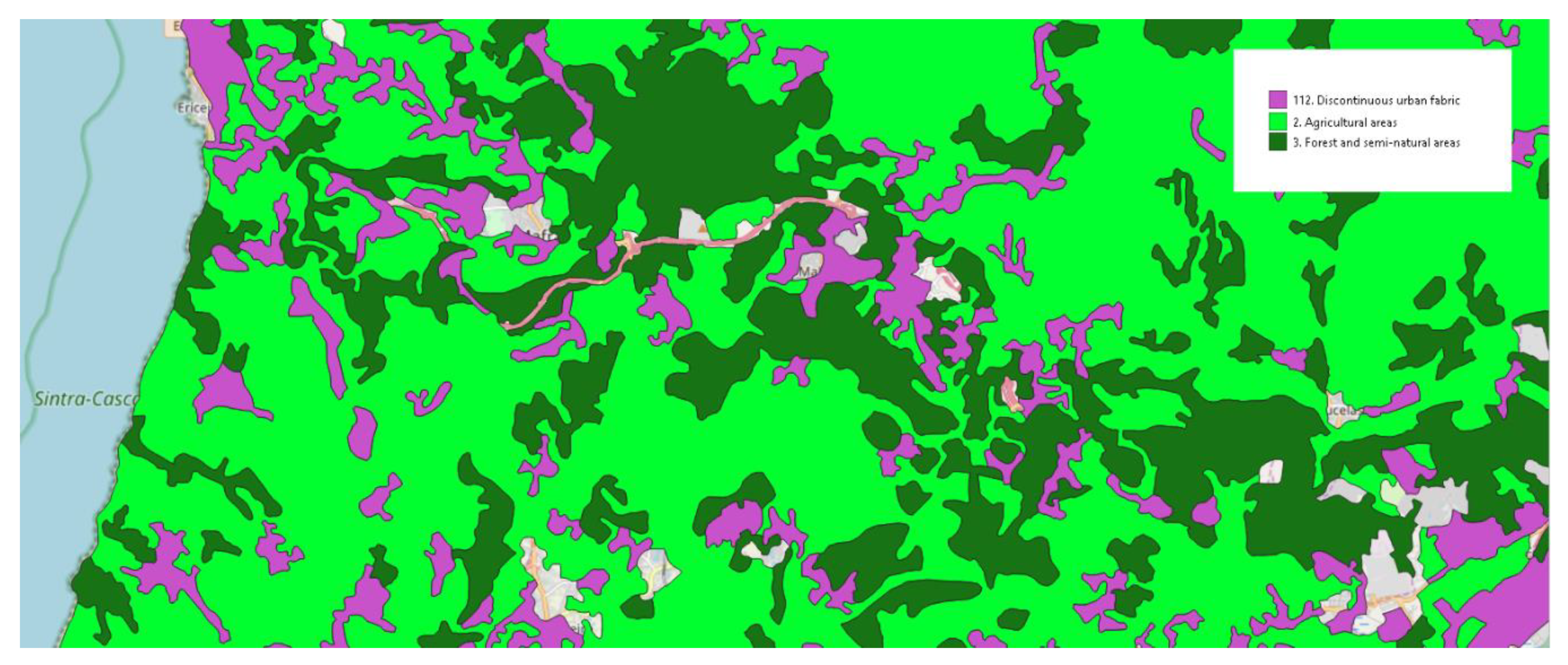
| 112. Discontinuous urban fabric | |
| Class 1.2. Industrial, commercial and transport units | 121. Industrial or commercial units and public facilities |
| 122. Road and rail networks and associated land | |
| 123. Port areas | |
| 124. Airports | |
| Class 1.3. Mine, dump and construction sites | 131. Mineral extraction sites |
| 132. Dump sites | |
| 133. Construction sites | |
| Class 1.4. Artificial non-agricultural vegetated areas | 141. Green urban areas |
| 142. Sport and leisure facilities | |
| 2. Agricultural areas | 2. Agricultural areas |
| 3. Forest and semi-natural areas | 3. Forest and semi-natural areas |
| 4. Wetlands | 4. Wetlands |
| 5. Water bodies | 5. Water bodies |
| Feature Set | Description |
|---|---|
| Group 1 | Distance from each cell centroid to the closest POI of each category |
| Group 2 | Distance from each cell centroid to the most distant POI of each category |
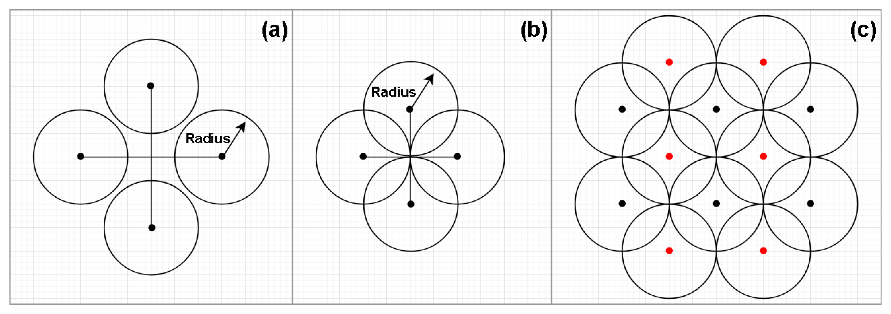
| Group 3 | Amount of POIs belonging to each category inside a radius from each centroid |
| Group 4 | Proportion of POIs belonging to each category inside a radius from each centroid |
| Classifier | Parameter | Value |
|---|---|---|
| Artificial neural network—ANN | Hidden layers | (Number of attributes + number of classes)/2 + 1 |
| Training cycles | 200 | |
| Learning rate | 0.01 | |
| Momentum | 0.9 | |
| Shuffle | True | |
| Normalize | True | |
| Error epsilon | 0.0001 |
| Measure | Value | Class | Prec. | Recall | F-Score |
|---|---|---|---|---|---|
| Accuracy | 77.41 | 2. Agricultural areas | 83.32 | 76.30 | 79.66 |
| Weighted F-score | 77.39 | 111. Continuous urban fabric | 78.74 | 88.24 | 83.22 |
| Kappa | 0.70 | 112. Discontinuous urban fabric | 69.94 | 71.65 | 70.78 |
| Weighted recall | 77.89 | 121. Industrial or commercial units and public facilities | 79.17 | 75.37 | 77.22 |
| Weighted precision | 78.22 |
| Measure | Value | Class | Prec. | Recall | F-Score |
|---|---|---|---|---|---|
| Accuracy | 78.53 | 3. Forest and semi-natural areas | 87.27 | 82.45 | 84.79 |
| Weighted F-score | 72.14 | 111. Continuous urban fabric | 76.25 | 87.91 | 81.68 |
| Kappa | 0.71 | 112. Discontinuous urban fabric | 74.31 | 70.28 | 72.24 |
| Weighted recall | 78.74 | 121. Industrial or commercial units and public facilities | 75.09 | 74.35 | 74.72 |
| Weighted precision | 78.65 |
| Measure | Value | Class | Prec. | Recall | F-Score |
|---|---|---|---|---|---|
| Accuracy | 78.01 | 2. Agricultural areas | 76.93 | 66.12 | 71.12 |
| Weighted F-score | 77.86 | 3. Forest and semi-natural areas | 72.90 | 79.07 | 75.86 |
| Kappa | 0.70 | 111. Continuous urban fabric | 87.54 | 90.04 | 88.77 |
| Weighted recall | 78.94 | 121. Industrial or commercial units and public facilities | 76.60 | 80.50 | 78.50 |
| Weighted precision | 78.57 |
| Measure | Value | Class | Prec. | Recall | F-Score |
|---|---|---|---|---|---|
| Accuracy | 73.34 | 3. Forest and semi-natural areas | 72.84 | 75.58 | 74.18 |
| Weighted F-score | 71.74 | 2. Agricultural areas | 70.04 | 64.65 | 67.24 |
| Kappa | 0.64 | 111. Continuous urban fabric | 82.29 | 89.16 | 85.59 |
| Weighted recall | 74.28 | 112. Discontinuous urban fabric | 69.42 | 67.75 | 68.57 |
| Weighted precision | 73.92 |
| Measure | Value | Class | Prec. | Recall | F-Score |
|---|---|---|---|---|---|
| Accuracy | 90.21 | 2. Agricultural areas | 93.68 | 91.55 | 92.60 |
| Weighted F-score | 90.20 | 111. Continuous urban fabric | 87.75 | 93.53 | 91.60 |
| Kappa | 0.85 | 121. Industrial or commercial units and public facilities | 85.59 | 84.40 | 84.99 |
| Weighted recall | 89.83 | ||||
| Weighted precision | 89.84 |
| Measure | Value | Class | Prec. | Recall | F-Score |
|---|---|---|---|---|---|
| Accuracy | 82.31 | 111. Continuous urban fabric & 112. Discontinuous urban fabric | 81.22 | 81.17 | 81.19 |
| Weighted F-score | 82.34 | ||||
| Kappa | 0.73 | 2. Agricultural areas | 86.65 | 83.08 | 84.83 |
| Weighted recall | 82.37 | 121. Industrial or commercial units and public facilities | 77.98 | 82.86 | 80.35 |
| Weighted precision | 82.16 |
| Measure | Value | Class | Prec. | Recall | F-Score |
|---|---|---|---|---|---|
| Accuracy | 81.88 | 2. Agricultural areas & 3. Forest and semi-natural areas | 84.08 | 84.9 | 84.49 |
| Weighted F-score | 81.89 | ||||
| Kappa | 0.72 | 111. Continuous urban fabric & 112. Discontinuous urban fabric | 79.97 | 81.15 | 80.56 |
| Weighted recall | 81.83 | ||||
| Weighted precision | 81.75 | 121. Industrial or commercial units and public facilities | 81.44 | 78.58 | 79.98 |
| 2. Agricultural Areas | 111. Continuous Urban Fabric | 112. Discontinuous Urban Fabric | 121. Industrial or Commercial Units and Public Facilities | |||||
|---|---|---|---|---|---|---|---|---|
| 2. Agricultural areas | 3052 | 76.74% | 15 | 0.49% | 466 | 11.65% | 130 | 4.87% |
| 111. Continuous urban fabric | 83 | 2.09% | 2685 | 88.24% | 409 | 10.23% | 233 | 8.74% |
| 112. Discontinuous urban fabric | 661 | 16.62% | 257 | 8.45% | 2866 | 71.65% | 294 | 11.02% |
| 121. Industrial or commercial units and public facilities | 181 | 4.55% | 86 | 2.83% | 259 | 6.48% | 2010 | 75.37% |
© 2020 by the authors. Licensee MDPI, Basel, Switzerland. This article is an open access article distributed under the terms and conditions of the Creative Commons Attribution (CC BY) license (http://creativecommons.org/licenses/by/4.0/).
Share and Cite
Andrade, R.; Alves, A.; Bento, C. POI Mining for Land Use Classification: A Case Study. ISPRS Int. J. Geo-Inf. 2020, 9, 493. https://doi.org/10.3390/ijgi9090493
Andrade R, Alves A, Bento C. POI Mining for Land Use Classification: A Case Study. ISPRS International Journal of Geo-Information. 2020; 9(9):493. https://doi.org/10.3390/ijgi9090493
Chicago/Turabian StyleAndrade, Renato, Ana Alves, and Carlos Bento. 2020. "POI Mining for Land Use Classification: A Case Study" ISPRS International Journal of Geo-Information 9, no. 9: 493. https://doi.org/10.3390/ijgi9090493
APA StyleAndrade, R., Alves, A., & Bento, C. (2020). POI Mining for Land Use Classification: A Case Study. ISPRS International Journal of Geo-Information, 9(9), 493. https://doi.org/10.3390/ijgi9090493