Helmert Transformation Problem. From Euler Angles Method to Quaternion Algebra

Abstract

The three-dimensional coordinate’s transformation from one system to another, and more specifically, the Helmert transformation problem, is one of the most well-known transformations in the field of engineering. In this paper, its solution, in reverse problem, was investigated for specific data using three different methods. It is presented by solving it with the method of Euler angles as well as with the use of quaternion and dual-quaternion algebra, after first giving some basic mathematical theory. After research, not only were three artificial sets of data used, which were structured in a specific way and forced into specific transformations to be solved, but also a real geodesy problem was tested, in order to identify the sensitivity and problems of each method. Statistical analysis of the results was performed by each method, while it was found that there were significant deviations in rotations and translations in the method of Euler angles and dual quaternions, respectively.

1. Introduction

Coordinate (system) transformation is a well-known mathematical process that is often used in geodesy, photogrammetry, geographical information science (GIS), computer vision, and in many other branches of engineering. Coordinates from the World Geodetic System 1984 (WGS84) to local systems from local systems to specific object systems or transformations of Lidar point clouds are only a few applications of that process [1]. This can be used either as a direct problem or as a reverse. In the first case, the points are transferred from one system to another, knowing the relationship between the two systems, while in the second case, points are given to both systems and the relationship of one system to the other is requested.

In most geodetic applications, both transformations are done in two dimensions as the altimeter reference remains unchanged, but things become more complicated when three-dimensional point transformation is required. Rotations through all three axes, 3D vector displacement as well as single scale change, are calculated in order to transfer points from one system to another. These seven transformation parameters are known as the 7-parameter transformation or Helmert transformation problem, which is a well-known transformation, not only in engineering, but also in most sciences [1,2].

A bibliographic survey found that calculating the rotation matrix often causes significant problems. Nowadays, the most classic way of determining it is by using Euler angles, where it is defined by using the sines and cosines of the angles for each axis rotation [3]. Thus, complementary angles have the same values of trigonometric numbers, resulting in different angles from the same rotation matrix.

In order to deal with the rotation of points on the plane, in the mathematical community, simple pairs are used, where the points are given in the form of complex numbers, following all their properties. However, the problem becomes more complicated when these points are depicted in space, because simple pairs are not enough. Therefore, a solution was given by Hamilton [4], who created a new algebraic structure, the quaternions, which consist of one real and three imaginary parts i, j, and k [3,5].

The difference between the quaternions and other similar methods are interpreted geometrically. Thus, with their use, the final rotation matrix is unambiguous and consists of the coefficients of a quaternion in the form of $q=q_0+q_{1}i+q_{2}j+q_{3}k$. This quaternion is defined as the external product of individual quaternions, depending on the order in which the axes rotate, while taking into account the clockwise angle per axis [3,5].

Taking everything into account, there are two different calculating methods of rotation matrix. In this paper, after explaining how these methods compare with the Helmert transformation problem, an investigation took place to show which method was better and why.

Three different datasets were created and specific transformations took place to choose the best transformation method at any case. The transformation parameters were chosen very carefully, and axes rotation came up after special research. Moreover, an example of a geodetic problem is presented to test each methodology using real data.

After solving the reverse transformation problem, using least square method, a statistical analysis was performed, and important conclusions emerged.

2. Mathematical Context and Helmert Transformation Calculated Methods

Three-dimensional space geometry has preoccupied scientists for many years. The main problem arose when calculating the rotation matrix in 3D space. This matrix is a 3 × 3 table, which shows the rotation around a specific axis at a certain angle. This matrix is called R and is a rectangular table with a determinant equal to 1 (detR = 1 and R⁻¹ = R^T). In order to calculate this matrix, two different methods were used [6].

In the first case, the rotations for the axes x, y, z and Euler angles α, β, γ, respectively, can be calculated using $R_x(a)$, $R_y(\beta )$, $R_z(\gamma )$ [3], given by the following relations:

$${\mathrm{R}}_x(a)=\left[\begin{array}{ccc}1& 0& 0\\ 0& cos\alpha & -sin\mathsf{\alpha }\\ 0& sin\alpha & cos\alpha \end{array}\right],{\mathrm{R}}_y(\beta )=\left[\begin{array}{ccc}cos\beta & 0& sin\beta \\ 0& 1& 0\\ -sin\beta & 0& cos\beta \end{array}\right],{\mathrm{R}}_z(\gamma )=\left[\begin{array}{ccc}cos\gamma & -sin\gamma & 0\\ sin\gamma & cos\gamma & 0\\ 0& 0& 1\end{array}\right]$$

(1)

If there is more than one rotation, the Euler angle sequence is used. Each of these rotations are counter-clockwise and the coordinate system is right-handed. In that way, the order of rotations is important because there are 27 different combinations. Each rotation sequence gives different results and different rotation sequences can be used in different applications. One of the best known combinations is the “xyz rotation”, which first rotates around the x-axis, then around the y, and finally about the z, while the final rotation matrix is given by the relation ${\mathrm{R}}_{\mathrm{xyz}}=R_z(\gamma )·R_y(\beta )·R_x(a)$ [3,7]. In addition, this method causes limitations in representing the rotation of an object because, in every Euler angle sequence, there is at least one point that loses a degree of freedom. This loss is known as gimbal lock, a phenomenon where one of the rotation axis realigns with the other axis [3].

In the second case, the rotation matrix is calculated using quaternion algebra. Given Hamilton’s theory, the quaternions were defined as $q=q_0+q_{1}i+q_{2}j+q_{3}k$, where $q_0,q_1,q_2,\mathrm{and}{q}_3$ are real numbers and $i,j,k$ are imaginary units considering the conditions of $i^2=j^2=k^2=i·j·k=-1$. These numbers can be represented as a four vector element in $R^4$, of the form $q=(q_0,q_1,q_2,q_3)=(q_0,\mathit{q})$ where $q_0$ is its scalar part, $\mathit{q}=(q_1,q_2,q_3)$ its vector part, and i, j, and k are the orthonormal basis in $R^3$ [7].

In addition, based on a well-known theorem [4,8]:

Theorem: 

A unit quaternion q, written of the form $q=q_0+\mathit{q}=cos\theta +\widehat{\mathit{u}}sin\theta$, and for any vector $\mathit{v}\in R^3$, the Quaternion Rotation Operator $L_q(\mathit{v})$ is defined, where:

$$L_q(\mathit{v})=q\mathit{v}{q}^{*}=(q_0^2-{\left|\mathit{q}\right|}^2)\mathit{v}+2(\mathit{q}·\mathit{v})\mathit{q}+2q_0(\mathit{q}\times \mathit{v})$$

(2)

Thus, for the rotation of a vector $t\in R^3$ around a specific axis and based on the rotation operator, the vector $t^{\prime }$ is obtained as $t^{\prime }=Q_u·t·Q_u^{*}$ where $u$ is the axis around which the vector rotates [3,7]. In order to generalize this relationship, Hamilton’s rules for relations between i, j, and k are used and it follows that the vector $t^{\prime }$ can also be determined by the relation $t^{\prime }={\mathrm{R}}^Q·t$ where ${\mathrm{R}}^Q$ is the general quaternion rotation matrix given by the relation:

$$R^Q=\left[\begin{array}{ccc}{q}_0^2+q_1^2-q_2^2-q_3^2& 2·q_1·q_2-2·q_0·q_3& 2·q_1·q_3+2·q_0·q_2\\ 2·q_0·q_3+2·q_1·q_2& q_0^2-q_1^2+q_2^2-q_3^2& -2·q_0·q_1+2·q_2·q_3\\ -2·q_0·q_2+2·q_1·q_3& 2·q_0·q_1+2·q_2·q_3& q_0^2-q_1^2-q_2^2+q_3^2\end{array}\right]$$

(3)

However, the above relationships describe the rotation around a single axis, so it is advisable to study what happens if more than one turn occurs. As with the Euler angle method, it matters what order the rotations are performed as there are many different combinations. So, $Q_u$ is replaced by $Q_{abc}$, where abc is the order of the axes where rotation will take place. If there is a rotation about the xyz, then $Q_{xyz}=Q_z\times Q_y\times Q_x$ where $Q_{xyz}=q_o^{xyz}+q_1^{xyz}·i+q_2^{xyz}·j+q_3^{xyz}·k$.

2.1. Helmert Transformation Problem

This transformation is one of the most well-known in the world, both in the field of geodesy and photogrammetry [1,9]. It is about converting the coordinates of one set of points from one system to another when they do not have the same origin, scale, and orientation. Thus, this problem has seven transformation parameters: three transitions, three turns on axes x, y, and z, respectively, and one scale factor.

More specifically, for two systems (P) and (P′) and for each point ${\mathrm{p}}_{\mathrm{i}}={({\mathrm{x}}_{\mathrm{i}},{\mathrm{y}}_{\mathrm{i}},{\mathrm{z}}_{\mathrm{i}})}^{\mathrm{T}}$ and ${{\mathrm{p}}_{\mathrm{i}}}^{\prime }={({\mathrm{x}}_{\mathrm{i}}^{\prime },{\mathrm{y}}_{\mathrm{i}}^{\prime },{\mathrm{z}}_{\mathrm{i}}^{\prime })}^{\mathrm{T}}$, respectively, the relation holds [2]:

$${{\mathrm{p}}_{\mathrm{i}}}^{\prime }=\mathrm{t}+\mathsf{\lambda }·\mathrm{R}(\mathrm{f})·{\mathrm{p}}_{\mathrm{i}},\mathrm{i}=1,\dots ,\mathrm{m}$$

(4)

where $\mathrm{t}={\left[{\mathrm{t}}_{\mathrm{x}},{\mathrm{t}}_{\mathrm{y}},{\mathrm{t}}_{\mathrm{z}}\right]}^{\mathrm{T}}$ is the translation vector; λ is the scale factor; and $\mathrm{R}(\mathrm{f})$ is the rotation matrix through axis xyz.

If the transformation parameters are given, then it is very easy to convert points from one system to another. However, in this paper, the problem is the exact opposite. With the coordinates of some points in both systems known, the calculation of the seven parameters of the transformation is sought. The solution will be calculated using three different methods, as explained below.

2.1.1. Euler Angle Method

In this method, the rotation matrix is calculated using the Euler angle sequence. For easier calculation of the matrix, Awange and Grafarend [10] introduced the symmetrical matrix ${\mathrm{C}}^{\prime }$ where it has the property $\mathrm{R}={(\mathrm{I}-{\mathrm{C}}^{\prime })}^{-1}·(\mathrm{I}+{\mathrm{C}}^{\prime })$ with I as the unit matrix 3 × 3 and ${\mathrm{C}}^{\prime }$ (with parameters $a,b,c\in R$) is given by the relation [11]:

$${\mathrm{C}}^{\prime }=\left[\begin{array}{ccc}0& -c& b\\ c& 0& -a\\ -b& a& 0\end{array}\right]$$

(5)

In this way, the rotation matrix has three unknown parameters that are not the unknown angles but three real numbers $a,b,c$. As a result, the unknown parameters are still seven ($a,b,c$ for rotation, ${\mathrm{t}}_{\mathrm{x}},{\mathrm{t}}_{\mathrm{y}},{\mathrm{t}}_{\mathrm{z}}$ for translation, and λ for scale) and the final angles are calculated through the rotation matrix and the following equations:

$$\alpha ={\mathrm{f}}_{\mathrm{x}}=\arctan \frac{{\mathrm{R}}_{(2,3)}}{{\mathrm{R}}_{(3,3)}},\beta ={\mathrm{f}}_{\mathrm{y}}=-\arcsin {\mathrm{R}}_{(1,3)},\gamma ={\mathrm{f}}_{\mathrm{z}}=\arctan \frac{{\mathrm{R}}_{(1,2)}}{{\mathrm{R}}_{(1,1)}}$$

(6)

2.1.2. Quaternion Method

In the second method, in order to calculate the rotation matrix, quaternions are used. Using the quaternion rotation operator and the main properties of quaternions, the matrix R is calculated by the equation [11]:

$$\mathrm{R}=({\mathrm{q}}_0^2-q^{\mathrm{T}}.\mathrm{q})·{\mathrm{I}}_3+2·(\mathrm{q}·{\mathrm{q}}^{\mathrm{T}}+q_0·\mathrm{C}(q))$$

(7)

where I₃ is the unit matrix 3 × 3 and the symmetrical matrix of Equation (5), where $a=q_1,b=q_2$, $c=q_3$.

In this case, the unknown parameters are eight: the quaternion q = ($q_0,q_1,q_2,q_3$) for the rotation matrix, ${\mathrm{t}}_{\mathrm{x}},{\mathrm{t}}_{\mathrm{y}},{\mathrm{t}}_{\mathrm{z}}$ for translation and λ for scale factor. In order to calculate the final three rotation angles, the least square method is also used to estimate the values and their error.

2.1.3. Dual-Quaternion Method

The final method uses dual quaternions to calculate the transformation problem. In 1882, Clifford [12] incorporated the theory of dual numbers with quaternion algebra, creating the dual-quaternions, in order to describe both the rotation and the translation of an object with a single mathematical relation [13]. In this way, dual-quaternions are double numbers with their elements being quaternions. More specifically, they are defined as [14,15]:

$$\overline{\mathit{q}}=\mathit{r}+\mathit{d}·\epsilon \mathrm{with}\mathit{r}\mathrm{and}\mathit{d}\mathrm{being}\mathrm{quaternions}\mathrm{and}{\epsilon }^2=0\mathrm{with}\epsilon \ne 0$$

(8)

In order to determine a new position of a point, through the dual quaternions, the translation and rotation properties for the unit dual quaternion were defined as $q_r=\mathit{r}$ and $\mathit{d}=\mathit{t}·\mathit{r}$, with r the unit quaternion that represents the rotation and $\mathit{t}=(0,{\mathrm{t}}_{\mathrm{x}},{\mathrm{t}}_{\mathrm{y}},{\mathrm{t}}_{\mathrm{z}})$ the quaternion that represents the translation [1,16].

Utilizing the dual quaternion theory, the R matrix can be determined from the relation:

$$\mathrm{R}=(r_0^2-{\mathit{r}}^T·\mathit{r})·\mathrm{I}+2·(\mathit{r}·{\mathit{r}}^T+r_0·\mathrm{C}(\mathit{r}))$$

(9)

For greater convenience, $\mathrm{Q}(\mathbf{r})$ and $\mathrm{W}(\mathbf{r})$ are also defined using unit matrix I and the symmetrical matrix $\mathrm{C}(\mathit{r})$, as above:

$$\mathrm{Q}(\mathit{r})=\left[\begin{array}{cc}{r}_0·\mathrm{I}+\mathrm{C}(\mathit{r})& \mathit{r}\\ -{\mathit{r}}^{\mathrm{T}}& r_0\end{array}\right],\mathrm{W}(\mathit{r})=\left[\begin{array}{cc}{r}_0·\mathrm{I}-\mathrm{C}(\mathit{r})& \mathit{r}\\ -{\mathit{r}}^{\mathbf{T}}& r_0\end{array}\right]$$

(10)

Following the main properties of $\mathit{r},\mathit{t},\mathrm{and}\mathit{d}$, as shown below [15]:

$$\mathit{t}=\mathit{d}·{\mathit{r}}^{-1}=\mathit{d}·\frac{{\mathit{r}}^{*}}{\parallel \mathit{r}\parallel }=\mathit{d}·{\mathit{r}}^{*}=\mathrm{W}({\mathit{r}}^{*})·\mathit{d}=\mathrm{W}{(\mathit{r})}^{\mathit{T}}·\mathit{d}$$

(11)

the final transformation relation arises, where the required quaternions r and d are present.

$${\mathrm{p}}_{\mathrm{i}}^{\prime }=2·W·{(\mathit{r})}^T·\mathit{d}+\mathsf{\lambda }·\mathrm{W}{(\mathit{r})}^T·\mathrm{Q}(\mathit{r})·{\mathrm{p}}_{\mathrm{i}},\mathrm{i}=1,\dots ,\mathrm{m}$$

(12)

In this way, the unknown parameters are nine: four for each quaternion that represents the rotation and translation and one for scale factor. As above, the least square method is used to calculate both the rotation angles and the translation parameters as well as their error.

2.2. Least Square Calculating Method

As above-mentioned, in order to calculate the unknown parameters, the least square method was used. This method is known as the combined least squares technique and was chosen because the coordinates have uncertainty at both systems [17,18]. The main equation of the method is:

$$A·\widehat{x}+B·(l+u)=k$$

(13)

where $A$ is the matrix of coefficients of the parameters of interest; $B$ is the matrix of coefficients of the measured data; $\hat{x}$ is the vector of the best parameter values; $l$ is the vector of measurements; $u$ is the vector of the rest of the measurements; and $k$ is the vector of fixed terms.

In all three methods, the final transformation relations are non-linear. Therefore, because of the linearization, matrices A and B contain partial derivatives. In order to estimate the starting values, the minimum equations are solved depending on the number of unknown parameters in each method. After this process, the least square method is calculated and both the final unknown parameters and their errors are calculated [18].

3. Case Study

After explaining the Helmert transformation problem and its solution methods, it is important to check out which method is the best for the reverse problem. Thus, a case study took place.

First of all, three different datasets were created. These sets transformed using specific transformation parameters to have, as a result, three-dimensional coordinates in both systems. Taking into consideration the points, and using the least square method, transformation parameters were calculated as a reverse problem, in order to find out the main deviations from the real values. Both the deviations and their errors were statistically tested to identify the sensitivity and problems of each method [18].

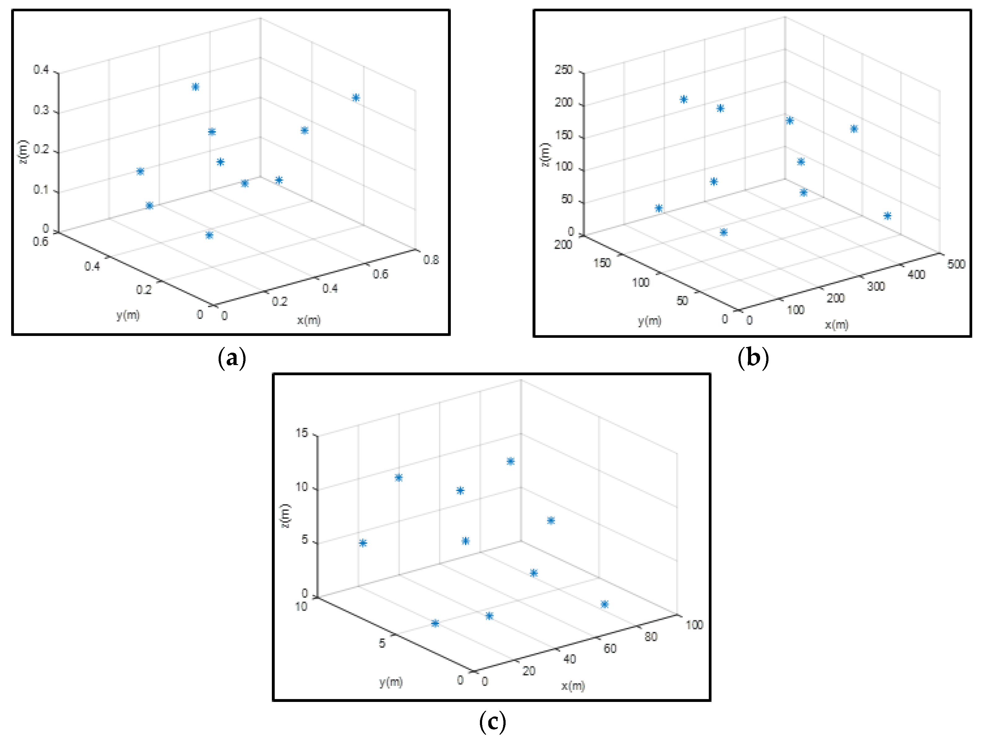
3.1. Datasets

As above-mentioned, three different datasets with ten points each chosen randomly were created. One set concerned the microcosm with the distances of the points being at most 50–70 cm apart with an accuracy of ±0.05 mm; another referred to the macrocosm with distances of 200–500 m and an accuracy of ±1 cm; and finally, there is an intermediate set with distances of 10–100 m and accuracy of ±1 mm. In Figure 1a–c, the datasets are shown in three-dimensional space.

3.2. Transformation Parameters

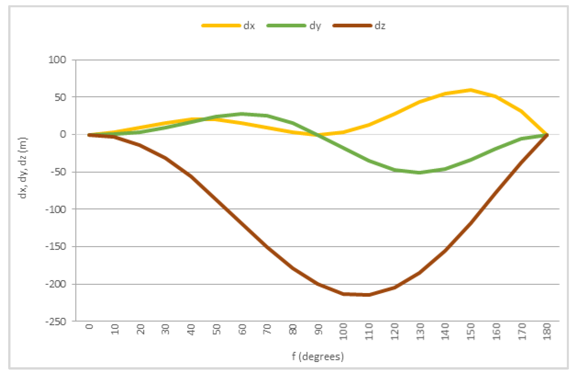
Each dataset was subjected to specific transformations. For the translation parameters, the chosen values were 0.50 m, 10 m, and 100 m at the same time on all three axes, but also separately for each. These values were also chosen randomly to test the different order of magnitudes. The scale factor was selected either by enlarging the system or by reducing it. Thus, for the specific scenarios, λ = 0.5, λ = 1, and λ = 1.5 were selected. Finally, in order to select the rotation angles, a special investigation took place.

For an initial point P (100,100,100) and transformation only for rotation (for angles 0°–180° at each axe in the order xyz), the difference of coordinates can be calculated, as shown in Figure 2. It was observed that for angles 0°–20°, the changes were very small. Respectively, for angles 80°–120°, the largest deviation was mainly in the z axis, and for angles 160°–180°, the lines of the above diagram showed a strong slope, compared to the rest of the diagram. Thus, these areas are considered “marginal and suspicious” and require further notice.

According to the above-mentioned, the rotation angles at each transformation were chosen between the problematic areas. The rotation was in the order xyz, while it was either equal to all three axes or not.

Therefore, the transformations that took place are shown in the following table. Each dataset had nine different scenarios, solved by three different methods, as shown in

Table 1. Scenarios for each dataset, which were tested for each calculation method.

Senarios ID	Translation (m)			Rotation (Degrees)			Scale Factor
	tx	ty	ty	fx(α)	fy(β)	fz(γ)	λ
1	0.50	0.50	0.50	5	5	5	0.50
2	0.50	0.50	0.50	5	5	5	1.50
3	10	10	10	100	100	100	0.50
4	10	10	10	100	100	100	1.50
5	100	100	100	170	170	170	0.50
6	100	100	100	170	170	170	1.50
7	0.50	100	10	5	100	170	0.50
8	100	0.50	100	100	5	100	1
9	10	100	0.50	170	100	5	1.50

. In this way, 27 scenarios were tested for each Helmert transformation calculating method, and the results were statistically checked. The first dataset had an ID for 1–9, the second for 10–18, and the third for 19–27. It is important to note that the uncertainty was the same for all coordinates at both systems because the determination of coordinates was considered to be done by the method of polar coordinates.

4. Results

After calculating the 27 different transformations for each method, a statistical analysis took place. Diagrams were created and deviations of the calculated quantities from the real values were calculated while a 95% confidence level check was performed. The results were tested to check the problems of each method considering the data format.

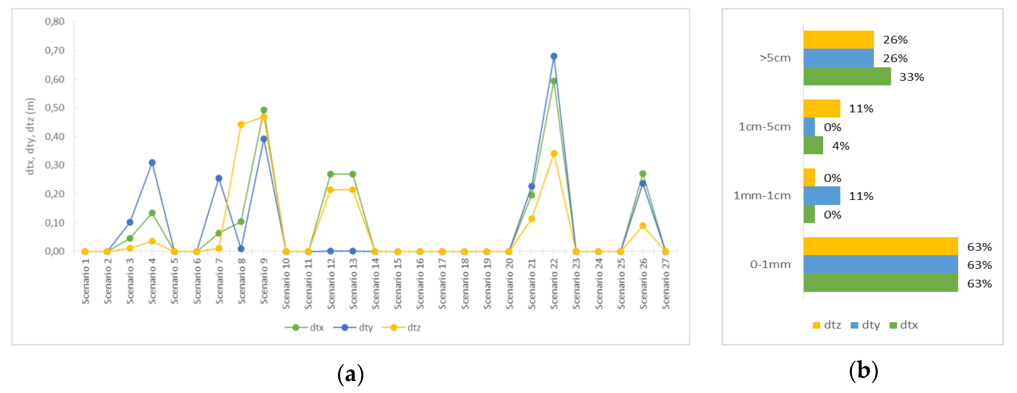
First of all, in the Euler angle method, the percentage of correct solution was only 22%, while that of the incorrect one was 78%. In all scenarios, the scale had acceptable deviations of 100%, while the values were of the order ${10}^{-5}$. For the translation, as shown in Figure 3, the deviations ranged from a few tenths of a millimeter to a few centimeters. The largest deviation reached 67 cm for scenario 22, while 63% of the scenarios had deviations less than 1 mm. It is worth noting that for the most part, the second dataset showed very small deviations, unlike the first, which showed strong fluctuations, especially in scenarios with different values per axis (Scenarios 7–9), or in those where the translation was of the order of 10 m (Scenarios 3–4). Regarding the uncertainty of the calculated values, this was of the order of ${10}^{-6}$.

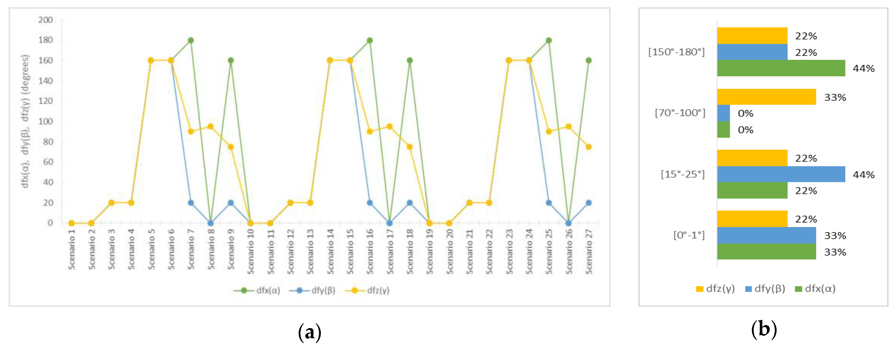
Considering the rotation angles, as shown in Figure 4, a periodicity in deviations was presented as scenarios with the same transformation parameters bring about the same deviations regardless of the form of the data. Observing the values of the calculated angles in relation to the real ones, it was found that despite their differences, the same rotation matrix emerged. This occurred for symmetrical angles in the trigonometric circle as the combination of the same trigonometric numbers with the opposite sign brings the same result.

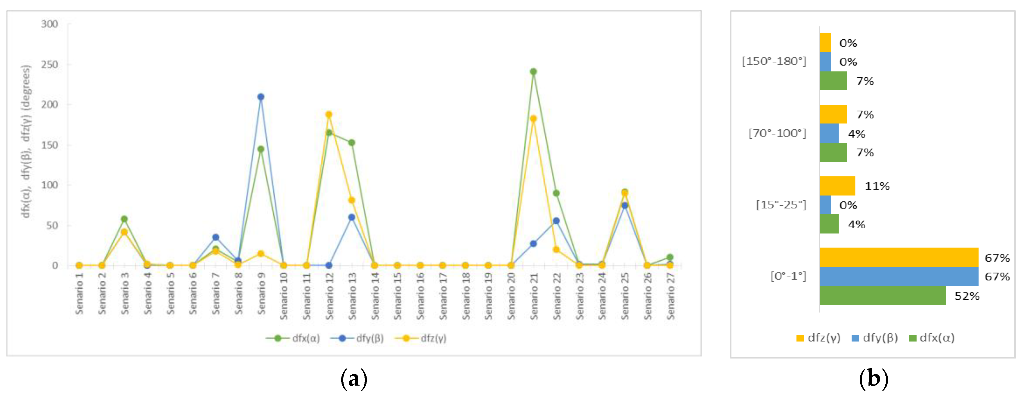
Second, in the quaternion method, the percentage of correct solution was improved in 63%. According to Figure 5, it was found that there were four scenarios that showed deviations of the order of a few meters. The largest deviation in translation reached 145 m for scenario 13, while 63–70% of the scenarios had deviations less than 1 mm. An investigation revealed that scenarios 12 and 13 and 21 and 22, which had the same characteristics and showed extreme values, were solved incorrectly during the process of finding the initial values, resulting in their huge deviation from the actual values. The same problem occurred for each transformation parameter, both in rotation and scale factor. As for the uncertainty of the calculated translation, this was of the order of ${10}^{-5}$ or even a few centimeters, with the exception of problematic scenarios, which could reach 20 m.

Regarding the scale, it was observed that in the majority of scenarios, the deviations were less than 0.001, while the maximum ones appeared in the problematic scenarios of 13 and 22.

As for the rotation angles, they were calculated by applying the least square method of the elements of the quaternion q and so both their values and their uncertainty were determined. Observing Figure 6, it was found that there were significant failures, both in problematic scenarios and not.

It is worth noting that even if one of the four elements of the quaternion was miscalculated during the Helmert transformation, then the final angles were calculated with significant deviations in the majority of them. In the case of this investigation, scenarios 3, 7,e and 9 showed significant deviations in the coefficients of quaternions, as a result of which the calculation of angles significantly affected the problematic scenarios 12 and 13 and 21 and 22, respectively. Finally, for scenario 25, only one factor was calculated incorrectly, while the deviation was large at all three angles.

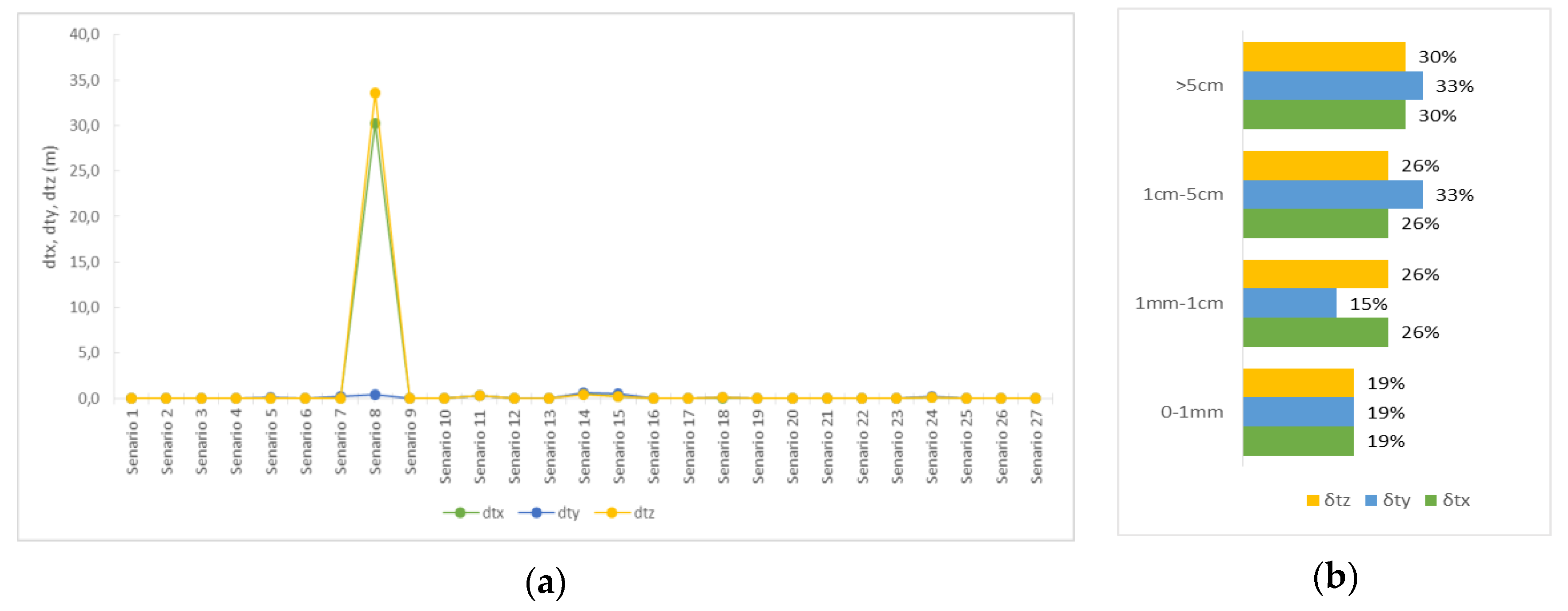
Finally, in the dual-quaternion method, the correct resolution percentage reached 93%, higher than the previous two methods. The failures were very small in scale, rotation, and translation. More specifically, the correct resolution percentages ranged from 93% to 96% for each case.

Regarding the translation, these were calculated with significant deviations in only two of the 27 scenarios, and specifically in scenarios 8 and 14. These showed deviations of 35 m and 65 cm, respectively. Figure 7 provides detailed data for each scenario and were found to be significantly larger, for the most part, compared to the previous two methods. This may be due to the fact that the transfers were recalculated using two quaternions, while they were not corrected during the main calculations, as in the previous cases. Respectively, their uncertainty depends on the uncertainty of the two quaternions with it ranging from a few tenths of a millimeter up to 6 cm.

Regarding the deviations of the scale, these were very small, of the order of ${10}^{-6}$ to ${10}^{-2}$ with an uncertainty of the order of ${10}^{-6}$. In this parameter, scenario 8 showed a maximum difference from the actual value equal to 1.13.

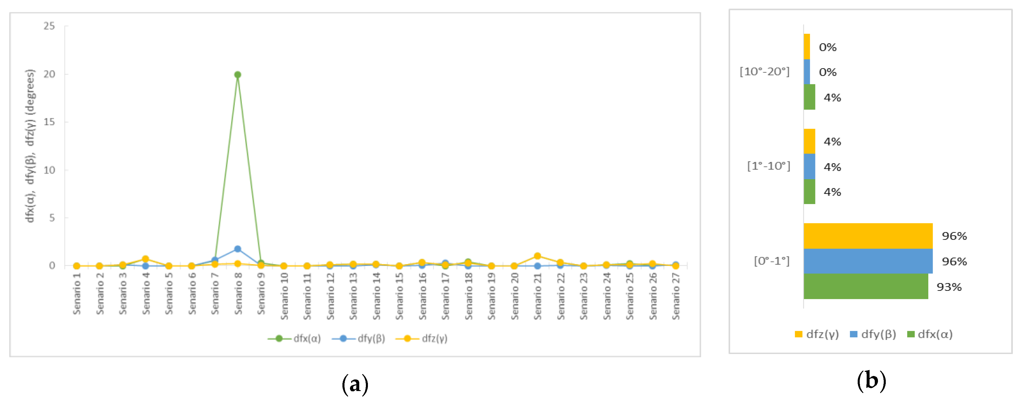
Finally, in terms of the angles’ solution, it had negligible differences in the majority. As shown in Figure 8, scenario 8 showed the greatest difference with the actual value, while deviations were also 1° in scenario 21. It is worth noting that this method has been proven to be the most effective for determining the rotation angles by calculating the two quaternions with one depending on the other, so their correct solution is “sealed”.

5. Testing Real Data

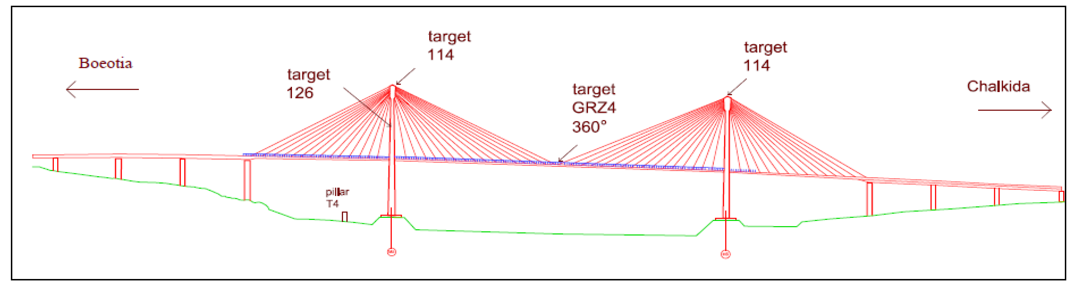
In order to understand the differences between each method, a real geodetic problem was tested. A well-known field of application of coordinate transformations is the monitoring of constructions for deformation testing. In this manuscript, a set of monitoring data of the Evripos Bridge, which connects Boeotia with Chalkida in Greece, as shown in Figure 9, is presented. [19]

5.1. Preparing the Dataset

The point dataset is in a local reference system. However, for convenience, it should be transformed into a system where the x-axis coincides with the longitudinal axis of the bridge, the y-axis coincides with the transverse axis of the bridge, and finally the z-axis coincides with the vertical axis of the bridge. After the calculations, the transformation parameters are shown in

Table 2. Transformation parameters for monitoring the Evripos Bridge in Greece.

	Translation (m)			Rotation (Degrees)			Scale Factor
	tx	ty	ty	fx(α)	fy(β)	fz(γ)	λ
Value	790.727	−371.595	0	0	0	51.41556	1
Uncertainty	±0.007	±0.007	0	0	0	6.7 · 10−7	0

.

In this paper, it is important to test the reverse problem for the 10 points presented before transformation in

Table 3. Tested points before transferred in the bridge system.

x (m)	y (m)	z (m)	σx (mm)	σy (mm)	σz (mm)
687.253	635.421	91.748	±5	±5	±5
687.253	635.421	91.748	±5	±5	±5
687.254	635.423	91.749	±5	±5	±5
687.252	635.422	91.749	±5	±5	±5
687.253	635.422	91.748	±5	±5	±5
687.253	635.421	91.748	±5	±5	±5
687.252	635.421	91.747	±5	±5	±5
687.255	635.423	91.748	±5	±5	±5
687.253	635.422	91.748	±5	±5	±5
687.254	635.423	91.748	±5	±5	±5

. Transformation parameters were used to have known points in both systems. However, the transformation parameters were calculated again from the points using the least square method to test the main deviations and their errors statistically.

The points’ accuracy before the transformation was ±5 mm for all coordinates x, y, z. After the transformation, considering the uncertainty of the transformation parameters, the accuracy was ±9 mm for x and y and ±5 mm for z. The rotation sequence was x–y–z and the least square method, that was used is as described above.

5.2. Results for Each Method

After solving for each method, a statistical analysis took place again. The deviations for each parameter were calculated and the uncertainty was tested.

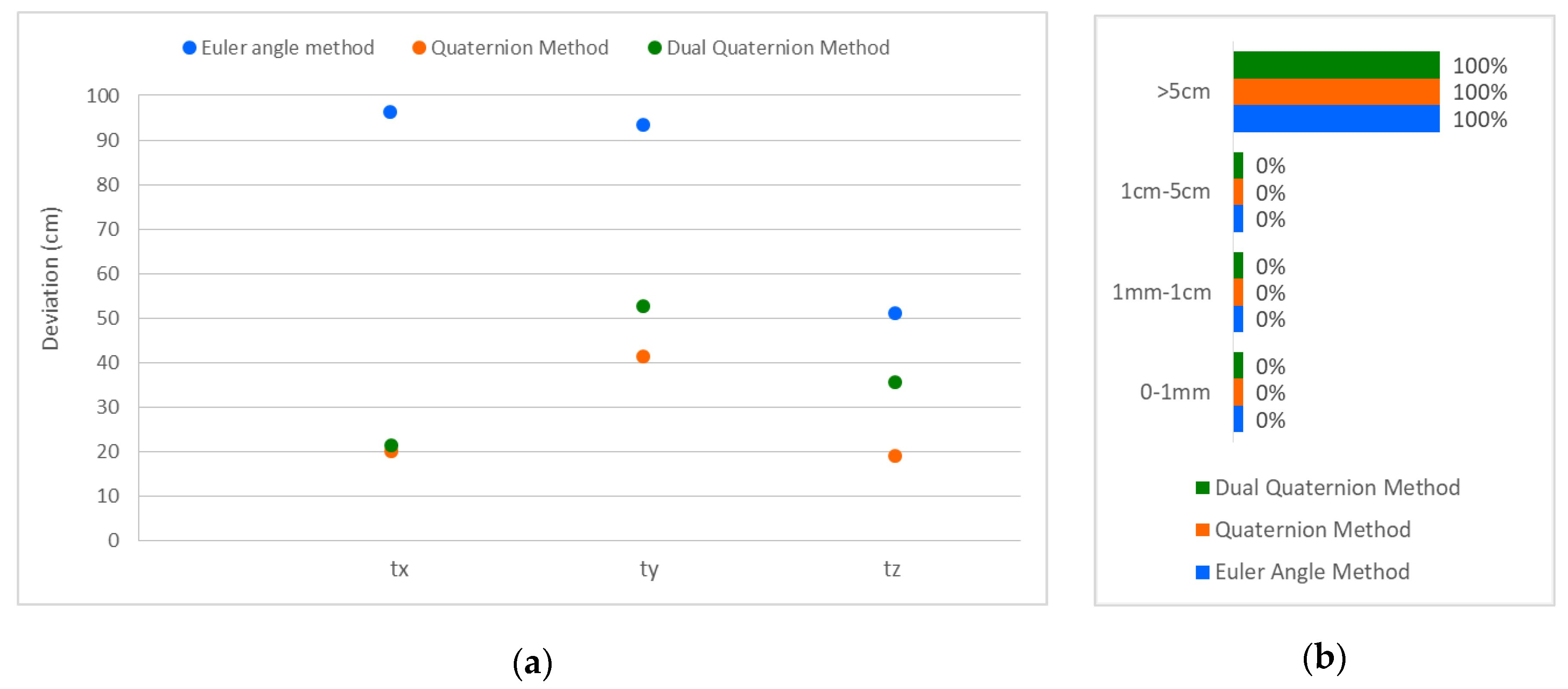
First, at all three methods, the translation parameters had significant deviations, which were from almost 20 to 95 cm. In Figure 10, in the majority, the quaternion method had the smallest deviations, rather than the Euler angle, which had the largest. Regarding the uncertainty, this was 2–3 mm in the Euler angle method, 5 cm in the quaternion method, and of the order of ${10}^{-5}$ at the dual-quaternion method.

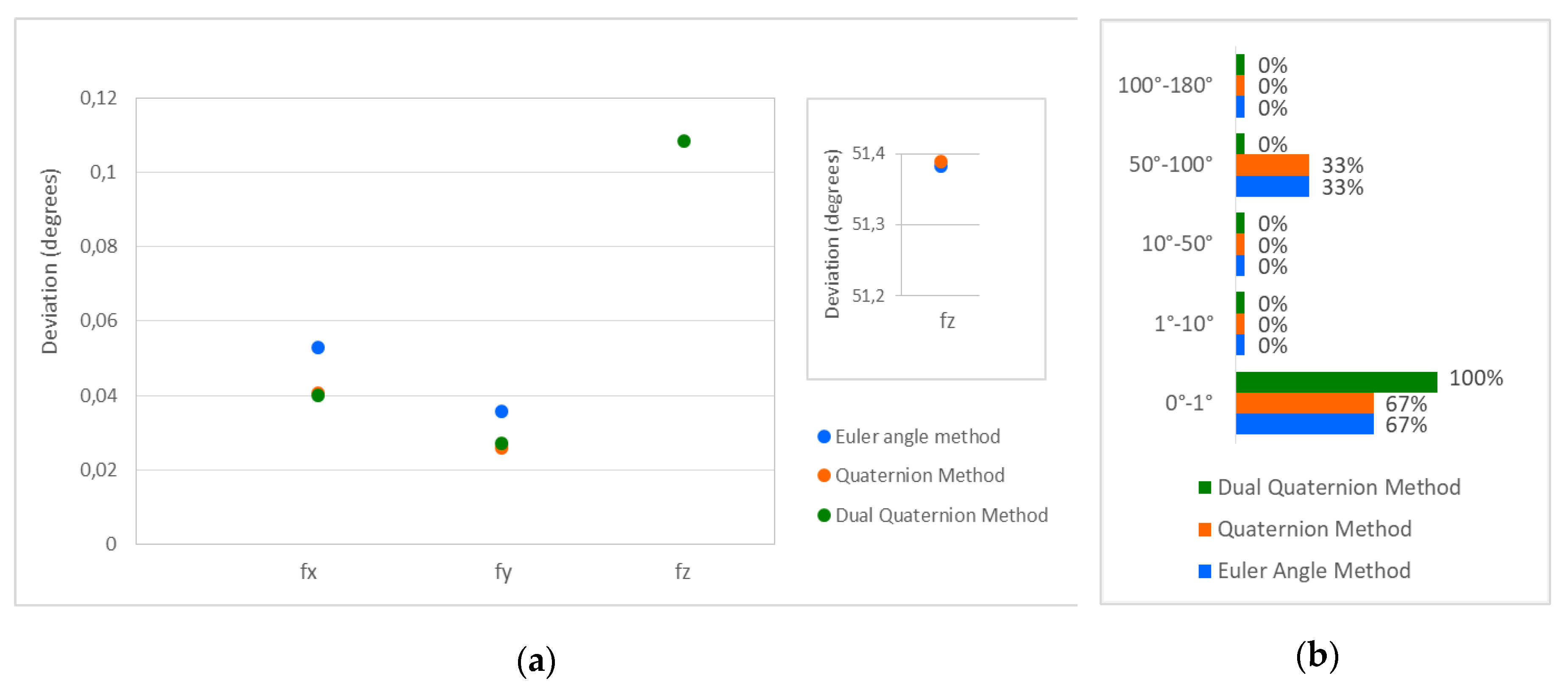
Considering the rotation angles, only the dual-quaternion method came close to calculating the correct values of each angle. In this way, 100% of the rotation parameters had deviations under 1°. According to Figure 11, the deviations at the Euler angle and quaternion method were almost the same and took values from 0° to 52°. Only 67% had deviations under 1°. For the uncertainty, the Euler angle method had an uncertainty less than 2″ and in the quaternion method was of the order of 2′ or less. Finally, in the dual-quaternion method, the uncertainty took values less than 1″ at all angles.

In conclusion, for the scale factor, every method had deviations equal to 0.0006 or less. The uncertainty was also small and took values under ${10}^{-6}$.

6. Discussion

The Helmert transformation problem or 7-parametric transformation in the reverse problem was performed in this paper. It is a three-dimensional transformation consisting of three turns between the axes that defines the rotation matrix (R), a vector of translation of their origins ($t_x,t_y,t_z$) as well as the uniform scale (λ) of one in relation to another. In order to calculate the transformation parameters, three different methods can be defined:

• The Euler angle method, where the Euler angles are used to define the rotation matrix, use the t-vector for translation, and use the scale factor λ for the scale.
• The quaternion method, where the rotation matrix is defined by the coefficients of a quaternion while here, the vector t for the transfer is also defined, and the coefficient λ for the scale.
• The dual-quaternion method, where the rotation matrix is defined by a quaternion, the transfer is given as a function of the quaternions of the rotation matrix and another quaternion, while the coefficient λ for the scale is also defined.

Taking into consideration the investigation of each method, for three different artificial datasets, it was found that the method of dual-quaternions produced the best values in the calculation of angles, while the other two methods optimized the values of the translation vector. Finally, the Euler angle method led to the correct solution of the scale for 100%.

Studying the scenarios for the whole data, it was found that for points that had small distances from each other, the method of dual-quaternion produced better results in the calculation of angles, while the method of quaternions resulted in a better transfer. In addition, for the second and third datasets, with large and medium distances between the points, respectively, small angle deviations existed in the dual-quaternion method, while the translations were better calculated in the Euler angle method.

Regarding the uncertainty of the calculated values, for the first dataset, the method of dual-quaternion produced values less than 1” for the angles and 1 mm for the transfers. Corresponding uncertainties were brought about by the Euler angle method in the angles and translations of the other two sets.

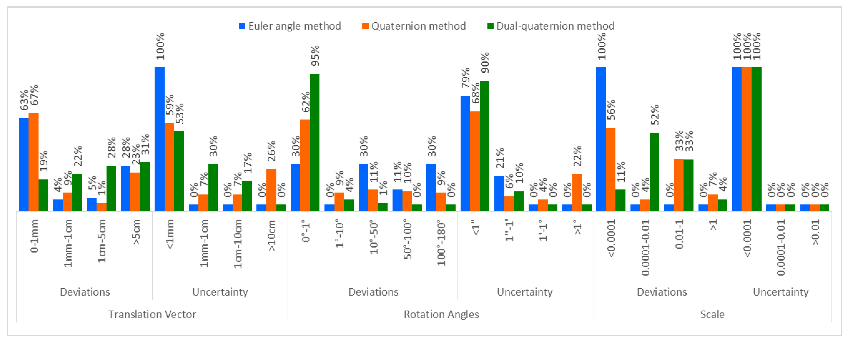
The analysis therefore shows that in order for a method to be fully satisfactory, it must have the smallest possible deviations with maximum accuracy. According to Figure 12 for the artificial scenarios and Figure 13 for the real data, this method does not exist to bring about the optimal solution in calculating angles, but also displacement and scale at the same time with great accuracy.

In the dual-quaternion method, finding the rotation angles is optimized to the fullest. This is because the dual-quaternion r of the turning matrix is also used to calculate the displacement, as a result of which it has a greater weight in the solution and thus “locks” its solution.

However, the same is not true of transfers. As above-mentioned, the coefficients $t_x,t_y,t_z$ of the translation vector in this method are not calculated individually, but occur as a combination of the two calculated quaternions. Thus, any error in their calculated values is transferred to the final transfer vector, resulting in an increase in its deviation from the actual value.

To sum up, after studying various scenarios, both real and artificial, it was found that the best way to determine the rotation was the dual-quaternion method, while it was not entirely clear which method optimized the translation. Locating the seven transformation parameters, it is proposed to investigate the improvement of the dual-quaternion method or create a new method that retains the elements for the angles, but optimizes those of the translation and scale.