Performance Evaluation of GIS-Based Artificial Intelligence Approaches for Landslide Susceptibility Modeling and Spatial Patterns Analysis

Abstract

The main purpose of this study was to apply the novel bivariate weights-of-evidence-based SysFor (SF) for landslide susceptibility mapping, and two machine learning techniques, namely the naïve Bayes (NB) and Radial basis function networks (RBFNetwork), as benchmark models. Firstly, by using aerial photos and geological field surveys, the 263 landslide locations in the study area were obtained. Next, the identified landslides were randomly classified according to the ratio of 70/30 to construct training data and validation models, respectively. Secondly, based on the landslide inventory map, combined with the geological and geomorphological characteristics of the study area, 14 affecting factors of the landslide were determined. The predictive ability of the selected factors was evaluated using the LSVM model. Using the WoE model, the relationship between landslides and affecting factors was analyzed by positive and negative correlation methods. The above three hybrid models were then used to map landslide susceptibility. Thirdly, the ROC curve and various statistical data (SE, 95% CI and MAE) were used to verify and compare the predictive power of the model. Compared with the other two models, the Sysfor model had a larger area under the curve (AUC) of 0.876 (training dataset) and 0.783 (validation dataset). Finally, by quantitatively comparing the susceptibility values of each pixel, the differences in spatial morphology of landslide susceptibility maps were compared, and the model was found to have limitations and effectiveness. The landslide susceptibility maps obtained by the three models are reasonable, and the landslide susceptibility maps generated by the SysFor model have the highest comprehensive performance. The results obtained in this paper can help local governments in land use planning, disaster reduction and environmental protection.

1. Introduction

Landslide is a sliding geological phenomenon of slope rock and soil mass moving along a shear failure surface. Landslides are natural disasters and existed before humans appeared. Now it has become an important global issue that threatens the safety of human life and property. There are many different scales of landslide occurrence in China every year. From January to July 2018, 1843 geological disasters were reported nationwide, including 973 landslides. The disasters caused the deaths of 74 people and a direct economic loss of CNY 1.04 billion. With the acceleration of urbanization in mountainous areas, the occurrence of landslides has increased and the threat to human life and property has also increased. Therefore, related risks need to be considered and evaluated. This requires researchers not only to study the inducing factors of landslides, but also to predict the spatial and temporal distribution characteristics of landslides. Due to many factors that induce landslides, such as lithology, rainfall, land use and human engineering activities, it is a challenging study to conduct spatial prediction research on the occurrence of landslides [1].

The role of the landslide susceptibility map (LSM) is to predict areas where future landslides may occur by studying areas where landslides occur and areas similar to those areas [2]. The identification of landslide susceptible areas is an important part of disaster management. For geologists, the landslide susceptibility map can be used as a good tool for disaster reduction and slope management [2]. Various factors control the reliability of landslide susceptibility maps, such as the quality and quantity of collected data, modeling methods, and accurate analysis [3]. Although a single model is widely used in landslide susceptibility assessment research, the study found that hybrid models obtained by combining different single methods in the same study area usually perform better in landslide susceptibility research. In addition, the applicability of the new models and methods should be further evaluated in different research areas, so as to obtain more accurate landslide susceptibility models and ensure that the landslide susceptibility maps made are more conducive to the research area for disaster management [4].

Over the years, scholars have undertaken a great deal of research into landslide hazard assessment [5,6]. In the rapid development of the geographic information system, today, appropriate integration processes and analyses can be performed for data collected from different sources using different methods. Logistic regression (LR) [7,8,9,10], certainty factor (CF) [11,12,13,14], weights of evidence (WoE) [15,16], evidential belief function (EBF) [17,18,19], and frequency ratio (FR) [19,20,21] methods were used to determine factors and their weights and produce landslide susceptibility maps. Nowadays, machine learning models have performed prominently in landslide susceptibility research, such as bagging [22,23], MultiBoost [24,25], naïve Bayes (NB) [26,27,28], Random forest [29,30,31], support vector machine (SVM) [12,32,33], logistic model trees [1,34,35] and boosted decision trees [36,37].

In this paper, landslide susceptibility mapping was carried out for Zichang County, China. Three machine learning methods, including the radial basis function network (RBFNetwork), naïve Bayes tree (NB), and SysFor (SF) models, were employed. Three models were used to establish the landslide susceptibility map, and then a more accurate landslide susceptibility map was obtained according to the results of different statistical methods.

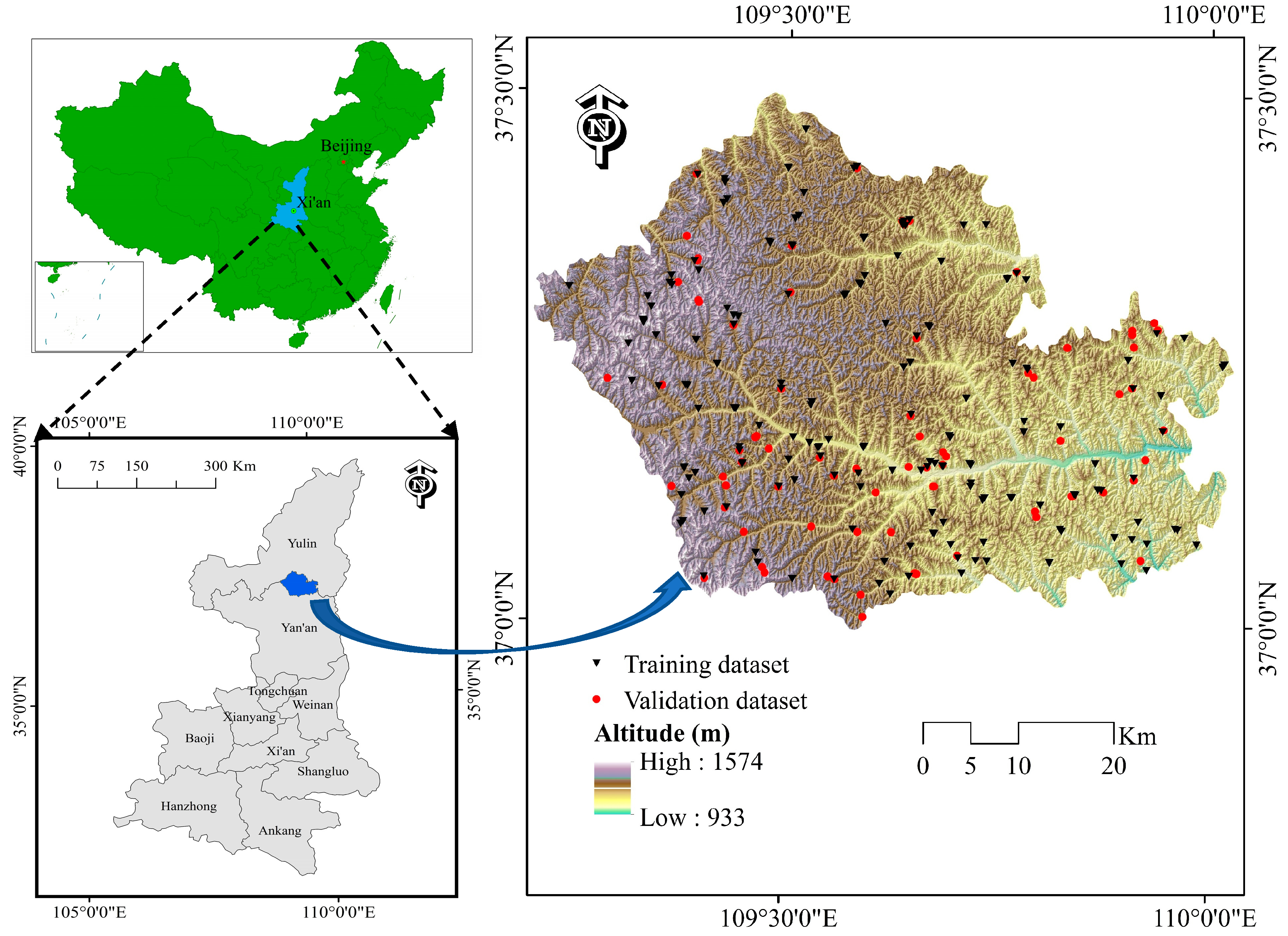
2. Geological and Geomorphological Setting

Zichang County is located within a longitude of 109°11′58′′E~110°01′22′′E and latitudes of 36°59′30′′N~37°30′00′′N (Figure 1). It belongs to the warm temperate semi-arid continental monsoon climate area with an annual average temperature of 9.1 °C and annual average precipitation of 514.7 mm. The study area has no obvious tectonic movements to transform it, and so it always maintains the characteristics of a stable sedimentary basin. The geomorphological types of the study area are more complicated. The soil and water loss around the beams and ridges are serious, accompanied by the development of a large number of landslides, collapses and other loess gravity landforms. The study area covers a variety of lithologies, such as loess, mudstone and sandstone, as shown in

Table 1. Geological formations.

Group	Lithology	Geologic Ages
A	Sandy gravel, loess-like silt	Quaternary
B	Malan loess, silty clay, sandy cobble	Quaternary
C	Lishi loess, silty clay, alluvium	Quaternary
D	Loess of Wucheng, silt interbedded with caliche nodule	Quaternary
E	Silt mudstone interbedded with calcium structure	Tertiary
F	Medium-coarse arkose	Cretaceous
G	Muddy limestone, shale siltstone interbedded	Jurassic
H	Sandstone, mudstone, argillaceous siltstone	Jurassic
I	Sandstone, shale and mudstone interbedded, pebbly sandstone, coal, oil	Jurassic
J	Mudstone sandy mudstone conglomerate, coal, oil, oil shale	Jurassic
K	Mudstone sandstone siltstone interbedded, coal	Triassic
L	Fine sandstone siltstone mudstone interbedded, oil	Triassic

.

3. Materials and Methods

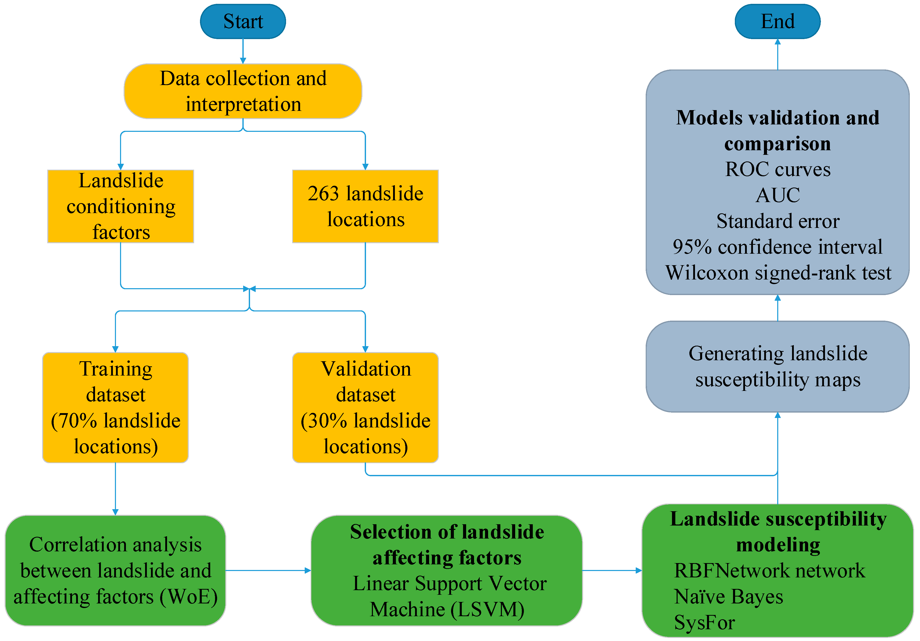
3.1. Methodology

The research method used in this paper can be divided into the following steps, as shown in Figure 2: (i) data collection; (ii) preparing the landslide conditioning factors and determining the landslide location; (iii) correlation analysis between landslide and affecting factors (WoE); (iv) selection of landslide affecting factors using the Linear Support Vector Machine (LSVM); (v) RBFN, NB and SF models are applied to assess landslide susceptibility in the study area; (vi) model validation and comparison; (vii) generating landslide susceptibility maps.

3.2. Preparation of Training and Validation Datasets

Landslide inventory and mapping is the foundation of landslide susceptibility mapping. In this study, the landslide survey data come from the following three methods: consulting the geological report of the study area; conducting a field survey with the help of the global positioning system (GPS); analyzing remote sensing images [38]. Finally, 263 landslides were identified in the study area, as shown in Figure 1. Rainfall and human engineering activities (engineering construction, urban construction and construction of highways and railways, etc.) are the main triggers of landslides [39], and loess landslide is the dominant type of landslide in the study area. Based on the analysis under GIS environment, the largest landslide in the study area is greater than 1 × 10⁷ m³, and the smallest landslide is close to 120 m³. Each landslide polygon in the data set was expressed using the centroid. Furthermore, it is necessary to randomly select the same number of non-landslide points in the study area—defining 263 landslide pixels as “1”, and then defining 263 non-landslide pixels as “0”. In this study, the original data were randomly divided into training data set and validation data set with the ratio of 70/30, because today there is no uniform specification for the division of the data set in LSM [1,40].

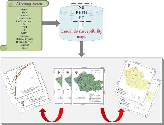
3.3. Landslide Affecting Factors

When the landslide inventory is compiled, the next step is to select landslide-affecting factors. The principles to be considered in the selection of conditioning factors are the characteristics of the geological environment and the data availability in the area [41,42,43]. According to the relevant literature [44,45,46], 14 landslide affecting factors were selected, including altitude, profile curvature, plan curvature, aspect, slope, SPI, TWI, STI, distance to rivers, distance to roads, lithology, soil, land-use and NDVI, as shown in Figure S1. The lithology map was extracted from geological maps with a scale of 1:200,000, the land use map was extracted from land-use maps with a scale of 1:100,000, the soil map was extracted from soil type maps with a scale of 1:1,000,000 and NDVI was produced using the Landsat 8 operational land imager. The remaining 11 factors were derived from ASTER GDEM with 30m resolution. Finally, all factors are eventually converted to the same resolution (30 × 30 m).

The establishment of the altitude maps is the first step in conducting research. In the study area, it is divided into seven levels according to the interval of 100 m: (1) 933–1000; (2) 1000–1100; (3) 1100–1200; (4) 1200–1300; (5) 1300–1400; (6) 1400–1500; (7) 1500–1574. The profile curvature reflects the rate of change of the surface elevation at the maximum slope of the surface. This study calculated the profile curvatures in ArcGIS software and divided them into five categories: −7.29 to −1.65; (2) −1.65 to −0.46; (3) −0.46 to 0.58; (4) 0.58 to 1.97; (5) 1.97–9.45. This study calculated the plan curvatures in ArcGIS software and divided them into five categories: (1) −9.24 to −1.79; (2) −1.79 to −0.54; (3) −0.54 to −0.38; (4) −0.38 to 1.43; (5) 1.43–7.56. Aspect is an important factor for landslide susceptibility maps [47,48,49,50]. The aspect layer was divided into nine classes: (1) Flat; (2) North; (3) Northeast; (4) East; (5) Southeast; (6) South; (7) Southwest; (8) West; (9) Northwest. The slope angle is directly related to the study of the landslide and is an indispensable factor in the preparation of the landslide susceptibility map [51]. The slope in the study area can be divided into six categories: (1) < 10; (2) 10–20; (3) 20–30; (4) 30–40; (5) 40–50; (6) > 50.

The stream power index (SPI) refers to the erosion of flowing water, the thickness of the soil layer and the content of sand and silt. SPI has been widely used in the study of landslide susceptibility [52]. These factors will affect the occurrence of slope damage events [53]. SPI has the following formula:

$$SPI=As\tan B$$

(1)

where As represents a specific catchment area and B represents a local slope [53]. According to the calculated value, the SPI is grouped into five categories: (1) < 10; (2) 10–20; (3) 20–30; (4) 30–40; (5) > 40.

The topographic wetness index (TWI) can reflect the moisture content in the soil. TWI can be expressed by the formula [54]

$$TWI=\ln (\frac{\partial }{\tan B})$$

(2)

where ∂ is a local uphill contribution area representing the amount of water flowing to a particular location and tan B is a local slope. The TWI map of the study area consisted of the following six categories: (1) 1.11–2; (2) 2–3; (3) 3–4; (4) 4–5; (5) > 5.

The sediment transport index (STI) value represents the degree of land current erosion and sedimentation [55]. According to the value of STI, it was divided into five categories: (1) 0–10; (2) 10–20; (3) 20–30; (4) 30–40; (5) > 40.

The distance to rivers map was divided with five different buffer ranges including: (1) 0–200; (2) 200–400; (3) 400–600; (4) 600–800; (5) > 800. The relationship between the river and the landslide can be established through these buffer zones [55,56,57]. The distance to roads was used as a landslide-affecting factor because the road repaired near the slopes reduces the load on the terrain and the heel of the slope [51]. We calculated the pavement buffer every 100 m in the study area: (1) 0–100; (2) 100 –200; (3) 200–300; (4) 300–400; (5) > 400.

Different lithology units have a different magnetic susceptibility [58,59]. A total of five lithologic units are in the study area: Quaternary, Tertiary and Cretaceous, Jurassic and Triassic. The soil in the soil map can be divided into five categories: alluvial soils; red clay soils; lakes and reservoirs; cultivated loess soils; all other values.

The main land-use of the study area is farmland, forestland, grassland and water bodies, residential areas and others. The NDVI can accurately reflect the surface vegetation coverage. The data come from satellite remote sensing images. In this study, this can be classified as: (1) 0.15–0.01; (2) 0.01–0.04; (3) 0.04–0.07; (4) 0.07–0.09; (5) 0.09–0.31.

3.4. Weights of Evidence

The weights-of-evidence model is built from the logarithmic form of Bayes’ rule. The weighted values for the classes of landslide-affected factors can be written as in Equations (3) and (4) [60]:

$$W^{+}=\frac{\frac{P_1}{P_1+P_2}}{\frac{P_3}{P_3+P_4}}$$

(3)

$$W^{-}=\frac{\frac{P_2}{P_1+P_2}}{\frac{P_4}{P_3+P_4}}$$

(4)

where P1 and P2, respectively, represent the number of pixels that appear and do not appear in the same given factor category. P3 represents the number of pixels that have no landslides in a particular factor category. When there is neither a landslide nor a landslide pixel in a particular factor category, P4 is used [61].

The positive weight (W +) not only indicates that the affecting factors leading to landslides exist, but also that the value reflects the positive correlation between the factors and landslides. The negative weight (W-) reflects the degree of negative correlation between them [60]. The difference between the two weights can be expressed as Equation (5):

$$C=W_i^{+}-W_i^{-}$$

(5)

where C is the weight contrast. According to the value of C, the relationship between predictor variables and landslides can be reflected more comprehensively.

3.5. Naïve Bayes

The model can be built by following a few steps: (i) collect examples; (ii) estimate the prior probability of each class; (iii) estimate the mean of the class; (iv) construct a covariance matrix and find the inverse and determinant for each class; (v) for each class formation, create a discriminant function [62]. The unique point of this model is that only a small amount of training data is required for evaluation and analysis to obtain the parameters required for classification [62]. More importantly, building a model is simple [63]. The NB method is widely and successfully used in landslide susceptibility evaluation research [12,32,64].

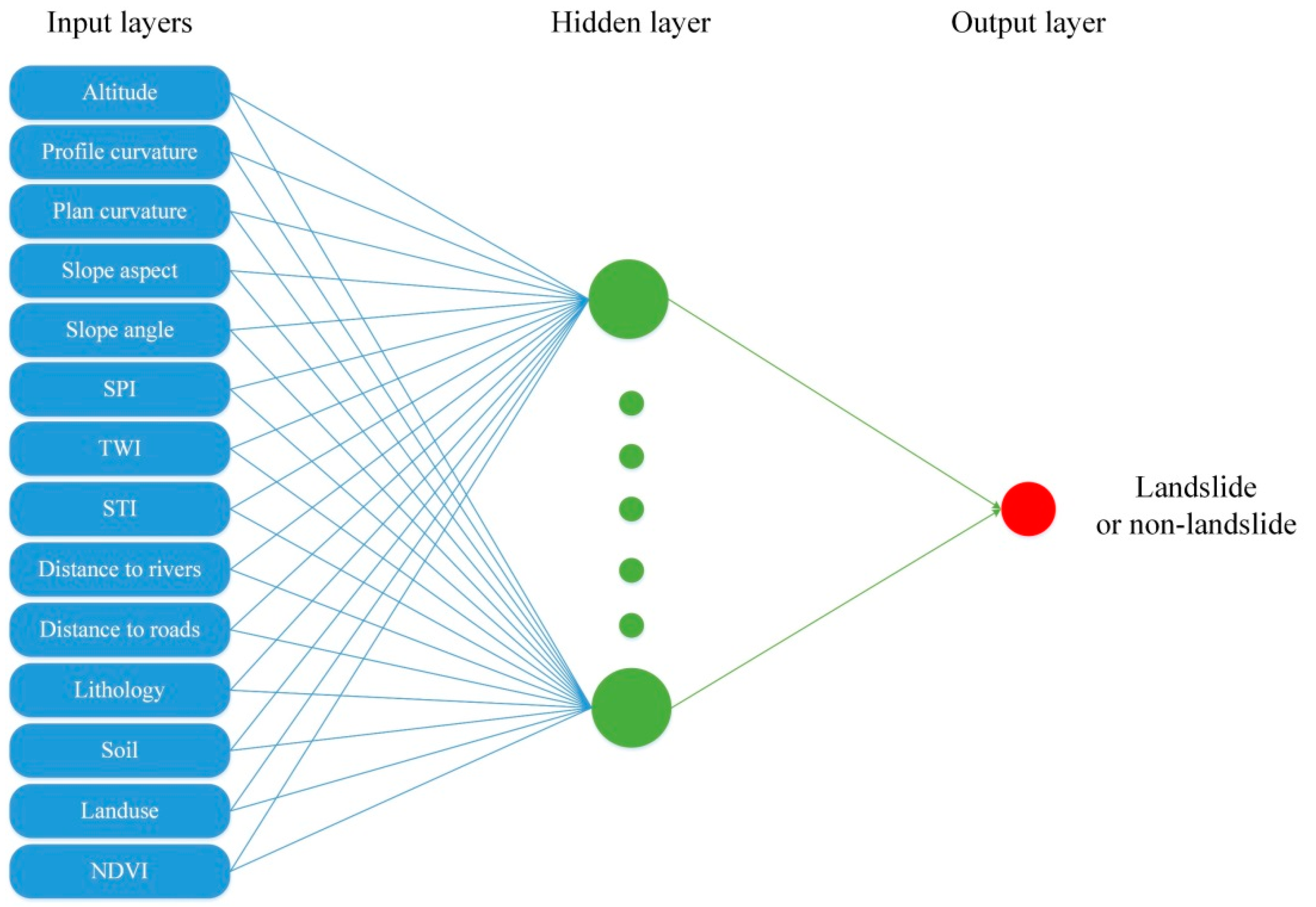
3.6. Radial Basis Function Network

The radial basis function (RBF) originates from solving the multivariate interpolation problem. Later RBF networks were used in other programs [65,66]. The RBF network model is based on an algorithm from K-means clustering [67]. The essence of the RBF network is a radial function. It provides convenience in solving non-linear problems [68]. First, the data are imported into the input layer without calculation and then the nonlinear problem of the hidden layer neuron is processed and sent to the linear output layer. There is only one hidden layer in the RBF network itself, but there is no hidden layer in the model [69]. The hidden layer can be activated by a function, f: Rn→R, if properly trained. Typically, the basis function commonly used in RBF networks is the Gauss function.

For all the possible choices for f, the Gaussian function can be written as:

$$f_i(\mathrm{x})=f_i({\mathrm{e}}^{\frac{-\left|\right|x_{\mathrm{p}}-{\mathrm{c}}_{\mathrm{i}}\left|\right|}{d_i}}),\mathrm{i}=1,2,....,\mathrm{n}$$

(6)

$$Y=W^T{f}_p$$

(7)

where C_i ∈ Rn indicates the center of the basis function. There are n hidden layer nodes. Let f_i d_i ∈ R be the radius of the first hidden layer node. Through the weight matrix (W ∈ Rn_i × n) to connect the hidden layer nodes and network output, f_p is the hidden node vector.

3.7. SysFor

SysFor is built for a great many good quality decision trees by both low-dimensional and high-dimensional datasets and is applied to many applications [70]. A SysFor can be built by following a few steps: (i) follow the user’s instructions to find a set of “good properties” and corresponding split points; (ii) build the number of trees based on good attributes and user definitions; (iii) take the level 1 node of the tree built from step 2 and select an optional good attribute from the set of good attribute; (iv) return all the trees built in steps 2 and 3 as Sysfor [71].

This technique can be used to study a data set and master the mode of recording for the purpose of classifying a record as one of “class values”. Importantly, the model can predict the “class value” of an unknown tag. The model functions similar to decision trees and decision forests [72].

3.8. Support Vector Machine

The quality of the selected model and input data will affect the quality of landslide susceptibility assessment [73]. Using this method to test the affecting factor can be expressed as (Equation (8)):

$$g\left(x\right)=\mathrm{sgn}\left(w^{T}a+b\right)$$

(8)

where w^T represents an inverse matrix, the weight matrix of each landslide affecting factor in this study, a = (a1, a2, …, a14) is the input vector (14 landslide-affecting factors) and b is the offset from the origin of the hyperplane. The closer the weight w_i is to 0, the less important the landslide-affecting factors are to the prediction of landslides [74].

4. Results and Analysis

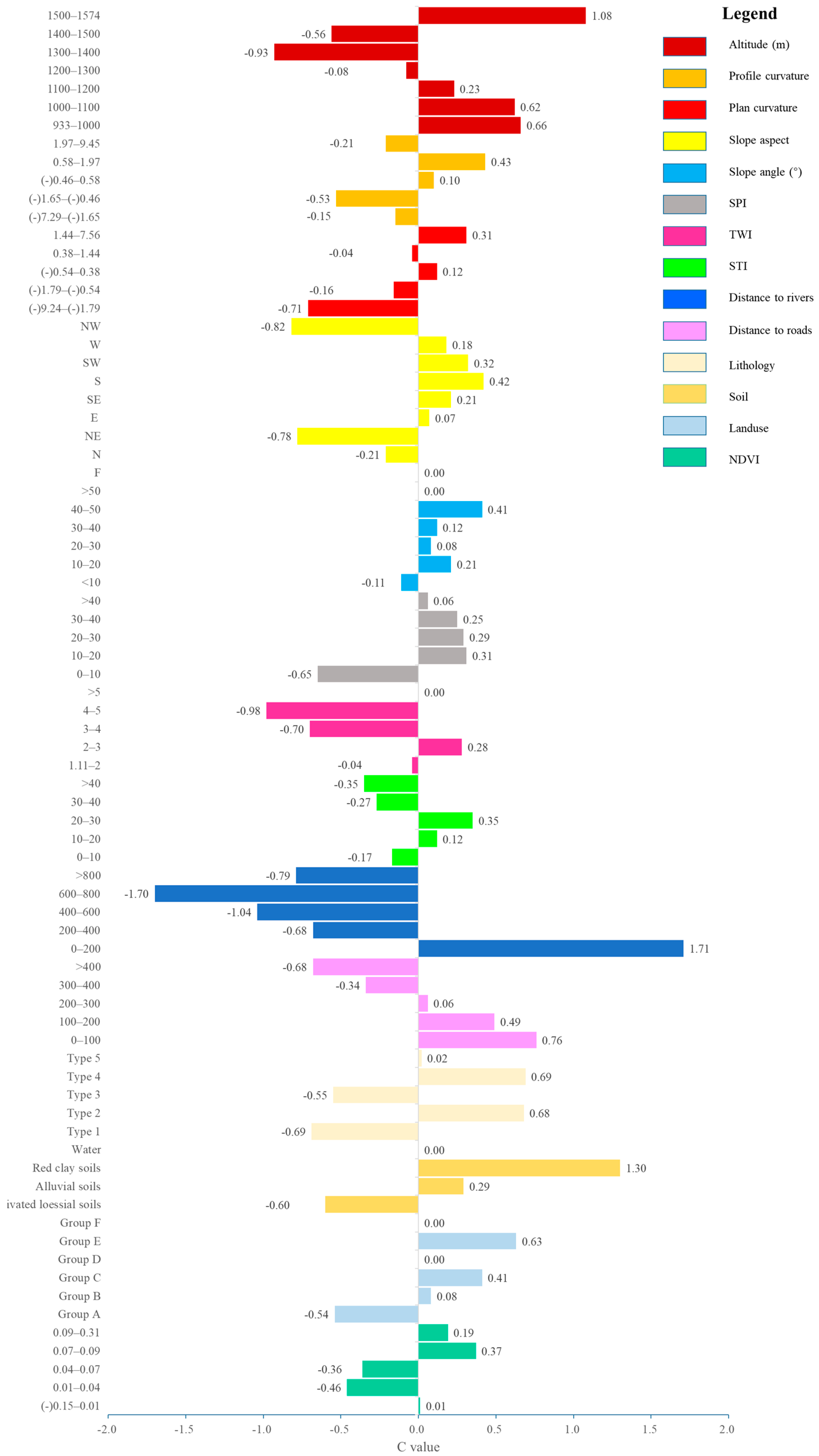
4.1. Correlation Analysis of Affecting Factors

In this paper, the WoE model is used to analyze the correlation between landslide occurrence and affecting factors, as shown in Figure 3. The overall spatial correlation between the predictable variable and the landslide can be reflected by C. WoE results analysis, which showed that the correlation with the landslide decreased with the increase in elevation. An increase in altitude is accompanied by an increase in precipitation, a decrease in temperature, and accelerated weathering, thereby promoting the occurrence of landslides [75]. Therefore, an altitude >1500m had the highest correlation compared with other elevation ranges. In terms of profile curvature, it was only positively correlated with the occurrence of landslides at (−0.46 to 0.58) and (0.58–1.97), and 42% and 29% of landslides occurred at the two profile curvature points. The plan curvature is positively correlated with the occurrence of landslides in the range from (−0.54) to 0.38 and from 1.44 to 7.56, and negatively correlated in other ranges. Both the profile curvature and the plan curvature control the speed of flowing water affect the degree of slope erosion [76]. If the slope direction is different, then the slope surface is different from the sun exposure and rainfall erosion, resulting in different slope materials [50]. In the southern part, 15% of landslides occur, and the correlation is highest in this orientation with landslides. When the slope is <10° or >50°, the occurrence of the landslide is randomly distributed; the correlation with the landslide is the highest in the range of 10–20, and 30% of the landslides occur in this range, meaning that this affecting factor has a high incidence of landslides in this range. The SPI value has the highest correlation, with an occurrence of landslides in the range of 10–20.

Additionally, the C values for STI values in the range of 10–20 and 20–30 are 0.12 and 0.35, respectively, indicating that the landslides are predictable and positively correlated with the STI values. TWI is positively correlated with the occurrence of landslides only in the 2–3 range. The WoE results show that the correlation of this variable with landslides decreases with increasing distance to rivers, and the same results are also shown in the distance to road. The closer to the river, the stronger the erosion at the bottom of the slope, which affects the slope stability [51]. At the same time, building roads changes the original stability of the terrain [15]. Different lithologic units have different compositions and structures, etc., and thus produce different capabilities regarding resistance to landslide occurrence [77]. The WoE analysis of the lithology in the study area revealed that Tertiary, Jurassic and Triassic were positively correlated with the occurrence of landslides. The relationship between land use and slope stability is that different types of land-use will produce different vegetation, and the roots of different vegetation will help maintain the stability of the slope differently [78]. When the soil is alluvial soil and red clay soils, it is positively correlated with the occurrence of landslides. In land-use, 54% of landslides occur in Group C and are positively correlated with landslides in this region. However, the highest correlation is in Group E. Finally, WoE finds that the NDVI value has the highest positive correlation with the occurrence of a landslide in the range of 0.07–0.09 and the highest negative correlation in the range of 0.01–0.04.

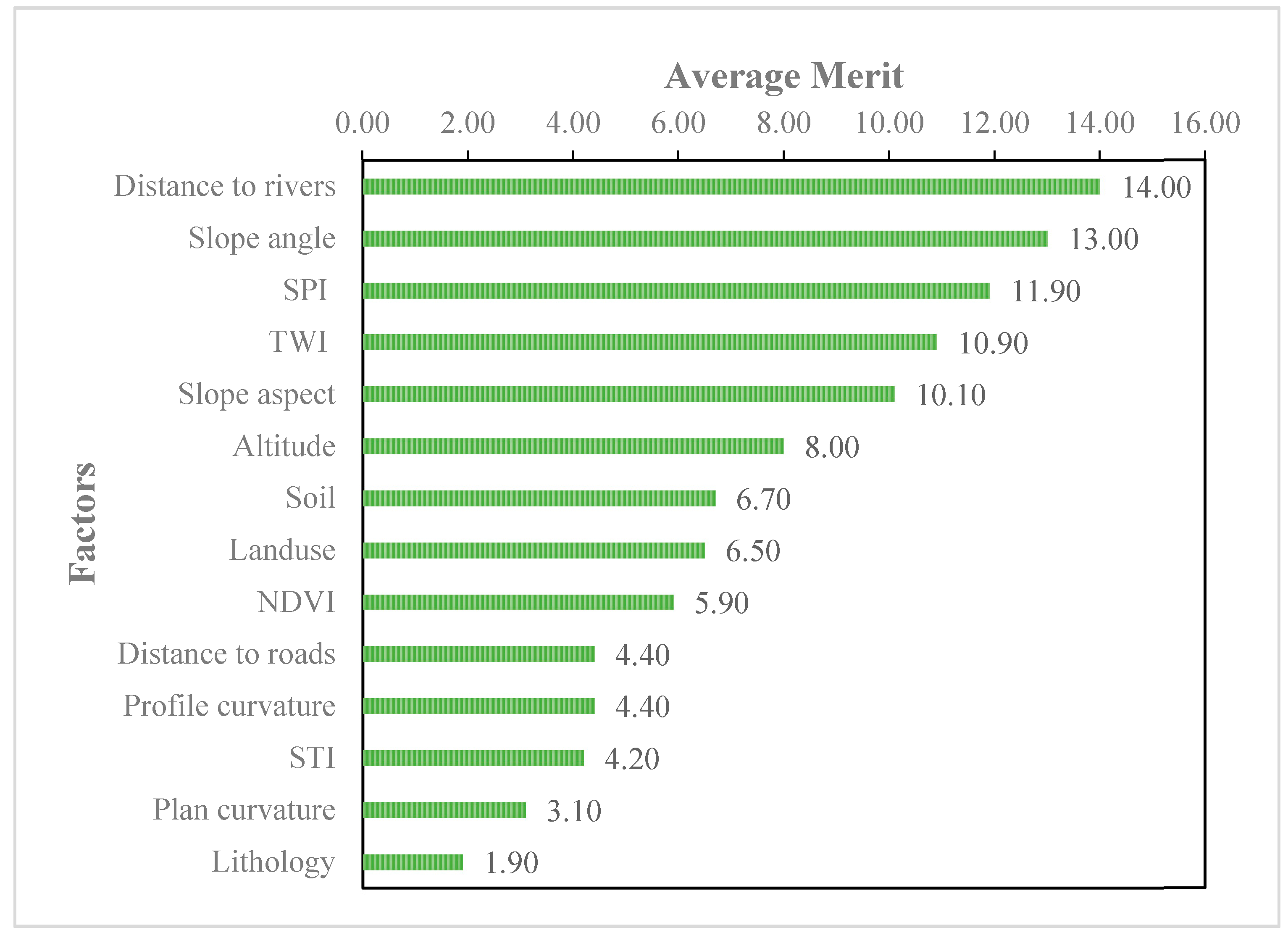
4.2. Selection of Landslide-Affecting Factors

The prediction ability evaluation and comparison of 14 landslide impact factors show that, although the contribution of each factor is different, they contribute to landslide prediction modelling, as shown in Figure 4. The result shows that distance to rivers has the highest predictive capability (14), followed by slope angle (13), SPI (11.9), TWI (10.9), slope aspect (10.1), altitude (8), soil (6.7), land-use (6.5), NDVI (5.9), distance to roads (4.4), profile curvature (4.4), STI (4.2), plan curvature (3.1) and lithology (1.9). Therefore, all 14 affecting factors were selected for the models.

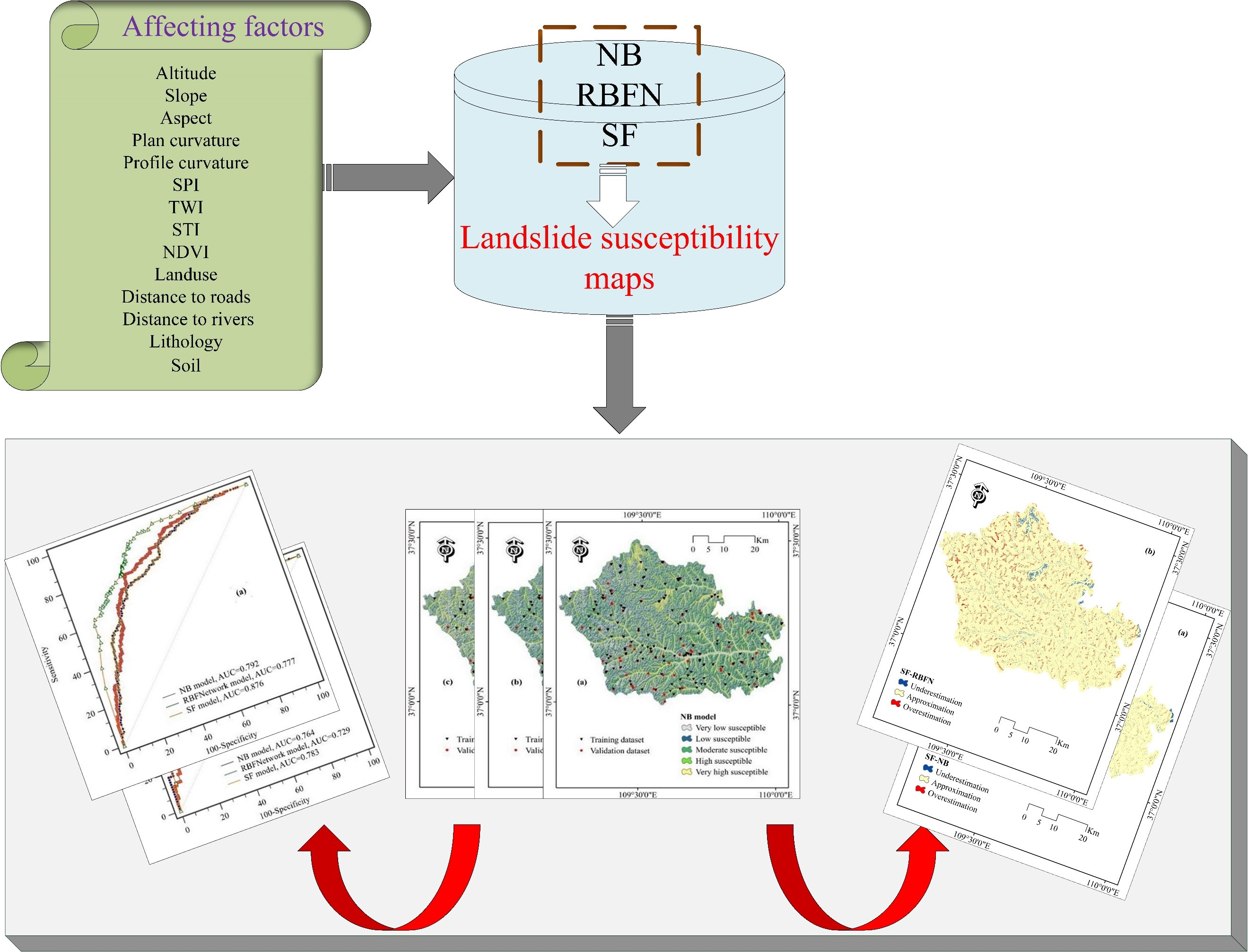
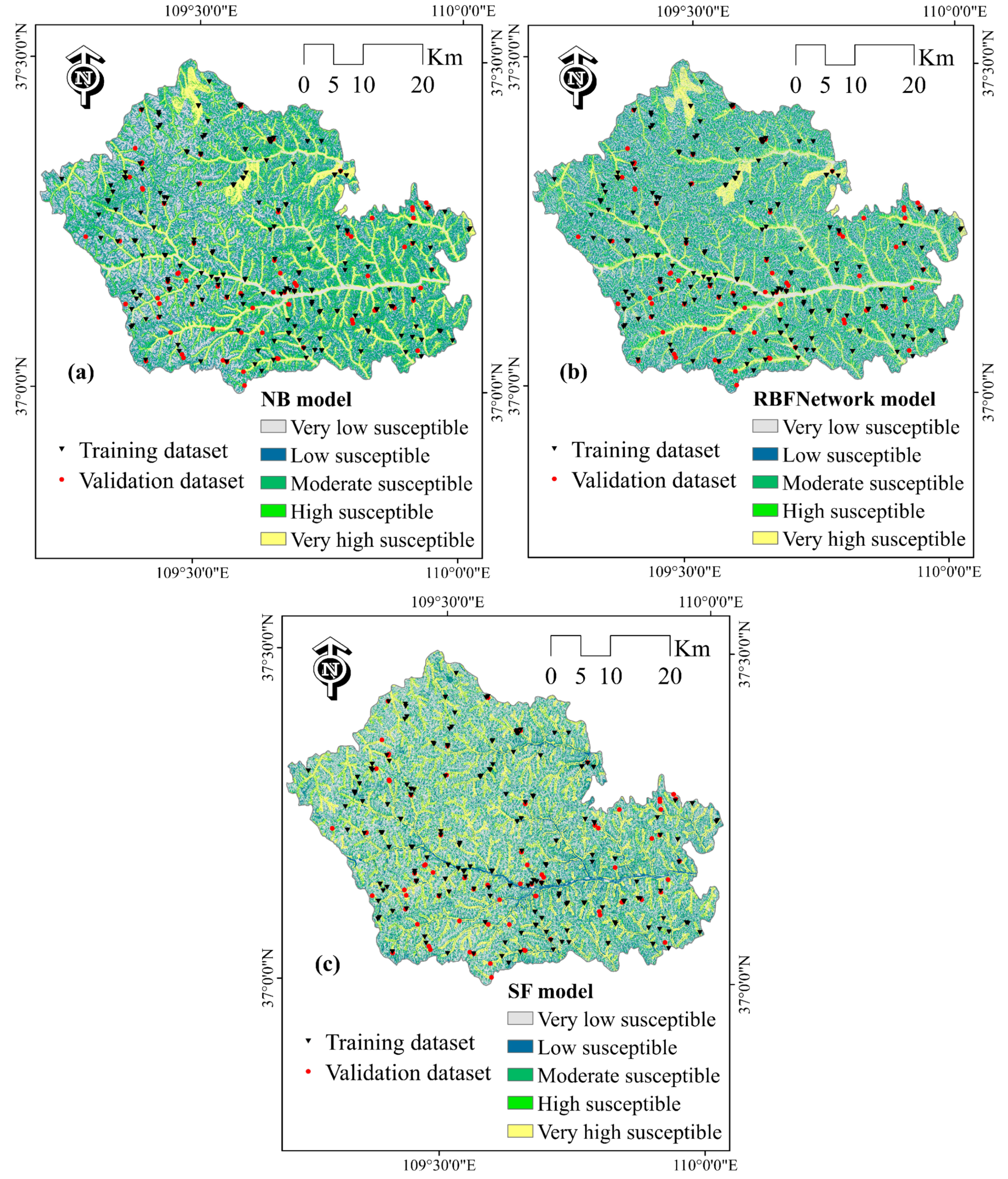
4.3. Constructing Landslide Susceptibility Maps

Generating the landslide susceptibility map generally requires the following two steps [38]: first, obtain the landslide susceptibility index (LSI) of all the evaluation units; then reorganize the LSI obtained in the first step. The specific operation is to calculate the LSI of each evaluation unit by using the probability distribution function of the evaluation model and then re-divide the obtained LSI by the natural discontinuous point grading method in the ArcGIS software. In this study, NB, RBFNetwork and Sysfor models generated three landslide susceptibility maps, as shown in Figure 5. Figure 5a is the landslide susceptibility mapping generated by the NB model. The LSI is divided into five ranges of 0–0.133, 0.133–0.322, 0.322–0.537, 0.537–0.769, and 0.769–1. Figure 6 shows that the very low level has the largest area.

Figure 5b is the landslide susceptibility mapping generated by the RBFNetwork model, and the landslide susceptibility categories were also divided into five categories. The LSI is divided into five ranges of 0.203–0.288, 0.288–0.407, 0.407–0.543, 0.543–0.721 and 0.721–0.88, as shown in Figure 6. In this study, the structure of the network consists of three layers: an input layer of 14 neurons; a hidden layer (called an RBF unit); an output layer containing a neuron, as shown in Figure 7. The learning process of the RBFNetwork can be divided into two parts: (a) using the K-means algorithm to calculate the number of clusters (hidden neurons); (b) the optimal estimation of kernel parameters [1].

The SysFor model should be optimized before generating a landslide susceptibility map. The best parameters for the SysFor model were found through testing—the confidence was 0.1 and the numberTrees value was 60. Figure 5c is the landslide susceptibility mapping generated by the SysFor model, and the LSI is also divided into five categories. The LSI is divided into five ranges of 0–0.114, 0.114–0.314, 0.314–0.549, 0.549–0.78 and 0.78–1. Figure 6 shows that the very low level has the largest area.

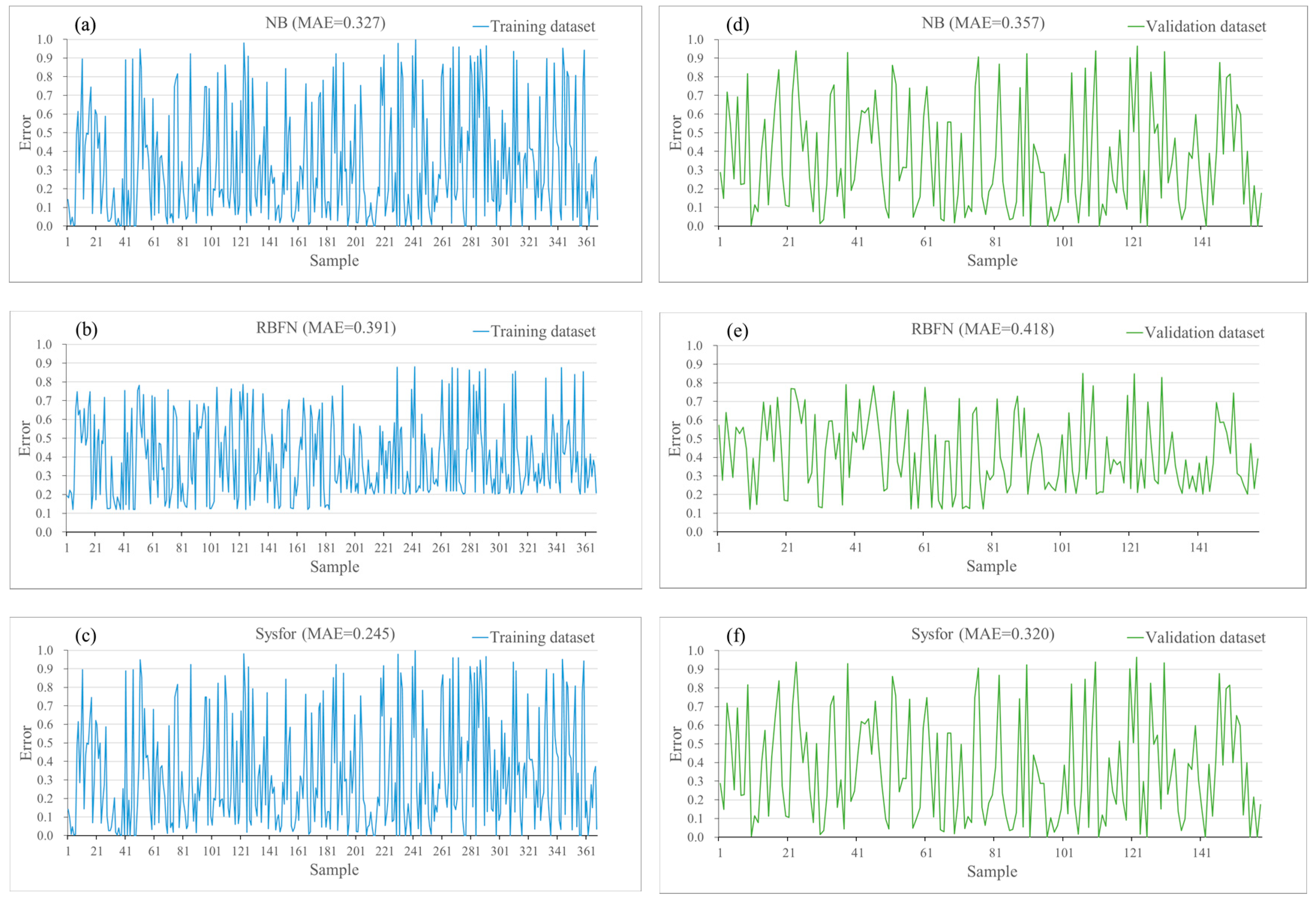
4.4. Models Validation and Comparison

The landslide susceptibility map is the most direct and authoritative evidence to test the performance of the landslide susceptibility model [79]. Without model validation, the establishment of landslide susceptibility maps has no practical significance [24]. Therefore, the receiver operating characteristic (ROC) curve and the area under the curves (AUC) [80,81] are used to evaluate the predictive power of each model.

Figure 8a and

Table 2. Parameters of ROC curves with the training dataset. CI: confidence interval.

Variable	AUC	SE	95% CI
NB model	0.792	0.0233	0.746 to 0.832
RBFNetwork model	0.777	0.0240	0.731 to 0.818
SF model	0.876	0.0174	0.838 to 0.908

show the ROC curve and its parameters under the training data set, respectively. Under the training data set, the areas under the NB and Sysfor model curves were 0.792 (79.2%), 0.777 (77.7%) and 0.876 (87.6%), respectively. Figure 8b and

Table 3. Parameters of ROC curves with the validation dataset.

Variable	AUC	SE	95% CI
NB model	0.764	0.0377	0.690 to 0.828
RBFNetwork model	0.729	0.0397	0.653 to 0.797
SF model	0.783	0.0360	0.710 to 0.844

show the ROC curve and its parameters under the validation data set, respectively. In the validation data set, the areas under the NB, RBFNetwork and Sysfor model curves were 0.764 (76.4%), 0.729 (72.9%) and 0.783 (78.3%), respectively. In addition, evaluation statistics (MAE) are used to verify the model. The mean absolute error (MAE) is a measure of the difference between two continuous variables (predicted and observed values). The SysFor model has the smallest MAE value under training data (MAE = 0.245) and validation data (MAE = 0.320), indicating that the model also performs well in the prediction and observation comparison of landslide occurrence, as shown in Figure 9.

The Wilcoxon signed-rank test was used to determine the significance of the differences between the susceptibility models, where the main determinants were p and z. The test is used to determine whether there is a significant difference in the susceptibility model—whether the p value is less than the significance level (0.05), and whether the z value is within the range of the critical value (−1.96, + 1.96) [1]. It can be seen from the analysis in

Table 4. Results of the Wilcoxon signed-rank test (two-tailed).

Pair-Wise Comparison	z-Value	p-Value	Significance
NB vs. RBF Network	1.081	0.280	No
NB vs. SF	5.677	0.000	Yes
RBFNetwork vs. SF	5.350	0.000	Yes

that the performance difference between the SF model and the other two models (RBFN and NB model) is statistically significant. In contrast, for the NB and RBFNetwork model, the performance difference was not statistically significant.

Comparing the performance rankings of the models obtained under the training data set and the validation data set, it can be found that the performances of the models under the two sets of data have the same ordering—the Sysfor model has the highest accuracy (0.783), followed by the NB model (0.764) and RBFNetwork model (0.729). Other statistical methods show that the Sysfor model has a minimum standard error (SE) and a 95% confidence interval (CI).

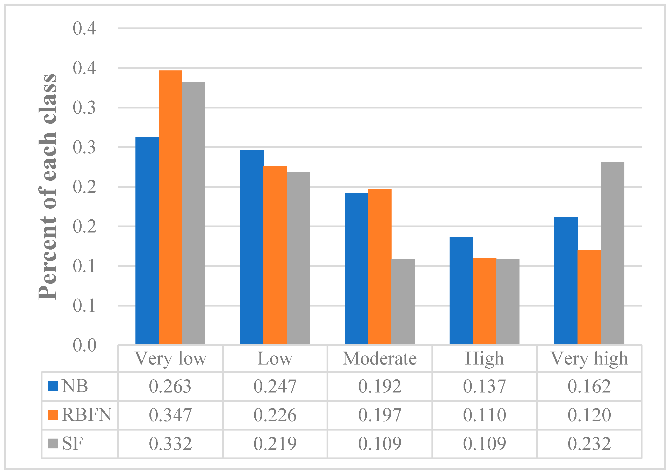
4.5. Comparison of Landslide Susceptibility Maps

In this study, SF model was selected as the benchmark model, and the susceptibility maps generated by the other two models were matched with the susceptibility maps generated by the SF model using the method developed by Xiao et al. [82]. The difference between them is defined by subtraction in ArcGIS, as shown in Figure S2. The raster values of the three susceptibility maps are between 0 and 1, so the value range of the comparison maps is (−1, 1). The three levels of underestimation, approximation and overestimation are based on the values obtained from the comparison map. Table S1 shows the percentages of different levels in the total area. The values of both comparison maps break at −0.50 and 0.50. To obtain the key factors that cause differences between susceptibility maps, it is necessary to associate overestimated and underestimated pixels with all the adjustment factors used in the susceptibility analysis. Underestimations and overestimations of each category of factors are counted, as shown in Tables S2 and S3. For each class, the ratio of each class to the total area is defined as A. The ratio of the underestimated pixels in the class to the total underestimated pixels is defined as B. “B–A”, as the ratio of the differences between the two maps, can be used to identify the key classes of underestimated anomalous clustering. The value of “B–A” can be used to determine the class with the highest degree of imbalance, as shown in

Table 5. Imbalanced class causing spatial distribution of underestimation and overestimation.

Classification	Comparison Maps	Imbalanced Classes
Underestimation	SF-NB	Red clay soils
	SF-RBFN	SPI, 10–20; Red clay soils
Overestimation	SF-NB	Distance to rivers, 0.200
	SF-RBFN	Distance to rivers, 0.200

. Figure S3 shows underestimations of “SF-NB” and “SF-RBFN” driven by red clay soils, underestimations of “SF-RBFN” driven by SPI. Figure S4 shows overestimations of “SF-NB” driven by distance to rivers, and overestimations of “SF-RBFN” driven by distance to rivers.

5. Discussion

The analysis of the weight values shows that natural factors are not the only factors affecting the occurrence of landslides, and the intensification of human activities and engineering construction may also affect the geological environments and occurrence of landslide disasters [83]. Landslide occurrence in Zichang County is the highest at the slope angle of 40–50, and when the slope angle is >50, the values of W+ and C are 0, supporting that prediction. Through the WoE analysis of the distance to roads, it is found that the closer the distance to roads, the larger the positive weight of W+, indicating that closeness to a road means that land is greatly affected by human activities, thus promoting the occurrence of landslides [84,85]. In general, the growth density of vegetation is inversely proportional to the possibility of a landslide, and land-use is of high importance for landslide susceptibility assessment [86,87]. Group C (Grassland) has a higher vegetation coverage than Group B (Forestland), so the correlation is higher than Group B. Each landslide-affecting factor contributes to the landslide susceptibility assessment, but each has its differences. Table 1 shows that 60% of the landslides occurred in the lithology type 1 (Quaternary loess), but the five groups in the study area lithology WoE analysis found in the region of the lithology for Type 1 had a poor correlation with the occurrence of landslides.

The three landslide susceptibility maps show similar landslide susceptible areas—especially the gullies on the study area. The study area is located in the middle of the Loess Plateau in northern Shaanxi. The cultivated loess soils cover almost the whole area. The special topography and geotechnical condition define the deformation and failure modes of the slopes and at the same time, they control the developmental characteristics of the landslide disasters, which determines the research. The area belongs to a high-incidence area of landslide disasters, which further reflects the importance of landslide susceptibility assessments in the study area [88].

After statistics, it is found that the number of overestimations and underestimations is limited (the overall discrepancies range from 0.04% of the total area in SF-NB to 0.07% in SF-RBFN). Through visual analysis, it is found that the distribution of overestimation and underestimation is not random, and a certain spatial pattern can be found on the comparison map. The existence of this spatial pattern may be due to a systematic error in the susceptibility analysis [82]. Such systematic errors indicate the finiteness and effectiveness of the model. Comparing the SF model as the benchmark model with the NB model and the RBFN model, respectively, it is found that there are extreme values of overestimation and underestimation. The analysis found that the occurrence of overestimation and underestimation had some relationship with the geomorphology of the study area and formed a spatial pattern. Regarding the underestimated spatial distribution, two comparisons showed similar trends, both caused by the third type of soil (red clay soil). However, the red clay soil has a large clay content and is a good water barrier. Under the action of earthquakes or rainfall, it is easy for the overlying slope to slide slowly along the bedding plane [89]. The comparison of “SF-RBFN” is clearly driven by SPI (10–20) (“B−A” = 38%). Regarding the overestimated spatial analysis, two comparisons found that both are driven by the distance to rivers (0–200m) and have a great spatial overlap with the overestimated pixels. The distance to rivers (0–200m) in the “SF-RBFN” comparison includes all overestimated pixels. In general, compared with the other two models, the SF model can better utilize the geographic information of the distance to rivers in a susceptibility assessment. However, it is easy to ignore the two categories of soil (red clay soil) and SPI (10–20) that affect landslide occurrence in landslide susceptibility analysis.

All three models contributed to the assessment of landslide susceptibility in the study area, and the performance of Sysfor is better than those of NB and RBFN models. The NB method is one of the classic machine learning algorithms, with high efficiency, easy implementation, and being suitable for multi-classification tasks. However, it not only has certain sensitivity to the expression of input data, but also has unstable classification performance. Because the NB method is based on the assumption of the conditional independence of input parameters, obviously this assumption is not realistic. The results obtained in this study are consistent with the previous research results [90,91]—the prediction performance of the NB model is poor, especially in the case of landslide problems. The SysFor builds a forest (a set of decision trees) and can explore more logical rules from a data set, and this work cannot be completed by a single tree [71]. At the same time, related literature shows that SysFor has higher prediction performance than other commonly used prediction methods [92]. The Sysfor method is relatively new, so it is not widely used in landslide susceptibility mapping [93]. In this study, the performance of the NB model is better than the RBFN model. However, there is a phenomenon that the RBFN model is superior to NB model in the research of other scholars [94]. Therefore, the performance of the landslide susceptibility model is related to the geological environment characteristics of the study area. Furthermore, the popular machine learning methods (e.g., MultiBoosting, credal decision tree (CDT), Random forest (RF), etc.) in recent years, and their hybrid models, have performed well in LSM [4,95,96]. Therefore, there is still a lot of research space on the evaluation methods and models of landslide susceptibility in the study area.

In this paper, the methods used to verify and compare the performance differences among the three models are the ROC curve, SE and 95% CI. By observing the parameters of the ROC curve, it can be found that the AUC value of the SF model is the best. The AUC values of the training and validation are 0.876 and 0.783, respectively, and the average is 0.83. Secondly, for the NB and RBFNetwork models, the AUC values under the validation data set are 0.764 and 0.729. Furthermore, the Wilcoxon signed-rank test was used to perform a two-sided test on the three models. By comparison, it is found that the performance of the SysFor model differs from those of the NB and RBFN models. The three models have performed well in this study, and the results obtained in this study can provide a tool to reduce landslides in the area, thereby reducing the losses caused by landslide disasters.

6. Conclusions

Since landslides pose a serious hazard to human life and property, governments and relevant agencies in various countries are working to assess the susceptibility and risk of landslides, and by mapping, landslide susceptibility maps can help solve this problem. In this study, three landslide susceptibility maps were generated using RBFNetwork, NB, and Sysfor models. The LSVM model was used to evaluate the occurrence of landslides and 14 landslide-affecting factors. The validation results show that the areas under the NB, RBFNetwork, and SysFor model curves were 0.764 (76.4%), 0.729 (72.9%) and 0.783 (78.3%), respectively. At the same time, the SysFor model performs well under various statistical data. Therefore, the landslide susceptibility mapping generated by the SysFor model shows the strongest performance, followed by the NB model, with the RBFN model ranking last. After comparing the differences in the morphology of the landslide susceptibility map, it was found that systematic errors may occur in the susceptibility analysis, which proves that the susceptibility model has limitations and effectiveness. Finally, these landslide susceptibility maps may help local governments in landslide control and land-use planning, and they may also be used in other landslide-prone areas around the world.

References

1. Tien Bui, D.; Tuan, T.A.; Klempe, H.; Pradhan, B.; Revhaug, I. Spatial prediction models for shallow landslide hazards: A comparative assessment of the efficacy of support vector machines, artificial neural networks, kernel logistic regression, and logistic model tree. Landslides 2016, 13, 361–378. [Google Scholar] [CrossRef]
2. Van Westen, C.; Van Asch, T.W.; Soeters, R. Landslide hazard and risk zonation—why is it still so difficult? Bull. Eng. Geol. Environ. 2006, 65, 167–184. [Google Scholar] [CrossRef]
3. Pradhan, B. Landslide susceptibility mapping of a catchment area using frequency ratio, fuzzy logic and multivariate logistic regression approaches. J. Indian Soc. Remote Sens. 2010, 38, 301–320. [Google Scholar] [CrossRef]
4. Wang, G.; Lei, X.; Chen, W.; Shahabi, H.; Shirzadi, A. Hybrid Computational Intelligence Methods for Landslide Susceptibility Mapping. Symmetry 2020, 12, 325. [Google Scholar] [CrossRef] [Green Version]
5. Wan, S. A spatial decision support system for extracting the core factors and thresholds for landslide susceptibility map. Eng. Geol. 2009, 108, 237–251. [Google Scholar] [CrossRef]
6. Akgün, A.; Bulut, F. GIS-based landslide susceptibility for Arsin-Yomra (Trabzon, North Turkey) region. Environ. Geol. 2007, 51, 1377–1387. [Google Scholar] [CrossRef]
7. Lee, S.; Ryu, J.-H.; Kim, I.-S. Landslide susceptibility analysis and its verification using likelihood ratio, logistic regression, and artificial neural network models: Case study of Youngin, Korea. Landslides 2007, 4, 327–338. [Google Scholar] [CrossRef]
8. Akgun, A. A comparison of landslide susceptibility maps produced by logistic regression, multi-criteria decision, and likelihood ratio methods: A case study at zmir, Turkey. Landslides 2012, 9, 93–106. [Google Scholar] [CrossRef]
9. Nefeslioglu, H.A.; Gokceoglu, C.; Sonmez, H. An assessment on the use of logistic regression and artificial neural networks with different sampling strategies for the preparation of landslide susceptibility maps. Eng. Geol. 2008, 97, 171–191. [Google Scholar] [CrossRef]
10. Zhao, X.; Chen, W. Optimization of Computational Intelligence Models for Landslide Susceptibility Evaluation. Remote Sens. 2020, 12, 2180. [Google Scholar] [CrossRef]
11. Klose, M.; Gruber, D.; Damm, B.; Gerold, G. Spatial databases and GIS as tools for regional landslide susceptibility modeling. Z. Geomorphol. 2014, 58, 1–36. [Google Scholar] [CrossRef]
12. Tien Bui, D.; Pradhan, B.; Lofman, O.; Revhaug, I. Landslide susceptibility assessment in vietnam using support vector machines, decision tree, and Naive Bayes Models. Math. Probl. Eng. 2012, 2012. [Google Scholar] [CrossRef] [Green Version]
13. Pradhan, B.; Lee, S. Landslide susceptibility assessment and factor effect analysis: Backpropagation artificial neural networks and their comparison with frequency ratio and bivariate logistic regression modelling. Environ. Model. Softw. 2010, 25, 747–759. [Google Scholar] [CrossRef]
14. Zhao, X.; Chen, W. GIS-Based Evaluation of Landslide Susceptibility Models Using Certainty Factors and Functional Trees-Based Ensemble Techniques. Appl. Sci. 2020, 10, 16. [Google Scholar] [CrossRef] [Green Version]
15. Wang, G.; Chen, X.; Chen, W. Spatial Prediction of Landslide Susceptibility Based on GIS and Discriminant Functions. ISPRS Int. J. Geo-Inf. 2020, 9, 144. [Google Scholar] [CrossRef] [Green Version]
16. Nsengiyumva, J.B.; Luo, G.; Amanambu, A.C.; Mind’je, R.; Habiyaremye, G.; Karamage, F.; Ochege, F.U.; Mupenzi, C. Comparing probabilistic and statistical methods in landslide susceptibility modeling in Rwanda/Centre-Eastern Africa. Sci. Total Environ. 2019, 659, 1457–1472. [Google Scholar] [CrossRef] [Green Version]
17. Mondal, S.; Mandal, S. Data-driven evidential belief function (EBF) model in exploring landslide susceptibility zones for the Darjeeling Himalaya, India. Geocarto Int. 2020, 35, 818–856. [Google Scholar] [CrossRef]
18. Althuwaynee, O.F.; Pradhan, B.; Lee, S. Application of an evidential belief function model in landslide susceptibility mapping. Comput. Geosci. 2012, 44, 120–135. [Google Scholar] [CrossRef]
19. Zhang, Z.; Yang, F.; Chen, H.; Wu, Y.; Li, T.; Li, W.; Wang, Q.; Liu, P. GIS-based landslide susceptibility analysis using frequency ratio and evidential belief function models. Environ. Earth Sci. 2016, 75, 948. [Google Scholar] [CrossRef]
20. Ramesh, V.; Anbazhagan, S. Landslide susceptibility mapping along Kolli hills Ghat road section (India) using frequency ratio, relative effect and fuzzy logic models. Environ. Earth Sci. 2015, 73, 8009–8021. [Google Scholar] [CrossRef]
21. Rasyid, A.R.; Bhandary, N.P.; Yatabe, R. Performance of frequency ratio and logistic regression model in creating GIS based landslides susceptibility map at Lompobattang Mountain, Indonesia. Geoenviron. Disasters 2016, 3, 19. [Google Scholar] [CrossRef] [Green Version]
22. Hong, H.; Liu, J.; Bui, D.T.; Pradhan, B.; Acharya, T.D.; Pham, B.T.; Zhu, A.; Chen, W.; Ahmad, B.B. Landslide susceptibility mapping using J48 Decision Tree with AdaBoost, Bagging and Rotation Forest ensembles in the Guangchang area (China). Catena 2018, 163, 399–413. [Google Scholar] [CrossRef]
23. Chen, W.; Li, Y. GIS-based evaluation of landslide susceptibility using hybrid computational intelligence models. CATENA 2020, 195, 104777. [Google Scholar] [CrossRef]
24. Pham, B.T.; Bui, D.T.; Prakash, I.; Dholakia, M. Hybrid integration of Multilayer Perceptron Neural Networks and machine learning ensembles for landslide susceptibility assessment at Himalayan area (India) using GIS. Catena 2017, 149, 52–63. [Google Scholar] [CrossRef]
25. Pham, B.T.; Jaafari, A.; Prakash, I.; Bui, D.T. A novel hybrid intelligent model of support vector machines and the MultiBoost ensemble for landslide susceptibility modeling. Bull. Eng. Geol. Environ. 2019, 78, 2865–2886. [Google Scholar] [CrossRef]
26. Ada, M.; San, B.T. Comparison of machine-learning techniques for landslide susceptibility mapping using two-level random sampling (2LRS) in Alakir catchment area, Antalya, Turkey. Nat. Hazards 2018, 90, 237–263. [Google Scholar] [CrossRef]
27. Shirzadi, A.; Soliamani, K.; Habibnejhad, M.; Kavian, A.; Chapi, K.; Shahabi, H.; Chen, W.; Khosravi, K.; Thai Pham, B.; Pradhan, B. Novel GIS based machine learning algorithms for shallow landslide susceptibility mapping. Sensors 2018, 18, 3777. [Google Scholar] [CrossRef]
28. He, Q.; Shahabi, H.; Shirzadi, A.; Li, S.; Chen, W.; Wang, N.; Chai, H.; Bian, H.; Ma, J.; Chen, Y.; et al. Landslide spatial modelling using novel bivariate statistical based naïve bayes, rbf classifier, and rbf network machine learning algorithms. Sci. Total Environ. 2019, 663, 1–15. [Google Scholar] [CrossRef]
29. Kim, J.; Lee, S.; Jung, H.; Lee, S. Landslide susceptibility mapping using random forest and boosted tree models in Pyeong-Chang, Korea. Geocarto Int. 2018, 33, 1000–1015. [Google Scholar] [CrossRef]
30. Paudel, U.; Oguchi, T.; Hayakawa, Y.S. Multi-Resolution Landslide Susceptibility Analysis Using a DEM and Random Forest. Int. J. Geosci. 2016, 07, 726–743. [Google Scholar] [CrossRef] [Green Version]
31. Hong, H.; Miao, Y.; Liu, J.; Zhu, A. Exploring the effects of the design and quantity of absence data on the performance of random forest-based landslide susceptibility mapping. Catena 2019, 176, 45–64. [Google Scholar] [CrossRef]
32. Pham, B.T.; Pradhan, B.; Bui, D.T.; Prakash, I.; Dholakia, M.B. A comparative study of different machine learning methods for landslide susceptibility assessment. Environ. Model. Softw. 2016, 84, 240–250. [Google Scholar] [CrossRef]
33. Feizizadeh, B.; Roodposhti, M.S.; Blaschke, T.; Aryal, J. Comparing GIS-based support vector machine kernel functions for landslide susceptibility mapping. Arab. J. Geosci. 2017, 10, 122. [Google Scholar] [CrossRef]
34. Chen, W.; Shahabi, H.; Shirzadi, A.; Li, T.; Guo, C.; Hong, H.; Li, W.; Pan, D.; Hui, J.; Ma, M. A novel ensemble approach of bivariate statistical-based logistic model tree classifier for landslide susceptibility assessment. Geocarto Int. 2018, 33, 1398–1420. [Google Scholar] [CrossRef]
35. Truong, X.L.; Mitamura, M.; Kono, Y.; Raghavan, V.; Yonezawa, G.; Truong, X.Q.; Do, T.H.; Tien Bui, D.; Lee, S. Enhancing prediction performance of landslide susceptibility model using hybrid machine learning approach of bagging ensemble and logistic model tree. Appl. Sci. 2018, 8, 1046. [Google Scholar] [CrossRef] [Green Version]
36. Lombardo, L.; Cama, M.; Conoscenti, C.; Mrker, M.; Rotigliano, E. Binary logistic regression versus stochastic gradient boosted decision trees in assessing landslide susceptibility for multiple-occurring landslide events: Application to the 2009 storm event in Messina (Sicily, southern Italy). Nat. Hazards 2015, 79, 1621–1648. [Google Scholar] [CrossRef]
37. Song, Y.; Niu, R.; Xu, S.; Ye, R.; Peng, L.; Guo, T.; Li, S.; Chen, T. Landslide Susceptibility Mapping Based on Weighted Gradient Boosting Decision Tree in Wanzhou Section of the Three Gorges Reservoir Area (China). ISPRS Int. J. Geo-Inf. 2018, 8, 4. [Google Scholar] [CrossRef] [Green Version]
38. Chen, W.; Shahabi, H.; Zhang, S.; Khosravi, K.; Shirzadi, A.; Chapi, K.; Pham, B.T.; Zhang, T.; Zhang, L.; Chai, H.; et al. Landslide Susceptibility Modeling Based on GIS and Novel Bagging-Based Kernel Logistic Regression. Appl. Sci. 2018, 8, 2540. [Google Scholar] [CrossRef] [Green Version]
39. Li, Y.; Chen, W. Landslide Susceptibility Evaluation Using Hybrid Integration of Evidential Belief Function and Machine Learning Techniques. Water 2019, 12, 113. [Google Scholar] [CrossRef] [Green Version]
40. Pourghasemi, H.R.; Rossi, M. Landslide susceptibility modeling in a landslide prone area in Mazandarn Province, north of Iran: A comparison between GLM, GAM, MARS, and M-AHP methods. Theor. Appl. Climatol. 2017, 130, 609–633. [Google Scholar] [CrossRef]
41. Borrelli, L.; Ciurleo, M.; Gullà, G. Shallow landslide susceptibility assessment in granitic rocks using GIS-based statistical methods: The contribution of the weathering grade map. Landslides 2018, 15, 1127–1142. [Google Scholar] [CrossRef]
42. Hong, H.; Pourghasemi, H.R.; Pourtaghi, Z.S. Landslide susceptibility assessment in Lianhua County (China): A comparison between a random forest data mining technique and bivariate and multivariate statistical models. Geomorphology 2016, 259, 105–118. [Google Scholar] [CrossRef]
43. Mezaal, M.R.; Pradhan, B. An improved algorithm for identifying shallow and deep-seated landslides in dense tropical forest from airborne laser scanning data. Catena 2018, 167, 147–159. [Google Scholar] [CrossRef]
44. Chen, W.; Pourghasemi, H.R.; Naghibi, S.A. Prioritization of landslide conditioning factors and its spatial modeling in Shangnan County, China using GIS-based data mining algorithms. Bull. Eng. Geol. Environ. 2018, 77, 611–629. [Google Scholar] [CrossRef]
45. Kavzoglu, T.; Sahin, E.K.; Colkesen, I. Selecting optimal conditioning factors in shallow translational landslide susceptibility mapping using genetic algorithm. Eng. Geol. 2015, 192, 101–112. [Google Scholar] [CrossRef]
46. Mahalingam, R.; Olsen, M.J.; O’Banion, M.S. Evaluation of landslide susceptibility mapping techniques using lidar-derived conditioning factors (Oregon case study). Geomat. Nat. Hazards Risk 2016, 7, 1884–1907. [Google Scholar] [CrossRef]
47. Cevik, E.; Topal, T. GIS-based landslide susceptibility mapping for a problematic segment of the natural gas pipeline, Hendek (Turkey). Environ. Geol. 2003, 44, 949–962. [Google Scholar] [CrossRef]
48. Yalcin, A.; Bulut, F. Landslide susceptibility mapping using GIS and digital photogrammetric techniques: A case study from Ardesen (NE-Turkey). Nat. Hazards 2007, 41, 201–226. [Google Scholar] [CrossRef]
49. Lee, S. Application of logistic regression model and its validation for landslide susceptibility mapping using GIS and remote sensing data. Int. J. Remote Sens. 2005, 26, 1477–1491. [Google Scholar] [CrossRef]
50. Galli, M.; Ardizzone, F.; Cardinali, M.; Guzzetti, F.; Reichenbach, P. Comparing landslide inventory maps. Geomorphology 2008, 94, 268–289. [Google Scholar] [CrossRef]
51. Yalcin, A. GIS-based landslide susceptibility mapping using analytical hierarchy process and bivariate statistics in Ardesen (Turkey): Comparisons of results and confirmations. Catena 2008, 72, 1–12. [Google Scholar] [CrossRef]
52. Costanzo, D.; Rotigliano, E.; Irigaray, C.; Jiménez-Perálvarez, J.; Chacón, J. Factor Selection Procedures in a Google Earth TM Aided Landslide Susceptibility Model: Application to the Beiro River Basin (Spain). In Landslide Science and Practice; Springer: Berlin/Heidelberg, Germany, 2013; pp. 541–550. [Google Scholar]
53. Moore, I.D.; Grayson, R.; Ladson, A. Digital terrain modelling: A review of hydrological, geomorphological, and biological applications. Hydrol. Process. 1991, 5, 3–30. [Google Scholar] [CrossRef]
54. Beven, K.; Kirkby, M.; Schofield, N.; Tagg, A. Testing a physically-based flood forecasting model (TOPMODEL) for three UK catchments. J. Hydrol. 1984, 69, 119–143. [Google Scholar] [CrossRef]
55. Devkota, K.C.; Regmi, A.D.; Pourghasemi, H.R.; Yoshida, K.; Pradhan, B.; Ryu, I.C.; Dhital, M.R.; Althuwaynee, O.F. Landslide susceptibility mapping using certainty factor, index of entropy and logistic regression models in GIS and their comparison at Mugling–Narayanghat road section in Nepal Himalaya. Nat. Hazards 2013, 65, 135–165. [Google Scholar] [CrossRef]
56. Pourghasemi, H.; Moradi, H.; Aghda, S.F. Landslide susceptibility mapping by binary logistic regression, analytical hierarchy process, and statistical index models and assessment of their performances. Nat. Hazards 2013, 69, 749–779. [Google Scholar] [CrossRef]
57. Liu, J.; Mason, P.; Clerici, N.; Chen, S.; Davis, A.; Miao, F.; Deng, H.; Liang, L. Landslide hazard assessment in the Three Gorges area of the Yangtze river using ASTER imagery: Zigui–Badong. Geomorphology 2004, 61, 171–187. [Google Scholar] [CrossRef]
58. Chen, W.; Hong, H.; Panahi, M.; Shahabi, H.; Wang, Y.; Shirzadi, A.; Pirasteh, S.; Alesheikh, A.A.; Khosravi, K.; Panahi, S. Spatial prediction of landslide susceptibility using gis-based data mining techniques of anfis with whale optimization algorithm (woa) and grey wolf optimizer (gwo). Appl. Sci. 2019, 9, 3755. [Google Scholar] [CrossRef] [Green Version]
59. Chen, W.; Zhao, X.; Shahabi, H.; Shirzadi, A.; Khosravi, K.; Chai, H.; Zhang, S.; Zhang, L.; Ma, J.; Chen, Y. Spatial prediction of landslide susceptibility by combining evidential belief function, logistic regression and logistic model tree. Geocarto Int. 2019, 34, 1177–1201. [Google Scholar] [CrossRef]
60. Regmi, N.R.; Giardino, J.R.; Vitek, J.D. Modeling susceptibility to landslides using the weight of evidence approach: Western Colorado, USA. Geomorphology 2010, 115, 172–187. [Google Scholar] [CrossRef]
61. Ozdemir, A.; Altural, T. A comparative study of frequency ratio, weights of evidence and logistic regression methods for landslide susceptibility mapping: Sultan Mountains, SW Turkey. J. Asian Earth Sci. 2013, 64, 180–197. [Google Scholar] [CrossRef]
62. Bhargavi, P.; Jyothi, S. Applying naive bayes data mining technique for classification of agricultural land soils. Int. J. Comput. Sci. Netw. Secur. 2009, 9, 117–122. [Google Scholar]
63. Wu, X.; Kumar, V.; Quinlan, J.R.; Ghosh, J.; Yang, Q.; Motoda, H.; McLachlan, G.J.; Ng, A.; Liu, B.; Philip, S.Y. Top 10 algorithms in data mining. Knowl. Inf. Syst. 2008, 14, 1–37. [Google Scholar] [CrossRef] [Green Version]
64. Pham, B.T.; Khosravi, K.; Prakash, I. Application and comparison of decision tree-based machine learning methods in landside susceptibility assessment at Pauri Garhwal Area, Uttarakhand, India. Environ. Process. 2017, 4, 711–730. [Google Scholar] [CrossRef]
65. Powell, M.J. The theory of radial basis function approximation in 1990. Adv. Numer. Anal. 1992, 105–210. [Google Scholar]
66. Broomhead, D.S.; Lowe, D. Radial Basis Functions, Multi-Variable Functional Interpolation and Adaptive Networks; Royal Signals and Radar Establishment Malvern (United Kingdom): Malvern, UK, 1988. [Google Scholar]
67. MacQueen, J. Some methods for classification and analysis of multivariate observations. In Proceedings of the Fifth Berkeley Symposium on Mathematical Statistics and Probability, Oakland, CA, USA, 21 June–18 July 1965; pp. 281–297. [Google Scholar]
68. Rumellhart, D. Learning internal representations by error propagation. Parallel Distrib. Process. 1986, 1, 318–362. [Google Scholar]
69. Haykin, S. Neural Networks: A Comprehensive Foundation; Prentice Hall PTR: Upper Saddle River, NJ, USA, 1994. [Google Scholar]
70. Islam, Z.; Giggins, H. Knowledge discovery through SysFor: A systematically developed forest of multiple decision trees. In Proceedings of the Ninth Australasian Data Mining Conference-Volume 121, Ballarat, Australia, 1–2 December 2011; pp. 195–204. [Google Scholar]
71. Al-Saggaf, Y.; Islam, M.Z. Data mining and privacy of social network sites’ users: Implications of the data mining problem. Sci. Eng. Ethics 2015, 21, 941–966. [Google Scholar] [CrossRef]
72. Al-Saggaf, Y.; Nielsen, S. Self-disclosure on Facebook among female users and its relationship to feelings of loneliness. Comput. Hum. Behav. 2014, 36, 460–468. [Google Scholar] [CrossRef]
73. Pradhan, B. A comparative study on the predictive ability of the decision tree, support vector machine and neuro-fuzzy models in landslide susceptibility mapping using GIS. Comput. Geosci. 2013, 51, 350–365. [Google Scholar] [CrossRef]
74. Mladenić, D.; Brank, J.; Grobelnik, M.; Milic-Frayling, N. Feature selection using linear classifier weights: Interaction with classification models. In Proceedings of the 27th Annual International ACM SIGIR Conference on Research and Development in Information Retrieval, Sheffield, UK, 25–29 July 2004; pp. 234–241. [Google Scholar]
75. Gruber, S.; Haeberli, W. Permafrost in steep bedrock slopes and its temperature©\related destabilization following climate change. J. Geophys. Res. Earth Surf. 2007, 112. [Google Scholar] [CrossRef] [Green Version]
76. Aghdam, I.N.; Varzandeh, M.H.M.; Pradhan, B. Landslide susceptibility mapping using an ensemble statistical index (Wi) and adaptive neuro-fuzzy inference system (ANFIS) model at Alborz Mountains (Iran). Environ. Earth Sci. 2016, 75, 1–20. [Google Scholar] [CrossRef]
77. Chauhan, S.; Sharma, M.; Arora, M.K. Landslide susceptibility zonation of the Chamoli region, Garhwal Himalayas, using logistic regression model. Landslides 2010, 7, 411–423. [Google Scholar] [CrossRef]
78. Prandini, L.; Guidiini, G.; Bottura, J.; Pan ano, W.; Santos, A. Behavior of the vegetation in slope stability: A critical review. Bull. Int. Assoc. Eng. Geol.-Bull. l’Assoc. Int. 1977, 16, 51–55. [Google Scholar] [CrossRef]
79. Chung, C.-J.F.; Fabbri, A.G. Validation of spatial prediction models for landslide hazard mapping. Nat. Hazards 2003, 30, 451–472. [Google Scholar] [CrossRef]
80. Hosseinalizadeh, M.; Kariminejad, N.; Chen, W.; Pourghasemi, H.R.; Alinejad, M.; Mohammadian Behbahani, A.; Tiefenbacher, J.P. Gully headcut susceptibility modeling using functional trees, naïve Bayes tree, and random forest models. Geoderma 2019, 342, 1–11. [Google Scholar] [CrossRef]
81. Chen, W.; Zhao, X.; Tsangaratos, P.; Shahabi, H.; Ilia, I.; Xue, W.; Wang, X.; Ahmad, B.B. Evaluating the usage of tree-based ensemble methods in groundwater spring potential mapping. J. Hydrol. 2020, 583, 124602. [Google Scholar] [CrossRef]
82. Xiao, T.; Segoni, S.; Chen, L.; Yin, K.; Casagli, N. A step beyond landslide susceptibility maps: A simple method to investigate and explain the different outcomes obtained by different approaches. Landslides 2019, 1–14. [Google Scholar] [CrossRef] [Green Version]
83. Guo, C.; Qin, Y.; Ma, D.; Xia, Y.; Chen, Y.; Si, Q.; Lu, L. Ionic composition, geological signature and environmental impacts of coalbed methane produced water in China. Energy Sources Part A Recovery Util. Environ. Eff. 2019, 1–15. [Google Scholar] [CrossRef]
84. Abedini, M.; Tulabi, S. Assessing LNRF, FR, and AHP models in landslide susceptibility mapping index: A comparative study of Nojian watershed in Lorestan province, Iran. Environ. Earth Sci. 2018, 77, 405. [Google Scholar] [CrossRef]
85. Demir, G. Landslide susceptibility mapping by using statistical analysis in the North Anatolian Fault Zone (NAFZ) on the northern part of Suşehri Town, Turkey. Nat. Hazards 2018, 92, 133–154. [Google Scholar] [CrossRef]
86. Lin, W.-T.; Lin, C.-Y.; Chou, W.-C. Assessment of vegetation recovery and soil erosion at landslides caused by a catastrophic earthquake: A case study in Central Taiwan. Ecol. Eng. 2006, 28, 79–89. [Google Scholar] [CrossRef]
87. Gonzalez-Ollauri, A.; Mickovski, S.B. Hydrological effect of vegetation against rainfall-induced landslides. J. Hydrol. 2017, 549, 374–387. [Google Scholar] [CrossRef] [Green Version]
88. Hadmoko, D.S.; Lavigne, F.; Samodra, G. Application of a semiquantitative and GIS-based statistical model to landslide susceptibility zonation in Kayangan Catchment, Java, Indonesia. Nat. Hazards 2017, 87, 437–468. [Google Scholar] [CrossRef]
89. Zhang, Z.; Wang, T.; Wu, S.; Tang, H.; Liang, C. Dynamics characteristic of red clay in a deep-seated landslide, Northwest China: An experiment study. Eng. Geol. 2018, 239, 254–268. [Google Scholar] [CrossRef]
90. Pham, B.T. A Novel Classifier Based on Composite Hyper-cubes on Iterated Random Projections for Assessment of Landslide Susceptibility. J. Geol. Soc. India 2018, 91, 355–362. [Google Scholar] [CrossRef]
91. Pham, B.T.; Bui, D.T.; Pourghasemi, H.R.; Indra, P.; Dholakia, M. Landslide susceptibility assesssment in the Uttarakhand area (India) using GIS: A comparison study of prediction capability of na ve bayes, multilayer perceptron neural networks, and functional trees methods. Theor. Appl. Climatol. 2017, 128, 255–273. [Google Scholar] [CrossRef]
92. Bibri, S.E. Data science for urban sustainability: Data mining and data-analytic thinking in the next wave of city analytics. In Smart Sustainable Cities of the Future; Springer: Berlin/Heidelberg, Germany, 2018; pp. 189–246. [Google Scholar]
93. Chen, W.; Fan, L.; Li, C.; Pham, B.T. Spatial prediction of landslides using hybrid integration of artificial intelligence algorithms with frequency ratio and index of entropy in nanzheng county, china. Appl. Sci. 2020, 10, 29. [Google Scholar] [CrossRef] [Green Version]
94. Chen, W.; Yan, X.; Zhao, Z.; Hong, H.; Bui, D.T.; Pradhan, B. Spatial prediction of landslide susceptibility using data mining-based kernel logistic regression, naive Bayes and RBFNetwork models for the Long County area (China). Bull. Eng. Geol. Environ. 2019, 78, 247–266. [Google Scholar] [CrossRef]
95. Pham, B.T.; Prakash, I.; Singh, S.K.; Shirzadi, A.; Shahabi, H.; Bui, D.T. Landslide susceptibility modeling using Reduced Error Pruning Trees and different ensemble techniques: Hybrid machine learning approaches. Catena 2019, 175, 203–218. [Google Scholar] [CrossRef]
96. Pradhan, B.; Sameen, M.I. Landslide susceptibility modeling: Optimization and factor effect analysis. In Laser Scanning Applications in Landslide Assessment; Springer: Berlin/Heidelberg, Germany, 2017; pp. 115–132. [Google Scholar]
Figure 1. Geographical position of the study area.
Ijgi 09 00443 g001
Figure 2. Flowchart of the study.
Ijgi 09 00443 g002
Figure 3. Weights of evidence for factors related to landslide.
Ijgi 09 00443 g003
Figure 4. The prediction capability of landslide affecting factors.
Ijgi 09 00443 g004
Figure 5. Landslide susceptibility maps: (a) naïve Bayesian (NB) model; (b) RBFNetwork model; (c) SysFor (SF) model.
Ijgi 09 00443 g005
Figure 6. Histogram of landslide susceptibility classes.
Ijgi 09 00443 g006
Figure 7. RBFNetwork used in this study.
Ijgi 09 00443 g007
Figure 8. ROC curves of the models: (a) training dataset, (b) validation dataset.
Ijgi 09 00443 g008
Figure 9. Modeling error in the training (ac) and validation (df) datasets.
Ijgi 09 00443 g009