Abstract
Preserving functional connectivity is a key goal of conservation management. However, the spatially confined conservation areas may not allow for dispersal and gene flow for the intended long-term persistence of populations in fragmented landscapes. We provide a regional multi-species assessment to quantify functional connectivity for five amphibian species in a human dominated landscape in the Swiss lowlands. A set of resistance maps were derived based on expert opinion and a sensitivity analysis was conducted to compare the effect of each resistance scenario on modelled connectivity. Deriving multi-species corridors is a robust way to identify movement hotspots that provide valuable baseline information to reinforce protective measures and green infrastructure.
1. Introduction
Habitat loss, degradation, and fragmentation are among the largest threats to biodiversity worldwide [1]. Through a multitude of factors, land conversion as a result of anthropogenic activities plays a major role in the reduction of the abundance and distributions of many species [2]. Habitat loss and degradation predominantly lead to the decline of local populations through the loss of available resources [1]. The smaller the populations and the smaller the genetic variability, the greater the vulnerability to demographic and environmental stochasticity [3]. Reduced connectivity between habitat exacerbates these threats by increasing the isolation of breeding populations, the likelihood of movement through inhospitable matrix, and the proportion of edge habitat, reducing successful dispersal between suitable habitat patches [4,5]. With their relatively restricted movement capabilities and diverse yet specific habitat requirements, amphibians are among the most vulnerable groups of species to these threats [6,7,8].
To understand species movement in a spatially explicit context, connectivity assessments are valuable contributions as the data-driven approach allows for verification of hypotheses of organismic movement across landscapes [9,10,11,12]. Connectivity assessments often rely on modelling frameworks that identify the role of landscape structure in contributing to movement success of organisms [9]. Connectivity modelling has been applied to a broad range of species and environments ranging from e.g., individual species [13,14,15,16,17] to multi-species corridors [18,19,20]. Multi-species approaches allow the generalization of findings across larger regions [21,22,23], providing important baseline information for effective management measures and for implementation into green infrastructure [9] and conservation management [24].
In this study, we created functional and species-specific structural connectivity maps of five amphibian species in the Swiss lowlands and combined the results in order to produce multispecies connectivity maps that account for each species’ unique movement ecology. Using Circuitscape [25,26], a standard connectivity modelling tool [27], we provide a functional and species-specific analysis of connectivity with the goal of offering conservation managers a large-scale and comprehensive evaluation of functional landscape connectivity for amphibians for implementation e.g., in green infrastructure concepts.
2. Material and Methods
2.1. Study Area
The study area encompassed the canton of Aargau situated in the central north of Switzerland (Figure 1). Bordered by the Jura mountains to the west and the Rhine to the North, the canton covers 1404 km2 and is one of Switzerland’s least mountainous regions, with elevations ranging between 261 and 903 m asl. Despite of the absence of any large cities, the canton of Aargau is the third most populous canton in Switzerland. The landscape is highly fragmented: settlements and roads occupy approximately 17% of the canton while another 44% is devoted to agriculture, split roughly equally between arable land and pasture. The majority of the remaining landscape is covered by forest, at 36%, while wetlands make up 3%.
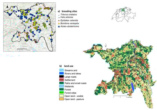
Figure 1.
(a) locations of observed breeding sites from within the last 10 years for each species. In total, there were 12 T. cristatus, 26 H. arborea, 45 E. calamita, 126 B. variegata, and 211 A. obstetricans breeding populations. The figure in the upper right shows the position of the canton of Argau within Switzerland. Basemap source: Esri, HERE, DeLorme, TomTom, Intermap, increment P Corp., GEBCO, USGS, FAO, NPS, NRCAN, GeoBase, IGN, Kadaster NL, Ordnance Survey, Esri Japan, METI, Esri China (Hong Kong), swisstopo, MapmyIndia, © OpenStreetMap contributors, and the GIS User Community; (b) land cover and land use data of the study region (Kanton Aargau) in raster format with a cell size of 10 m2.
2.2. Study Species
Our analysis focused on five amphibian species: the common midwife toad (Alytes obstetricans), the yellow-belied toad (Bombina variegata), the natterjack toad (Epidalea calamita), the European tree frog (Hyla arborea), and the northern crested newt (Triturus cristatus). While the IUCN Red List of Threatened Species designates each species’ conservation status as ‘Least Concern’, all of these species are considered endangered under the most recent edition of Switzerland’s own Red List [28] and are priority species in need of special conservation measures by the Canton Aargau’s Department of Environment [29]. These assessments are the result of widespread population declines and regional disappearances, attributed predominantly to the loss of habitat due to anthropogenic modification of the environment and changes in land use patterns [28].
Like most amphibians, the considered species occupy aquatic and terrestrial habitat alternatively but differ with respect to habitat preferences and movement range. As a result, the distributions and range of habitats occupied by each species both overlap and diverge from each other. For example, E. calamita’s preference of shallow, ephemeral pools contrasts with the deep, cool, and permanent bodies of water where A. obstetricans larvae are typically found. Alternatively, while T. cristatus and B. variegata are often observed in forests, H. arborea and E. calamita normally avoid such terrain. Furthermore, H. arborea and E. calamita are highly mobile species with maximum dispersal ranges of 5 km or greater [30,31], while the three other species rarely move more than a few hundred meters from their natal ponds and have maximum recorded dispersal ranges of 1–2 km [32]. In total, 12 T. cristatus, 26 H. arborea, 45 E. calamita, 126 B. variegata, and 211 A. obstetricans breeding populations were derived from the volunteer-based Amphibian Monitoring Program of Canton Aargau (Figure 1; Table 1). The database contains detailed information for each species within the canton, including the coordinates and estimates of population size for all observed breeding sites dating back to 1992. We included all breeding-pond locations which were occupied at least once during the past 10 years. For ponds with multiple recorded observations, we used the geometric mean of each year’s population size estimate (Table 1). Maximum recorded dispersal distances were assessed using literature findings for each species (Table 1) [30,31,32,33,34].

Table 1.
Amphibian data indicating the number of breeding ponds for each species and the maximum dispersal distances used. Population sizes were classified into four size categories per species.
Due to variations in context and availability of dispersal data, determining a consensus dispersal distance proved challenging for most species. Additionally, citing the strong correlation between dispersal records and study area size, Smith and Green [32] suggest that most dispersal data is likely underestimated as a consequence of mark-recapture study design. As such, with the aim of ensuring the inclusion all possible migration paths in the functional connectivity analyses, we used the maximum values found in the literature for each species and rounded up to the nearest 500 m (Table 1).
2.3. Landscape Map
A raster data set for land use (10 m resolution) was generated for the canton using ArcGIS version 10.2.2 Desktop (Figure 1b; Table A1). Land cover data (polygons) were derived from the Swiss Topological Landscape Model (swissTLM 3D; [35]). Combining this vector data with the 100 m2 resolution GEOSTAT’s Arealstatistik model [36], we refined the category “open land” into intensively (arable land) and extensively used pasture. To avoid border effects in the analysis, the study area was buffered with 5 km. As no land use data was available in the buffer region bordering Germany, the cells were randomly allocated to one of the 10 landscape categories (Figure 1b).
2.4. Landscape Resistance Maps
To account for each amphibian species’ habitat preferences, we generated separate landscape resistance maps for each amphibian species. In the absence of empirical information on landscape resistance for the considered species, two amphibian experts were asked which landscape elements may be considered obstacles and which likely enhance the movement of amphibians (Figure 1b). Experts were asked to rank each land category according to its permeability to movement for each amphibian species. From the resulting lists of rankings, a final master ranking of land cover and land use categories was concatenated for each species (Table 2). By simplifying the rankings into four tiers of resistance (habitat, favorable matrix, less favorable matrix, strong barriers), most differences of opinion between the two experts could be reconciled (Table 3).
Table 2.
Land—land use categories ranked into four tiers according to their resistance to movement for each species, increasing from low (habitat) to high (strong barrier).
Table 3.
Resistance values from each transformation for each landscape resistance tier. Movement habitat and strong barriers were valued at 1 and 1000, respectively. The dotted lines indicate the locations of high contrast transitions between resistance tiers.
Using these rankings, we calculated cost maps based on a suite of resistance-value transformations: null, exponential, sigmoidal, logarithmic, and linear (Figure 2). Each set of values was scaled from 1 to 1000 (no resistance (habitat) = 1, high resistance (strong barriers) = 1000). With reasonable success, the exponential power of 10 sequence has been commonly used in the literature to assign increasing resistance values to gradients of poorer habitat when empirical movement data are unavailable [24,37]. Alternatively, Rayfield and Fortin [38] showed that least-cost analysis results are most sensitive to the location of high contrast transitions between the values of resistance categories. To account for this, we chose to complement the exponential resistance scale with the sigmoidal, logarithmic, and linear scenarios (Figure 2, Table 3). Additionally, a null model was chosen that only penalized movement through strong barriers, considering all other land cover and land use categories equally permeable (Figure 2).
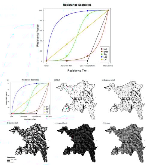
Figure 2.
(a) the five theoretical resistance scenario transformations used to create the resistance maps; (b–f) show examples of the five resistance maps used in Circuitscape analyses for each species (seen here for A. obstetricans). Cells are shaded from white to black with increasing resistance. Each resistance map is derived by assigning one of the five resistance. scenarios from panel (a) to the habitat resistance rankings for each species in Table 1.
2.5. Modelling Connectivity
Circuitscape [25] is an open-source program based off of linkages between circuit and random walk theories that models the connectivity of a species in its surrounding landscape by relating dispersal to electricity moving along a circuit board [25]. A landscape is described by a resistance map, a grid of raster cells which represent the permeability of habitat to movement for a given species in the study landscape. Current density maps produced by connecting current between pairs of populations across the resistance map display the probability that a random walker would move through each pixel in a landscape. The model has been widely used by ecologists for its powerful ability to generate predictions of movement patterns for a broad range of species at both small and large scales [27,37,39,40]. The landscape is described as a resistance map, a grid of raster cells which represent the varying qualities of habitat or movement barriers tailored to a given species in the landscape. Source and ground nodes representing start- and end-points for movements are then connected, producing a current map that illustrates the probability of species movement through each cell of the landscape. As an advantage over least-cost analyses, potentially all movement routes are considered simultaneously, generating a continuous map of probabilities across the entire study region [41]. Circuitscape has been commonly used to model functional connectivity following one of two approaches that both produce valid yet different results. The first approach relies on species distribution data to place the source and ground nodes through which current is connected in order to predict movement patterns between occupied habitat patches [27,40,41]. By weighting current according to population size or habitat quality, abundance data can also be fit into the model. Likewise, node pair exclusions allow the introduction of species dispersal limitations. The resulting current maps estimate the realized functional connectivity occurring within the species’ distribution as it exists today. Alternatively, a number of studies forego the inclusion of independently collected species data (which can be cost- and time-consuming to generate), instead placing nodes along the perimeter of a buffered study landscape [37,42,43]. The result is a continuous current map that is unbiased by the placement of nodes or sensitive to variation in empirical data. These maps describe the potential functional connectivity of the landscape, or species-specific structural connectivity, highlighting movement paths across the entire region, even in areas where the species is absent.
We used Circuitscape (version 4.0.5) to model two different interpretations of landscape connectivity for each amphibian species in Aargau [25]. The first set of models made use of available population data from the Amphibian Monitoring Program to estimate the functional connectivity that exists between the distributions of each species as they exist today. These maps indicate the relative likelihood of movement occurring across all cells in the landscape for each species under the five different resistance scenarios. Circuitscape was run in pairwise mode, using the amphibian breeding sites (Figure 1) as the source and ground nodes for current, iteratively connecting all possible pairings. If the distance between ponds exceeded the maximum dispersal distance of a given species (Table 1), that pairing was excluded from the analysis. To reduce processing times, all regions of the resistance maps that were outside of the maximum dispersal range of any breeding pond were masked out. Following the hypothesis that the number of emigrants from a subpopulation scales with population size, the current leaving each breeding pond was varied according to its geometric mean population size between 2006 and 2016. As the option to vary source node strength in pairwise mode does not (yet) exist in Circuitscape, each pairwise map was multiplied by the geometric means of the included populations. By adding each weighted pairwise map, a cumulative current density map was generated for each species and resistance scenario, highlighting the relative likelihood of movement occurring between subpopulations as they are presently situated in the region.
From the individual species current maps, a final multi-species cumulative-current map was calculated for the exponential resistance scenario. Absolute current values in the functional connectivity maps scaled differently among species due to large differences in the number and size of subpopulations. Therefore, we first normalized each species current map on a scale between 0 and 1 before summing them together in order to ensure equal representation of all species in the multi-species functional current maps.
A second set of models was generated which assessed species-specific structural connectivity across the entire study region. We ignored the present distributions and dispersal limitations of each species, instead connecting current between randomly placed nodes along the perimeter of the study region. Based entirely upon each species’ resistance map, these maps describe the landscape’s potential for connectivity for a given species. Like the multi-species functional connectivity map, each species map was normalized before combining into multi-species structural connectivity maps. The functional and structural multi-species connectivity maps highlight important regions shared by all species.
2.6. Sensitivity Analysis
To examine the degree to which the selection of resistance values impacts the resulting current maps, we measured the percent overlap of the locations of high current regions and calculated Spearman’s rank correlations between each resistance scenario. To calculate the percent overlap among resistance sets, we compared the locations of cells with the highest 20% current values after omitting all cells with a current of zero. Since it was expected that each current map would have a current density bias in the cells immediately surrounding each breeding site, we dropped the top 5% of cells in order to focus on overlap occurring away from the source and ground nodes. Alternatively, correlation was calculated using Spearman’s rank coefficient as the absolute current values in each cell scaled differently depending on the transformation of resistance values. We randomly selected 5% of the cells from the masked study regions used in the Circuitscape analyses and compared current values between each resistance set. From the results of both metrics, we then calculated the mean and standard deviation for each pairwise comparison across species.
3. Results
3.1. Connectivity Analysis
Each species’ cumulative current map generated using population data displays an overview of areas where functional connectivity among breeding populations is high (Figure 3a; see Figure A1 for all individual species). High current regions signify areas with an increased relative likelihood of movement occurring in each cell as a function of population size, the density of interconnected breeding sites, and the degree to which the landscape restricts and concentrates movement. The multispecies functional connectivity current map (Figure 3a) identifies regions with overlapping corridors of high movement potential, most notably along the river Reuss in the east of the canton, the only region where all five species are present. Additional high current locations include the northeastern region near Zurzach and the central region along the Aare, where the midwife, yellow-bellied, and natterjack toads all exhibit relatively high functional connectivity (Figure A1).
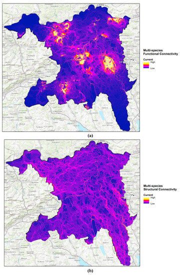
Figure 3.
(a) multispecies functional and (b) structural connectivity maps under the exponential resistance scenario. The discrete color scale, from dark blue (0) to yellow (5), indicates the number of species for which each cell has a high connectivity current value.
The multi-species structural connectivity maps (Figure 3b; see Figure A2 for individual species) highlight where connectivity is collectively high among species based on structural information. It is evident that there are no large swaths of land which all species are likely to find permeable. The majority of high current cells are streams and ponds, but there also exist small tracts of land where the movements of all species are concentrated into important habitat connections. While functional connectivity as expressed as breeding-population size and actual movement distance shows rather well-defined hotspots of connectivity, the connectivity map based on structural information results in decentralized movement paths with spatially distributed and unspecific movement pathways.
3.2. Resistance Scenarios
The percentage of overlap in the locations of high current cells among pairwise comparisons of resistance scenarios ranged from 41–90% (Table 4). All comparisons to the null resistance scenario had notably less overlap in all species (41–50% vs. 60–90%), indicating the strong effect that the inclusion of matrix landscape categories has on the current maps. Spearman’s rank correlation coefficients were distinctly lower, varying from 0.15–0.56 (Table 5). Once again, comparisons to the null resistance scenario had the least agreement (0.15–0.27 vs. 0.34–0.56). Excluding the null scenario, the exponential resistance scenario was predictably in lowest agreement with its inverse, the logarithmic, and, to a lesser degree, the linear model for both metrics. These two scenarios both assign very high resistance values to the matrix categories compared to the exponential as can be seen in Figure 3. However, it is interesting that, despite this strong contrast, comparisons between these scenarios are still favored over the null scenario. Even a slight structuring of the landscape into habitat/matrix classes evidently leads to a reasonably similar configuration of high current regions in the map. Alternatively, across species, standard deviations are notably different between the two metrics. While quite low in the overlap analysis, variation among species in the correlation analysis was uniformly high. Species differences could be due to a multitude of factors, many of which would be derived by the interactive effects between species-specific resistance rankings and the differences in the landscape included in each species’ own masked study region (configuration, fragmentation, and composition). However, fundamentally, this variation shows the high sensitivity each species’ current map exhibits to the choice of resistance scenario at a finer scale, where relative current values among cells are considered.
Table 4.
Sensitivity analysis results comparing the functional connectivity current maps generated under each resistance scenario. Across species means and standard deviations for the pairwise comparisons of the percentage of overlapping high current cells. Percent overlap was calculated by comparing the locations of cells with the highest 20% current, after excluding the highest 5%.
Table 5.
Sensitivity analysis results comparing the functional connectivity current maps generated under each resistance scenario. Across species means and standard deviations for the pairwise comparisons of Spearman’s rank correlation coefficient between cells of each current map. Correlation coefficients were calculated by randomly selecting 5% of the cells in the masked study region of each species.
4. Discussion
Recently, claims to include connectivity assessments into green infrastructure concepts have been put forward as they may provide important baseline information to preserve and mitigate threats of habitat fragmentation [9]. Here, we provided a regional-scale multispecies connectivity map to analyze the movement potential of amphibian species across a human-dominated landscape. The multispecies approach accounts for each species’ estimated or known dispersal ability and modulates the dispersal (“current”) strength based on the population size, thus allowing for a spatial source-sink dynamic. The results from this functional connectivity assessment are contrasted by an analysis relying solely on expert-based judgement on the potential connectivity given landscape structure only. The complementary aspects of the functional and structural connectivity maps provide a picture of realized and potential connectivity, together offering the insight required to preserve and mitigate threats to connectivity or improve and restore it. The sensitivity analysis showed that each species’ current map is highly sensitive to the choice of resistance scenarios.
There are various multispecies approaches in connectivity assessments, for example selecting ‘umbrella species’, assuming that a broad range of associated species would benefit from measures taken to preserve or restore connectivity for a particular species [44,45,46]. However, identifying suitable surrogate species has remained a debated challenge [47,48,49]. Alternatively, Koen et al. [37] produced a regional map of potential functional connectivity for a generalized suite of forest-dwelling species that successfully predicted the movement corridors of a bird and several amphibian species. However, this approach lacks flexibility, as it is limited to groups of species that share a similar behavioral response to the landscape patterns. When the permeability of the landscape differs substantially among the focal species of a study, it would seem necessary to include separate resistance surfaces tailored to each species within the analysis. Beier et al. [47] achieved this by overlaying the movement corridors predicted by individual species models in a multi-species least-cost path analysis of connectivity. Using Circuitscape [25,26], however, insights are not limited to a few specific habitat patches or corridors, but are available in continuous, high-resolution, and large-scale maps across the study region indicating all potential movement routes. The species-specific approach used to generate the multispecies current maps offers the flexibility to include species with diverse movement ecologies and ensures that no species is potentially mismatched to the requirements of a single ‘umbrella’ species. The target species included in the analysis could even be expanded to include other groups of species, e.g., dragonflies or other wetland species that could synergistically benefit from conservation initiatives. While the multispecies current maps provide insights that can be used to improve landscape connectivity for some or all of these species, each individual species current map can also be used independently to prioritize regions of focus in conservation efforts and in the identification of integral landscape features to connectivity for a single target species.
However, lacking independent movement data to validate the connectivity models and the resistance maps they are derived from, it is difficult to assess just how accurate these maps are. Despite reasonably high overlap of high current regions in the sensitivity analysis, the breadth of landscape resistance scenarios captured by the analysis is by no means all-inclusive. It is also not likely that landscape categories can be discretely divided into categories of resistance rankings, or that the number of categories would be equal across species. In addition, only land cover/land use was considered. Other factors, such as pollution and habitat quality, weather conditions, traffic volumes, or microhabitats may additionally impact movement patterns of amphibians [31,50].
Therefore, options to improve connectivity models are manifold. It is well established that connectivity analyses based on expert knowledge generally perform worse than and are best applied only as a complement to more data-driven approaches [11,17]. Empirically derived field-data that accurately relates the movement of dispersers to the landscape would improve the spatial aspects of dispersal [12]. There are a number of methods available to landscape ecologists for this purpose. Mark-recapture and telemetry studies can quantify the movement rates, distances, and paths of individuals in order to identify the behavioral responses of a species to its environment. Besides being quite resource-intensive, the challenge with these methods is capturing the movements of an actual disperser. Many amphibians have a high fidelity to their natal ponds, and dispersal rates between breeding populations can be very low [51]. Movement patterns of an amphibian within its terrestrial home range likely differ to that of a dispersing individual exposed to various qualities of matrix habitat over much greater distances [50,52]. Alternatively, the use of gene flow as a measure to delineate connectivity among populations has been widely applied [53,54,55], also in a conservation context [56,57]. Through the comparison of the genetic characteristics between breeding ponds, it is possible generate estimates of gene flow that can then be used to estimate the resistance values of landscape features that separate them after accounting for the multigenerational processes that determine genetic structures [1].
It is also important to note that the current maps only indirectly describe the actual quality of the landscape with respect to supporting connectivity. High current regions within the functional connectivity maps are predominantly determined by the size and number of connected breeding populations; landscape resistance simply shapes the flow of current. Generally, current that flows across regions of poor permeability to movement will be highly concentrated through the few landscape features that promote movement, like streams. Alternatively, in areas where the terrain is broadly favourable to movement, current flow unrestricted in wider swaths. Furthermore, if absolutely no movement corridors exist through poor terrain, the flow of current will be indistinguishable from that of a uniformly high quality region of connectivity. Distinguishing such scenarios from these current maps requires a keen eye and familiarity with the terrain. Sinsch’s et al. [58] review of the literature suggests that this may actually be an accurate portrayal of the effect of landscape resistance on amphibian movements. However, it is also likely that the high cost of dispersal over a poorer matrix habitat has a negative effect on the likelihood of an immigrant’s reproduction success, which should be factored into predictions of functional connectivity [1]. Circuitscape calculates an ‘effective resistance’ metric between each node pair as a function of the cumulative cost-distance and redundancy of paths between nodes [26]. Further weighting of the amount of current flow between nodes by effective resistance may allow a better representation of functional connectivity within the region that takes into account landscape quality.
5. Conclusions
Regardless of the limitations of the models within this study, we believe that the methods outlined here to generate functional and species-specific structural connectivity maps could be very valuable to conservation efforts for these species and, if scaled up accordingly, for even more species and regions. Both sets of current maps, functional and structural, provide a great deal of information concerning landscape connectivity and could seemingly be used in a multitude of conservation-related applications. The functional connectivity current maps act as excellent visual aids that are easily accessible and intuitively allow a user to locate areas within each species’ distribution where connectivity is high or low on a cantonal scale. Focusing in on specific areas elucidates the importance of fine-scale features that can inform decisions in development and land use change, suggest locations along highways where amphibian tunnels may be needed, or identify sensitive movement corridors that could benefit from reinforcing protective measures. The structural connectivity maps can guide restoration efforts, highlighting suitable locations for the creation of stepping stone ponds between isolated clusters of breeding populations. In addition, such maps could provide decision-makers with the insight needed to mitigate the impact of development on biodiversity and identify regions where landscape connectivity can be improved. This feature is particularly relevant in the context of designing green infrastructure [9], a concept in spatial planning policy included in the EU2020 Biodiversity Strategy that involves the strategic planning of development and land use to ensure the long-term persistence of biodiversity and ecosystem services [9,59,60,61]; EEA (https://www.eea.europa.eu/themes/sustainability-transitions/urban-environment/urban-green-infrastructure/what-is-green-infrastructure).
Additionally, approaches to overcome the computer-intensive analysis with Circuitscape may allow large scale maps [23,43], allowing for large-scale multi-species connectivity maps capable of guiding the needs of conservation efforts.
Author Contributions
Gregory Churko: conceptualization, visualization, writing—original draft preparation, and writing—review. Felix Kienast: conceptualization and writing—original draft preparation. Janine Bolliger: conceptualization, writing—original draft preparation, and writing—review. All authors have read and agreed to the published version of the manuscript.
Funding
This research received no external funding.
Acknowledgments
We thank Benedikt Schmidt (karch) and Christoph Bühler (Hintermann and Weber) for their input for calibrating the species resistance maps.
Conflicts of Interest
The authors declare no conflict of interest.
Appendix A. Generating the Landscape Model
Table A1.
m (one cell width) except for fine-scale linear features like streams and paths (5 m), or the low drawing order / low resolution land use categories (none). Major roads were buffered by 15 m to ensure that they were always drawn at least two cells wide and acted as strong barriers (current jumps easily across the curves of linear single cell barriers in raster datasets because barrier cells are only connected at the corners instead of their sides). Any cell within the map lacking classification after filling the model with all other categories was assigned to ‘Pasture’. This was done under the assumption that most of these cells would be marginal, undeveloped, open vegetated land, such as the areas around highway approaches, which would have similar characteristics to pastures.
| Drawing Order | Land Cover/Land Use | Source | Selection | Type | Buffer | Notes |
|---|---|---|---|---|---|---|
| 1 | Streams Ponds Lake and river margins | TLM_FLIESSGEWAESSER_2015 TLM_BODENBEDECKUNG_2015 TLM_BODENBEDECKUNG_2015 | Objektart = Fliessgewaesser (4) + Verlauf = Oberirdisch (100) Objektart = Stehende Gewaesser (10) + ShapeArea < 600,000 Objektart = Fliessgewaesser (5) + ShapeArea/ShapeLength > 10 Objektart = Stehende Gewaesser (10) + ShapeArea > 600,000 | Polyline Polygon Polygon | 5 m full 10 m full −10 m outside_only | There is an overlap between the two data sources for streams and rivers => all stream polylines that intersected river polygons were considered rivers |
| 2 | Rivers and lakes | TLM_BODENBEDECKUNG_2015 | Objektart = Fliessgewaesser (5) + ShapeArea/ShapeLength > 10 Objektart = Stehende Gewaesser (10) + ShapeArea > 600,000 | Polygon | None | Wetlands and lakes overlap in some locations => these were erased from the lake polygons |
| 3 | Major roads | TLM_STRASSE_2015 | Objektart = Autobahn, Autostrassen, 6 m, 8 m, 10m Strasse (2, 21, 9, 20, 8) | Polyline | 15 m full | |
| 4 | Settlements | TLM_GEBAUDE_FOOTPRINT_2015 | Objektart = Gebaude, etc (1-5) | Polygon | 10 m full | Overlapping features dissolved together |
| 5 | Paths and minor roads | TLM_STRASSE_2015 | Objektart = 3m Strasse, 2 m Wed (11,15) | Polyline | 5 m full | |
| 6 | Wetlands | TLM_BODENBEDECKUNG_2015 | Objektart = Feuchtgebiet (11) | Polygon | 10 m full | |
| 7 | Forest | TLM_BODENBEDECKUNG_2015 | Objektart = Wald, Wald offen (12, 13) | Polygon | None | |
| 8 | Forest margin | TLM_BODENBEDECKUNG_2015 | Objektart = Wald, Wald offen (12, 13) | Polygon | −10 m outside only | |
| 9 | Arable land | Areal Statistik 2004/2009 | Objektart = Ackerland (41) | Raster (100 m cell size) | None | 100 m raster cells resampled down to 10 m |
| 10 | Pasture | Areal Statistik 2004/2009 | Objektart = Naturwiesen (42) and Heimwieden (43), + No Data | Raster (100 m cell size) | None | 100 m raster cells resampled down to 10 m |

Figure A1.
Functional connectivity maps for Bombina variegata, Triturus cristatus, Epidalea calamita, Hyla arborea, and Alytes obstetricans. The green circles indicate the locations of breeding sites.

Figure A2.
Structural connectivity maps for Bombina variegata, Triturus cristatus, Epidalea calamita, Hyla arborea, and Alytes obstetricans.
References
- Baguette, M.; Blanchet, S.; Legrand, D.; Stevens, V.M.; Turlure, C. Individual dispersal, landscape connectivity and ecological networks. Biol. Rev. 2013, 88, 310–326. [Google Scholar] [CrossRef] [PubMed]
- Cayuela, H.; Lambrey, J.; Vacher, J.P.; Miaud, C. Highlighting the effecs of land-use change on a threatened amphibian in a human-dominated landscape. Popul. Ecol. 2015, 57, 433–443. [Google Scholar] [CrossRef]
- Eterovick, P.C.; Sloss, B.L.; Scalzo, J.A.M.; Alford, R.A. Isolated frogs in a crowded world: Effects of human-caused habitat loss on frog heterozygosity and fluctuating asymmetry. Biol. Conserv. 2016, 195, 52–59. [Google Scholar] [CrossRef]
- Bowne, D.R.; Bowers, M.A. Interpatch movements in spatially structured populations: A literature review. Landsc. Ecol. 2004, 19, 1–20. [Google Scholar] [CrossRef]
- Fahrig, L. Effect of habitat fragmentation on the extinction threshold: A synthesis. Ecol. Appl. 2002, 12, 346–353. [Google Scholar]
- Allen, C.; Gonzales, R.; Parrott, L. Modelling the contribution of ephemeral wetlands to landscape connectivity. Ecol. Model. 2020, 419. [Google Scholar] [CrossRef]
- Stuart, S.N.; Chanson, J.S.; Cox, N.A.; Young, B.E.; Rodrigues, A.S.L.; Fischman, D.L.; Waller, R.W. Status and trends of amphibian declines and extinctinos worldwide. Science 2004, 306, 183–186. [Google Scholar] [CrossRef]
- Cushman, S.A.; Shirk, A.J.; Landguth, E.L. Landscape genetics and limiting factors. Conserv. Genet. 2013, 14, 263–274. [Google Scholar] [CrossRef]
- Bolliger, J.; Silbernagel, J. Contribution of connectivity assessments to Green Infrastructure (GI). ISPRS Int. J. Geo Inf. 2020, 9, 212. [Google Scholar] [CrossRef]
- Naidoo, R.; Kilian, J.W.; Du Preez, P.; Beytell, P.; Aschenborn, O.; Taylor, R.D.; Stuart-Hill, G. Evaluating the effectiveness of local- and regional-scale wildlife corridors using quantitative metrics of functional connectivity. Biol. Conserv. 2018, 217, 96–103. [Google Scholar] [CrossRef]
- Milanesi, P.; Holderegger, R.; Caniglia, R.; Fabbri, E.; Galaverni, M.; Randi, E. Expert-based versus habitat-suitability models to develop resistance surfaces in landscape genetics. Oecologia 2017, 183, 67–79. [Google Scholar] [CrossRef] [PubMed]
- Zeller, K.A.; Jennings, M.K.; Vickers, T.W.; Ernest, H.B.; Cushman, S.A.; Boyce, W.M. Are all data types and connectivity models created equal? Validating common connectivity approaches with dispersal data. Divers. Distrib. 2018, 24, 868–879. [Google Scholar] [CrossRef]
- Parks, L.C.; Wallin, D.O.; Cushman, S.A.; McRae, B.H. Landscape-level analysis of mountain goat population connectivity in Washington and southern British Columbia. Conserv. Genet. 2015, 16, 1195–1207. [Google Scholar] [CrossRef]
- Squires, J.R.; DeCesare, N.J.; Olson, L.E.; Kolbe, J.A.; Hebblewhite, M.; Parks, S.A. Combining resource selection and movement behavior to predict corridors for Canada lynx at their southern range periphery. Biol. Conserv. 2013, 157, 187–195. [Google Scholar] [CrossRef]
- Wasserman, T.N.; Cushman, S.A.; Schwartz, M.K.; Wallin, D.O. Spatial scaling and multi-model inference in landscape genetics: Martes americana in northern Idaho. Landsc. Ecol. 2010, 25, 1601–1612. [Google Scholar] [CrossRef]
- Fattebert, J.; Robinson, H.S.; Balme, G.; Slotow, R.; Hunter, L. Structural habitat predicts functional dispersal habitat of a large carnivore: How leopards change spots. Ecol. Appl. 2015, 25, 1911–1921. [Google Scholar] [CrossRef]
- Reed, G.C.; Litvaitis, J.A.; Callahan, C.; Carroll, R.P.; Litvaitis, M.K.; Broman, D.J.A. Modeling landscape connectivity for bobcats using expert-opinion and empirically derived models: How well do they work? Anim. Conserv. 2017, 20, 308–320. [Google Scholar] [CrossRef]
- Marrotte, R.R.; Bowman, J.; Brown, M.G.C.; Cordes, C.; Morris, K.Y.; Prentice, M.B.; Wilson, P.J. Multi-species genetic connectivity in a terrestrial habitat network. Mov. Ecol. 2017, 5, 21. [Google Scholar] [CrossRef]
- Fleishman, E.; Anderson, J.; Dickson, B.G. Single-species and multiple-species connectivity models for large mammals on the Navajo nation. West. N. Am. Nat. 2017, 77, 237–251. [Google Scholar] [CrossRef]
- Bleyhl, B.; Baumann, M.; Griffiths, P.; Heidelberg, A.; Manvelyan, K.; Radeloff, V.C.; Zazanashvili, N.; Kuemmerle, T. Assessing landscape connectivity for large mammals in the Caucasus using Landsat 8 seasonal image composites. Remote Sens. Environ. 2017, 193, 193–203. [Google Scholar] [CrossRef]
- Brodie, J.F.; Giordano, A.J.; Dickson, B.G.; Hebblewhite, M.; Bernard, H.; Mohd-Azlan, J.; Anderson, J.; Ambu, L. Evaluating multispecies landscape connectivity in a threatened tropical mammal community. Conserv. Biol. 2015, 29, 122–132. [Google Scholar] [CrossRef] [PubMed]
- Keller, D.; Holderegger, R.; Van Strien, M.J.; Bolliger, J. How to make landscape genetics beneficial for conservation management? Conserv. Genet. 2015, 16, 503–512. [Google Scholar] [CrossRef]
- Koen, E.L.; Ellington, E.H.; Bowman, J. Mapping landscape connectivity for large spatial extents. Landsc. Ecol. 2019, 34, 2421–2433. [Google Scholar] [CrossRef]
- Clauzel, C.; Bannwarth, C.; Foltete, J.C. Integrating regional-scale connectivity in habitat restoration: An application for amphibian conservation in eastern France. J. Nat. Conserv. 2015, 23, 98–107. [Google Scholar] [CrossRef]
- McRae, B.H.; Dickson, B.G.; Keitt, T.H.; Shah, V.B. Using circuit theory to model connectivity in ecology and conservation. Ecology 2008, 10, 2712–2724. [Google Scholar] [CrossRef]
- McRae, B.H.; Beier, P. Circuit theory predicts gene flow in plant and animal populations. Proc. Natl. Acad. Sci. USA 2007, 104, 19885–19890. [Google Scholar] [CrossRef]
- Dickson, B.G.; Albano, C.M.; Anantharaman, R.; Beier, P.; Fargione, J.; Graves, T.A.; Gray, M.E.; Hall, K.R.; Lawler, J.J.; Leonard, P.B.; et al. Circuit-theory applications to connectivity science and conservation. Conserv. Biol. 2019, 33, 239–249. [Google Scholar] [CrossRef]
- Schmidt, B.R.; Zumbach, S. Rote Liste der Gefährdeten Amphibien der Schweiz, 1st ed.; Bundesamt für Umwelt, Wald und Landschaft (BUWAL); Koordinationsstelle für Amphibien- und Reptilienschutz in der Schweiz (KARCH): Bern, Switzerland, 2005; p. 48. [Google Scholar]
- Meier, C.; Schelbert, B. Amphibienschutzkonzept Kanton Aargau. Mitt. Aargauer Nat. Ges. 1999, 35, 41–69. [Google Scholar]
- Le Lay, G.; Angelone, S.; Flory, C.; Holderegger, R.; Bolliger, J. Increasing pond density to maintain a patchy habitat network of the European tree frog (Hyla arborea). J. Herpetol. 2015, 49, 217–221. [Google Scholar] [CrossRef]
- Frei, M.; Csencsics, C.; Brodbeck, S.; Schweizer, E.; Bühler, C.; Gugerli, F.; Bolliger, J. Combining landscape genetics, radio-tracking and long-term monitoring to derive management implications for Natterjack toads (Epidalea calamita) in agricultural landscapes. J. Nat. Conserv. 2016, 32, 22–34. [Google Scholar] [CrossRef]
- Smith, M.A.; Green, D.M. Dispersal and the metapopulation paradigm in amphibian ecology and conservation: Are all amphibian populations metapopulations? Ecography 2005, 28, 110–128. [Google Scholar] [CrossRef]
- Primus, J. Disperal and Migration in Yellow-Bellied Toads, Bombina Variegata; University of Vienna: Vienna, Austria, 2013. [Google Scholar]
- Baker, J.; Beebee, T.; Buckley, J.; Gent, A.; Orchard, D. Amphibian Habitat Management Handbook; Amphibian and Reptile Conservation: Bournemouth, UK, 2011. [Google Scholar]
- swissTLM 3D. Vectorized National Map 1:25’000, Bundesamt für Landestopographie; Swisstopo: Wabern, Switzerland, 2015. [Google Scholar]
- BfS, S. Land Use in Switzerland: Results of the Swiss Land Use Statistics; Federal Statistical Office: Neuchatel, Switzerland, 2013.
- Koen, E.L.; Bowman, J.; Sadowski, C.; Walpole, A.A. Landscape connectivity for wildlife: Development and validation of multispecies linkage maps. Methods Ecol. Evol. 2014, 5, 626–633. [Google Scholar] [CrossRef]
- Rayfield, B.; Fortin, M.J.; Fall, A. The sensitivity of least-cost habitat graphs to relative cost surface values. Landsc. Ecol. 2010, 25, 519–532. [Google Scholar] [CrossRef]
- Braaker, S.; Moretti, M.; Boesch, R.; Ghazoul, J.; Obrist, M.K.; Bontadina, F. Assessing habitat connectivity for ground-dwelling animals in an urban environment. Ecol. Appl. 2014, 24, 1583–1595. [Google Scholar] [CrossRef] [PubMed]
- Nowakowski, A.J.; Veiman-Echeverria, M.; Kurz, D.J.; Donnelly, M.A. Evaluating connectivity for tropical amphibians using empirically derived resistance surfaces. Ecol. Appl. 2015, 25, 928–942. [Google Scholar] [CrossRef]
- McRae, B.H.; Schumaker, N.; McKane, R.; Busing, R.; Solomon, A.; Burdick, C. A multi-model framework for simulating wildlife population response to land use and climate change. Ecol. Model. 2008, 219, 77–79. [Google Scholar] [CrossRef]
- Walpole, A.A.; Bowman, J.; Murray, D.L.; Wilson, P.J. Functional connectivity of lynx at their southern range periphery in Ontario, Canada. Landsc. Ecol. 2012, 27, 761–773. [Google Scholar] [CrossRef]
- Pelletier, D.; Clark, M.; Anderson, M.G.; Rayfield, B.; Wulder, M.A.; Cardille, J.A. Applying Circuit Theory for Corridor Expansion and Management at Regional Scales: Tiling, Pinch Points, and Omnidirectional Connectivity. PLoS ONE 2014, 9. [Google Scholar] [CrossRef]
- Beier, C.M. Influence of Political Opposition and Compromise on Conservation Outcomes in the Tongass National Forest, Alaska. Conserv. Biol. 2008, 22, 1485–1496. [Google Scholar] [CrossRef]
- Breckheimer, I.; Haddad, N.M.; Morris, W.F.; Trainor, A.M.; Fields, W.R.; Jobe, R.T.; Hudgens, B.R.; Moody, A.; Walters, J.R. Defining and evaluating the umbrella species concept for conserving and restoring landscape connectivity. Conserv. Biol. 2014, 28, 1584–1593. [Google Scholar] [CrossRef]
- Mikolas, M.; Tejkal, M.; Kuemmerle, T.; Griffiths, P.; Svoboda, M.; Hlasny, T.; Leitao, P.J.; Morrissey, R.C. Forest management impacts on capercaillie (Tetrao urogallus) habitat distribution and connectivity in the Carpathians. Landsc. Ecol. 2017, 32, 163–179. [Google Scholar] [CrossRef]
- Beier, P.; Majka, D.R.; Newell, S.L. Uncertainty analysis of least-cost modeling for designing wildlife linkages. Ecol. Appl. 2009, 19, 2067–2077. [Google Scholar] [CrossRef] [PubMed]
- Dondina, O.; Orioli, V.; Chiatante, G.; Bani, L. Practical insights to select focal species and design priority areas for conservation. Ecol. Indic. 2020, 108. [Google Scholar] [CrossRef]
- Meurant, M.; Gonzalez, A.; Doxa, A.; Albert, C.H. Selecting surrogate species for connectivity conservation. Biol. Conserv. 2018, 227, 326–334. [Google Scholar] [CrossRef]
- Peterman, W.E.; Connette, G.M.; Semlitsch, R.D.; Eggert, L.S. Ecological resistance surfaces predict fine-scale genetic differentiation in a terrestrial woodland salamander. Mol. Ecol. 2014, 23, 2402–2413. [Google Scholar] [CrossRef] [PubMed]
- Frei, M.; Csencsics, D.; Bühler, C.; Gugerli, F.; Bolliger, J. Wie gut vernetzt sind Vorkommen der Kreuzkröte in einer landwirtschaftlich geprägten Landschaft? N. L. Inside 2014, 4, 16–20. [Google Scholar]
- Abrahms, B.; DiPietro, D.; Graffis, A.; Hollander, A. Managing biodiversity under climate change: Challenges, frameworks, and tools for adaptation. Biodivers. Conserv. 2017, 26, 2277–2293. [Google Scholar] [CrossRef]
- Bolliger, J.; Keller, D.; Holderegger, R. When landscape variables do not explain migration rates: An example from an endangered dragonfly (Leucorrhinia caudalis). Eur. J. Entomol. 2011, 108, 327–330. [Google Scholar] [CrossRef]
- Keller, D.; Van Strien, M.J.; Ghazoul, J.; Holderegger, R. Landscape Genetics of Insects in Intensive Agriculture: New Ecological Insights; Swiss Federal Research Institute WSL: Birmensdorf, Switzerland, 2012.
- Keller, D.; Van Strien, M.J.; Holderegger, R. Do landscape barriers affect functional connectivity of populations of an endangered damselfly? Freshw. Biol. 2012, 57, 1373–1384. [Google Scholar] [CrossRef]
- Bolliger, J.; Lander, T.; Balkenhol, N. Landscape genetics since 2003: Status, challenges and future directions. Landsc. Ecol. 2014, 29, 361–366. [Google Scholar] [CrossRef]
- Holderegger, R.; Balkenhol, N.; Bolliger, J.; Engler, J.O.; Gugerli, F.; Hochkirch, A.; Nowak, C.; Segelbacher, G.; Widmer, A.; Zachos, F.E. Conservation genetics: Linking science with practice. Mol. Ecol. 2019, 28, 3848–3856. [Google Scholar] [CrossRef] [PubMed]
- Sinsch, U.; Oromi, N.; Miaud, C.; Denton, J.; Sanuy, D. Connectivity of local amphibian populations: Modelling the migratory capacity of radio-tracked Natterjack toads. Anim. Conserv. 2012, 15, 388–396. [Google Scholar] [CrossRef]
- Wang, J.X.; Banzhaf, E. Towards a better understanding of Green Infrastructure: A critical review. Ecol. Indic. 2018, 85, 758–772. [Google Scholar] [CrossRef]
- Snäll, T.; Lehtomäki, J.; Arponen, A.; Elith, J.; Moilanen, A. Green infrastructure design based on spatial conservation prioritization and modeling of biodiversity features and ecosystem services. Environ. Manag. 2016, 57, 251–256. [Google Scholar]
- European Commission. Green Infrastructure (GI)—Enhancing Europe’s Natural Capital; European Commission: Brussels, Belgium, 2013; p. 149. [Google Scholar]
© 2020 by the authors. Licensee MDPI, Basel, Switzerland. This article is an open access article distributed under the terms and conditions of the Creative Commons Attribution (CC BY) license (http://creativecommons.org/licenses/by/4.0/).