Abstract
Singular value decomposition (SVD) is ubiquitously used in recommendation systems to estimate and predict values based on latent features obtained through matrix factorization. But, oblivious of location information, SVD has limitations in predicting variables that have strong spatial autocorrelation, such as housing prices which strongly depend on spatial properties such as the neighborhood and school districts. In this work, we build an algorithm that integrates the latent feature learning capabilities of truncated SVD with kriging, which is called SVD-Regression Kriging (SVD-RK). In doing so, we address the problem of modeling and predicting spatially autocorrelated data for recommender engines using real estate housing prices by integrating spatial statistics. We also show that SVD-RK outperforms purely latent features based solutions as well as purely spatial approaches like Geographically Weighted Regression (GWR). Our proposed algorithm, SVD-RK, integrates the results of truncated SVD as an independent variable into a regression kriging approach. We show experimentally, that latent house price patterns learned using SVD are able to improve house price predictions of ordinary kriging in areas where house prices fluctuate locally. For areas where house prices are strongly spatially autocorrelated, evident by a house pricing variogram showing that the data can be mostly explained by spatial information only, we propose to feed the results of SVD into a geographically weighted regression model to outperform the orginary kriging approach.
1. Introduction
The price of a house or apartment is challenging to estimate. The price not only depends on various variables of the house itself, such as the number of rooms, but also on the location [1]. Different school districts [2], proximity to public transport [3], and safety of the neighborhood [4] affect the price of a house. Fluctuations in house prices can have a strong impact on real economic activity. For instance, the rapid rise and subsequent collapse in US residential housing prices is widely considered as one of the major causalities of the financial crisis of 2007–2009 [5], which has in turn led to a deep recession and a protracted decline in employment. In this work, our goal is to leverage powerful, but spatially oblivious, recommendation systems to improve geostatistics for house price estimation.
Recommender engines have become an integral part of our e-commerce. With the progression of the recommender systems, there have been many improvements to it’s implementation. Recommender system engines allow to predict the price of a house by leveraging knowledge about similar houses and their prices. One enhancement has been in integrating spatial elements [6,7] based on Tobler’s first law of geography. The idea of these existing work is to build individial recommender systems for each areal unit.
In this work, in addition to building a recommender system for each region, we feed the results of recommender systems, namely using matrix factorization, directly into a geostatistical interpolation, namely regression kriging. Combined, our approach leverages the strong predictive power of matrix factorization by building successive latent variables explaining most of the inter-correlation of variables. Used in a regression kriging, it allows to explicitly model locations and distances in order to predict well locally (to a certain horizon) through interpolation. We also show that our approach outperforms the purely latent features based solutions as well as purely spatial approaches such as Ordinary Kriging, Universal Kriging and Geographically Weighted Regression (GWR).
Intuitively, kriging calculates a degree of spatial autocorrelation, to estimate an unknown point given values in the spatial vicinity. To augment kriging, we apply matrix factorization using truncated singular-value decomposition (SVD), a state-of-the-art approach in recommendation systems and a procedure with multiple applications in geosciences [8]. Truncated SVD takes an input matrix M of estimate housing values by location and house-type. Truncated SVD not only smooths out noise in the data, but also fills gaps in the data. This is particularly important, if, for example, we want to predict the price of a two bedroom/three bath house in an area, where we have not yet observed a house with these features. It estimates a house price for each location and for selected features by extracting latent factors corresponding to the set of k largest eigenvalues of M. By combining both approaches, we can augment the latent features (of both home features and locations) learned by truncated SVD, with spatial auto-correlation, thus obtaining the best of two worlds: latent feature learning and spatial statistical models.
There have been a number of studies conducted that utilize spatial statistics to predict the pricing of houses [9,10,11]. These studies have researched kriging in detail within the real estate domain. The work of Cellmer [9] shows that the actual variations in prices and property values can considerably diverge from the values predicted by kriging, since data can be scarce and unevenly distributed and may depend on non-spatial variables. This work further notes that geostatistical methods may facilitate the interpretation and analysis of the causes of price variations rather than serve as a tool for predicting house prices. However, with the integration of truncated SVD, hidden patterns within the prices are revealed aiding the algorithm to make stronger and well-rounded predictions. To summarize, the main contribution of this work is not only to experimentally let kriging compete with truncated SVD, but rather, to have kriging complement truncated SVD. By combining predictions made by kriging and truncated SVD we are able to propose a hybrid approach which outperforms each individual approach. While our combination of truncated SVD and regression kriging is quite straight-forward, it yields promising prediction results enabling future research towards combining geostatistical models and recommender systems.
The remainder of this work is organized as follows. Section 2 surveys related work on spatially aware recommender systems and combining machine learning with variations of spatial statistics. Section 3 provides technical details of kriging and singular value decomposition for self-containment of this work. Our approach to combine the best of both these worlds for housing price predictions is presented in Section 4. Our experimental evaluation to quantitatively evaluate our proposed SVD-Regression Kriging (SVD-RK) and compare it to baseline solutions is presented in Section 5. These results show that our approach outperforms baseline solutions in most, but not all cases. We propose a framework to identify, based on the empirical variogram of housing pries, cases in which our approach yields good results, and propose an alternative solution using geographically weighted regression for other cases. Finally, we conclude this work in Section 6.
2. Related Work
The goal of this work is to incorporate spatial information into recommender engines and improve upon what researchers in this field have already studied in regression kriging (RK). In this section we first look at how spatial information has so far been integrated into recommender engines. Secondly, we look at how RK has been used in its dominant field, environmental science, and how it is being used as part of machine learning algorithms.
2.1. Spatially-Aware Recommender Systems
Most recommender systems use collaborative or content-based filtering techniques allowing the customer to sift through items that may not be of interest and to help them navigate to personalized and relevant items faster. There has been extensive research on improving these methods by integrating spatial elements to recommender engines. A pioneering approach in 2009 by Bohnert et al. [7] used Gaussian spatial processes, also known as kriging, to predict which exhibits in a museum users would enjoy seeing next. They compared their process with a rule-based collaborative filtering recommender system, since matrix factorization was not yet used as the state-of-the-art method for recommendation systems at this time. The study did not combine the two approaches but rather compared one to the other and found that the kriging-based approach had a higher accuracy to the collaborative filtering method [7]. The study [12] also compares both kriging and their deep learning approach against each other but also do not combine them. Another study incorporated a k-d tree based space partitioning technique to collaborative filtering to split the users’ space with respect to location. In the study they first grouped the users that were spatially similar and then fed each partition into the collaborative filtering recomender engine [6]. They found that this method is effective in producing a more quality recommendation along with reducing the run time. More recently, a study was conducted to develop a recommendation engine, STAP, that inferred interest in activities for a given time, around the current location of a user [13]. Using matrix factorization to infer temporal preferences and a personal function region to infer spatial activity preferences, the researchers improved Point-of-Interest (POIs) recommendation engines. In 2016, a group of researchers made additional improvements to recommender engines called SPORE using the classical Markov chain models [14]. Unlike the method from [13], this study utilized spatial information as direct features of the matrix factorization model [14]. Another approach by Yang et al. [15] used derived spatial information such as the distance from a users home location as explanatory variables to improve the recommendation of sites to users in a location-based social network. All of these approaches have in common, that they enrich the recommendation system with simple explicit and task-specific spatial features.
2.2. Machine Learning with Spatial Statistic
Ordinary kriging is a widely used spatial interpolation method and is based on a stochastic model of continuous spatial variation which can be depicted though a variogram or covariance function [16,17]. It is by far the most popular form of kriging which has been combined with SVD using traditional classification algorithms in [18] as illustrated in Figure 1a. However, rather than combining the results independently returned by kriging and SVD, the goal of this work is to integrate SVD directly in the kriging process, thus allowing kriging to leverage learned patterns and estimated house prices provided by SVD as sketched in Figure 1.
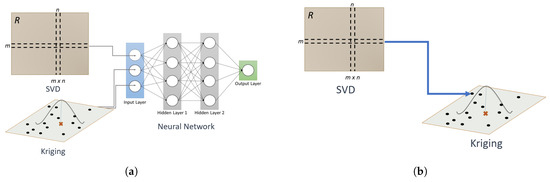
Figure 1.
Combination of SVD and Kriging. (a) Combination of Individual Results [18]; (b) Feeding SVD Results into Kriging.
The technique of using auxiliary attributes of data as independent variables in universal kriging is also referred to as regression kriging (RK). This method has been used extensively in the environmental sciences. The authors of [19] describes different case studies where RK is traditionally applied in the field of environmental science. The study explores mapping soil organic matter using RK, mapping presence/absence of the yew plant, and mapping land surface temperatures. More recently, RK has also been extended to the machine learning field of study. In 2011, a study experimented with using residuals from machine learning into ordinary kriging (OK) [16]. For their combined methods, they applied LM, GLM, GLS, Rpart, RF, SVM and KSVM to the data, then OK or Inverse Distance Squared (IDS) was applied to the residuals of these models. They predicted values of each model and the corresponding interpolated residual values were added together to produce the final predictions of each combined method. The combination of RF and SVM with OK and IDS were novel at the time and had not been applied in previous studies in environmental sciences. In 2015, a study used a similar approach to [16] and applied the output of their neural network as covariates in the universal kriging (UK) algorithm and also applied the neural network residuals as covariates to the ordinary kriging algorithm to interpolate atmospheric temperatures [20]. However, the study found that their approaches were only successful 50% of the time. More recently in 2019, another study used the residuals from the machine learning algorithms Random Forest and Boosted Regression Trees to predict topsoil organic carbon [21]. However, the researchers did not find any significant improvements using the residuals as covariates to OK.
Our approach spatially improves recommender engines using similar approaches in [20,21] but build models for each distinctive region. For our algorithm, truncated SVD is segmented by county and calculated individually. Then, both the outputs and residuals from the collaborative filtering method for each county are used as independent variables in UK. The observed values from truncated SVD are weighted based on the spatial structures calculated from UK, resulting in statistically significant improvements to truncated SVD.
3. Preliminaries
In this section, we discuss the Zillow House Price dataset used for our study and we present the existing concepts exploited by our algorithm used for our approach to combine recommender systems with spatial statistics. By selecting the appropriate hyper-parameters and models within each algorithm, we are able to utilize the strengths of each method to optimize the interpolation of housing estimates.
3.1. Study Area and Dataset
The data used for this study was derived from the Zillow Price Competition on Kaggle in 2016 and can still be found on the Kaggle website (Kaggle Data Set available at: https://www.kaggle.com/c/zillow-prize-1/data). The competition was to develop an algorithm that makes predictions about the future sale prices of homes and in turn help increase the accuracy of the current Zillow algorithm at the time. While the competition has now been closed, we utilized this data set on our algorithm because the data points are densely populated, as shown in Figure 2, which makes it an excellent candidate for testing our algorithm that requires at least a moderate level of spatial autocorrelation.
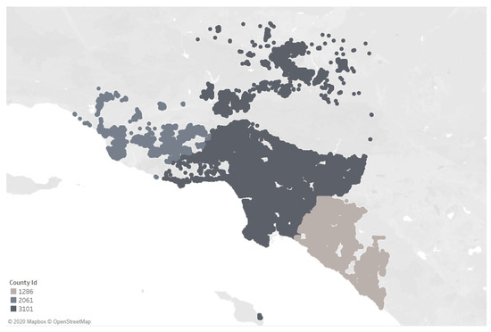
Figure 2.
Zillow Price Competition Data.
The data set contains points from three different counties in California: Ventura, Los Angeles, and Orange county with County ID’s 2061, 3101, and 1286 respectively. Each county will be evaluated to examine what methods are best to predict housing prices based on the characteristics of each county. The data contains dozens of attributes of each home but for this study we selected the attributes that had the least “NA” values which include, latitude, longitude, bedroom count, and bathroom count. Figure 3 provides a boxplot to show the range of housing prices in each of the three counties. The boxes show the 25% to 75% quantiles of housing prices for each county, whereas their whiskers (the lines reaching out from the boxes) show the 2.5% to 97.5% quantiles. We observe that County 3101 has the largest range of house prices, including outliers costing less than USD 1000, and houses priced at as much as ten million USD.
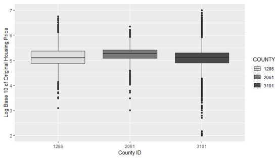
Figure 3.
Boxplot of Housing Prices.
3.2. Ordinary and Universal Kriging
Geostatistics was originally developed from the gold mining industry in the 1950s to determine if the local metal concentrations in ores were sufficient to make the extraction worthwhile. With much success, this method had proven to be an effective way to interpolate values assuming a continuous surface underneath. No model can perfectly describe the natural world and any technique used for interpolation will results in some amount of error. It is here where geostatistics, unlike other methods such as Voronoi polygons or trend surface analysis, is an optimal choice because it can provide estimates of the model errors. Even now, geostatistics is a popular method in environmental sciences [22,23]. Many scientists want to measure properties of interest to them (i.e., nutrients in soil, air pollution, rainfall) over a large continuous areas over which they often have only sparse observed data at limited numbers of places [17]. In these circumstances the best that they can do is to estimate or predict in a spatial sense values between observed points and use geostatistics in this way.
The geostatistics technique kriging is used to interpolate values of non-sampled locations from a collection of sampled areas and estimate the uncertainty surrounding the predicted value [24]. Kriging is not effective if there is no or negative spatial autocorrelation among data points [25]. But for the case of house pricing estimation, the literature provides evidence of spatial auto-correlation [1] confirming Tobler’s first law of geography, stating that “Everything is related to everything else. But near things are more related than distant things.” [26]. For more information on a recent tutorial on kriging can be found at [27]. Following this intuition, we assume that housing prices are spatially autocorrelated, which can be exploited for predicting using a kriging estimate.
Typically, ordinary kriging interpolates values assuming stationarity and homoscedasticity, thus assuming no trend. In other words, the mean and variance across the entire spatial domain is assumed to be constant. This study incorporates Ordinary Kriging which assumes a constant stationary function and is calculated using Definition 1:
Definition 1
(Ordinary Kriging Estimate). The kriging estimate is of the form:
where is the estimated value (specifically, housing prices in our use-case) at location ; are all other observed values at locations ; N is the sample size; and weights chosen for .
The challenging part of Definition 1 is to find appropriate weights to define how much an observed value at location affects the value to be estimated. For this purpose, different models (variograms) are used in the literature to choose the weight depending on the distance between the estimated location and the location of the predictor value .
Definition 2
(Empirical Variogram).
where is the set of experimental pairs having distance h, that is, a set of observations having , and are the observed values at places and + h.
In order to build the appropriate models, kriging builds an empirical Variogram (Definition 2) which is calculated by substituting the distance between two observed points into Definition 2. The empirical variogram values provide information on the spatial autocorrelation of the dataset and can then be used to fit a model to ensure that kriging predictions have positive kriging variances [28]. This data, which has N = 16,997 house prices as described in Section 3.1, leads to = 288,881,012 pairs of data points. These pairs are grouped by their Euclidean distance, and for each distance group at 0.01 mi the corresponding empirical covariance (as defined in Definition 2) is given on the y-axis.
We can empirically observe whether there is a strong spatial autocorrelation within the data based on the empirical variograms, showing at what point the correlation drops and the covariance as distance increases. An experimental variogram that increases with increasing gradient as the lag distance increases signifies trend [17]. When trend is present within the data, the process should be modelled as a combination of a deterministic trend and spatially correlated random residuals from the trend [17]. Thus, for this study we also use Universal Kriging where the mean will differ throughout the spatial domain while still assuming homoscedasticity, i.e., assuming that the variance is constant and is used when data has a strong trend.
To leverage the empirical variogram (Definition 2) for kriging, the values of in Definition 1 are chosen by solving the following set of equations:
where is a model of the semivariance between as defined in Definition 2 given their distance . By definition, the kriging weights are subject to the constraint that they sum to one [17]. is a Lagrange multiplier introduced for the minimization of the error variance, thus must sum to one. Ordinary Kriging assumes a stationary stochastic process, i.e., having a constant (but unknown) mean. But for housing prices, different areas may have different mean house price, depending on neighborhood, school district, and proximity to public transport [2,3,4].
Universal Kriging (UK) is used for non-stationarity when drift is present. It allows for non-stationarity thus allowing the mean to differ throughout the spatial domain while still assuming homoscedasticity, i.e., assuming that the variance is constant and is used when data has a strong trend. UK assumes that the prediction variable, , can be written as a sum of deterministic trend component and the spatially correlated random residual component :
Definition 3
(Universal Kriging).
where is the ith coefficient to be estimated from the data; is the ith basic function of spatial coordinates which describes the drift; k is the number of functions used in modeling the drift; is a spatially correlated random residual.
For this study, the mean, is assumed to have a linear function of two-dimensional coordinates with k = 3 and can be approximated by a suitable model with the form [29]:
where is the coefficient to be estimated from the data, and x and y are the spatial coordinates in formal UK. With the appropriate equations mentioned above, we can calculate an empirical variogram to determine the weights of the observed values. Unlike Ordinary Kriging, where the variances are calculated by the observed location values and , in UK they are calculated by the observed location residuals from the trend. In contrast to the mean in OK which assumes to be constant, the mean in UK is a function of the spatial coordinates and the local drift which is represented by a linear equation of the independent variables.
To build a model of the empirical semivariogram as required in Equation (3) different parametric models can be used. For this study, the Spherical and Matern model were interchangeably chosen since they best fit the empirical semivariogram in different counties. The Spherical model is given by the following expression:
where d is the distance parameter or range, is the nugget variance, c is the variance of spatially correlated component, and h is the lag interval. The Matern model is given by the following expression [30]:
where h is the distance between the observed point and unobserved point, (·) is the modified Bessel function of order , (the “range” parameter) controls the rate of decay of the correlation between observations as distance increases, and controls the behavior of the autocorrelation function for observations that are separated by small distances [31].
3.3. Truncated Singular Value Decomposition (SVD)
Matrix factorization has become the state-of-the-art technique for recommendation systems as popularized by the “Funk” Singular Value Decomposition method used in the 2015 Netflix Challenge [32]. The idea of matrix factorization is to represent a data matrix by multiple (much-) lower dimensionality matrices of latent factors. Then, multiplying of the factorized matrices yields an approximation of the original matrix that allows to estimate missing values within the matrix. The goal of truncated SVD is to keep only the k latent factors having the most information. SVD has also been used to compare ground data and measurements collected by Earth systems because SVD offers an effective method in finding frequent and simultaneous patterns between two spatio-temporal fields [8].
The idea behind such latent factor models is that a large portion of a data matrix R may be highly correlated, and can be approximated by matrices of a lower rank. For example, a matrix that stores a rating value for each of n user combinations, and each of m items may have high redundancy: Some users may be very similar to each other, while some items may exhibit similar reactions to topics.
Definition 4
(Singular Value Decomposition (SVD)).
Let R be a matrix. SVD factorizes R into three components:
where U is a matrix, V is a matrix, and Σ is a diagonal matrix containing the singular values of R in descending magnitude. Intuitively, Σ can be seen as a scaling matrix, that scales dimensions according to their variance/information. U and V can be seen as rotation matrices, which rotate the data space in the directions of the highest variance components.
The idea of truncated SVD is to simply truncate all but the k highest variance components, discarding the rest of the matrices. This not only allows for an efficient approximation of R, but it also allows to discard detailed and potentially overfitting information.
Definition 5
(Truncated SVD). Let R be a matrix and let . Truncated SVD factorizes R into three components:
where is a matrix, describing each line of R by k latent features, is a matrix, describing each column of R by k latent features, and is a diagonal matrix retaining the largest singular values of Σ. Σ can be seen as a scaling matrix, that scales dimensions according to their variance/information. U and V can be seen as rotation matrices, which rotate the data space in the directions of the highest variance components.
The matrix factorization method provides a clear way to observe the correlations between rows and columns in a one-shot estimation to the entire matrix [33]. To leverage this factorization for prediction, we rebuild an approximation of data matrix R, by multiplying the truncated matrices. In the resulting matrix, each predicted value, , in is calculated by the dot product of the ith row factor of and the jth column factor of [33]:
Once the latent vectors for rows and columns are established, it is simple to use Equation (10) for estimating the values of R. Since SVD cannot directly compute estimates with an incomplete matrix, a simple approach is to take the average of the columns or rows of the observed values and input them into the missing ratings. However, this approach can be biased. By using the truncated SVD algorithm with Stochastic Gradient Descent (SGD) which is a convex optimization method, only observed values will be taken into consideration while avoiding overfitting through a regularized model [32]. Overfitting is common when a training dataset is small. Through regularization, the models incorporate a bias which discourages extremely large values of the and coefficients to promote stability. SGD is used in truncated SVD as an approach to minimize error by finding at what point the slope of the error loss function is closest to zero by looping through all observed values, computing the prediction error, and then using the error from each observed value to update the k entries in row i of U and k entries in column j of V. Details of this SGD approach for approximating missing values in truncated SVD can be found in [32,33,34].
While truncated SVD has proven its predictive power in many applications such as user-movie recommendation [35] and face recognition [36], it does not explicitly allow to model spatial locations and spatial auto-correlation. This limitation is evident due to truncated SVD using linear algebra only, which is too limited to describe spatial trends. Therefore, in the following, we propose a modification to kriging which augments the power of latent factor modeling using truncated SVD with a kriging approach that gives spatial information appropriate special treatment.
4. Methodology
In this study, with the Zillow data discussed in Section 3.1, we first show that ordinary kriging can provide better house price prediction better than machine learning approaches based on SVD. As shown in Figure 4, if the variogram for a specific couny fits the data well, than ordinary kriging in the method of choice. However, if trend is present in the variogram, than our algorithm SVD-RK can enhance ordinary kriging by generating stronger predictions.
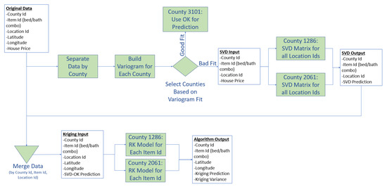
Figure 4.
Methodology Flowchart.
In a nutshell, the idea of our approach is to first assess how well the deviation of prices can be explained by distance. Cases where the covariance function shows a strong fit to the empirical variogram indicate that that ordinary kriging may be sufficient to yield good predictions, without the need to further explain the deviation using SVD. However, in cases where some places cannot be explained by their local neighborhoods, such as an expensive area adjacent to cheaper housing, or areas in close proximity having varying house prices due to different school districts, we may be able to leverage SVD. The idea is that SVD may find that a location is similar to other areas (regardless of distance), and thus, estimate house prices similar to these locations having similar (latent) features. The following subsection describes our approach, as shown in Figure 4, to leverage universal kriging with information derived from latent feature analysis using truncated SVD.
4.1. Step 1: Segmenting
Our proposed algorithm integrates hidden patterns that the human eye cannot detect using distance and spatial arrangement of nearby observations to improve the prediction of unobserved values. In a previous study [18], we combined the outputs of SVD and OK into a hybrid model using a multi-linear regression model and a neural network as shown in Figure 1a. The shortcoming of this approach is the assumption of a stationary data set, where mean and standard deviation of the variable of interest are identical in all locations. This assumption held in the previous study [18], of predicting emotion values rather than house prices. However, different neighborhoods can have significantly different mean house prices, incurring a large error if stationary means and homoscedasticity are assumed, and leading to major confusion by the neural network approach as shown in Table 1.

Table 1.
Mean Absolute Error (MAE) in USD for baseline approaches, including Ordinary Kriging (OK), Universal Kriging (UK), Singular Value Decomposition (SVD), and the Hybrid Algorithm presented in [18].
Table 1 also shows us that when the whole data set is ingested into SVD, UK, and OK, then SVD outperforms both types of kriging significantly. However, as shown in the second row of Table 1, when the data is segmented by county, OK performs better than when the whole data set is utilized at once. This is because, when segmented, each county has its own covariance function that describes the unique spatial auto-correlation. We leverage this segmentation for both SVD matrices and kriging models, and build an algorithm that can outperform both SVD and kriging. Thus, as shown as in Figure 4, the first step from the Original Data is to separate the data by county.
4.2. Step 2: Variogram Construction
In the second step of Figure 4, we take the separated data and construct house pricing variograms for each study area to understand their spatial structure. The purpose of the variogram for a study area is to decide whether kriging alone is expected to yield good predictions, or if we should leverage SVD to explain the unexplained residuals which is the decision point in Figure 4. Our experimental evaluation in Section 5 will depict example cases in which the model variogram strongly fits the empirical variogram such that SVD cannot improve the housing prediction (county id 3101), and show cases in which the model variogram does not fit the empirical variogram well such that the strength of SVD can improve the housing price prediction (county id 1286 and 2061).
4.3. Step 3: Applying SVD to House Price Matrix
In order to utilize truncated SVD as part of our algorithm, we used location ids that were derived from unique latitude and longitude combinations as the rows for the matrix, and the non-spatial attributes (bedroom and bathroom combinations) for the columns of the matrix as shown in Figure 5. This data structure allows the truncated SVD algorithm to make housing price predictions of different locations for all the possible bedroom-bathroom possibilities that were unavailable, depicted in orange cells in Figure 5. Truncated SVD allows our algorithm to leverage the benefits of traditional recommender systems by identifying similar locations (i.e., locations having similar prices for the similar types of houses), and by identifying similar types of houses (i.e., types of houses having similar prices for similar locations). Truncated SVD only takes into consideration hidden patterns within the data and does not look at spatial elements in any way. Our approach is designed to use the SVD outputs and residuals and weigh the truncated SVD predictions based on their spatial structure through RK, which we call SVD-RK.
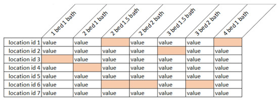
Figure 5.
Housing Price Matrix Representation.
4.4. Step 4: Feeding Truncated SVD into Regression Kriging
As described in Figure 4, kriging and SVD are combined by feeding the SVD output into a regression kriging as covariates as sketched in Figure 1b and architected in Figure 4. The reason for feeding SVD outputs into kriging instead of kriging outputs into SVD is because in real estate housing price estimation, the SVD outputs are stronger than UK when compared individually as shown in Table 1. Thus, feeding more accurate estimations from SVD into kriging, our algorithm will further improve the predictions by taking into account spatial autocorrelation.
The idea of our approach is that truncated SVD leverage latent features of locations for prediction. For example, SVD may find that one location exhibits similar housing prices than a set of other locations, thus leveraging these other locations for prediction. Truncated SVD treats each location as a nominal variable, and thus, is oblivious of distances between locations and unable to leverage spatial autocorrelation. By leveraging the variogram constructed as described in Section 4.2 (and shown in Section 5 for the Zillow dataset described in Section 3.1), we can explore if a given dataset is strongly spatially autocorrelated. In that case, we use the unobserved values estimated by trunacated SVD as independent variables for universal kriging (UK). Traditionally, the mean of UK is a function of the site coordinates, such that the latitude and longitude are independent variables of a linear model [17]. However, UK can also use a regression from other independent variables which is known as regression kriging (RK). RK is a spatial interpolation technique that combines a regression of the dependent variable on auxiliary variables (such as soil nutrients, or temperature) with simple kriging of the regression residuals. It is mathematically equivalent to the UK, where auxiliary predictors are used directly to solve the kriging weights [19]. Instead of using latitude and longitude as traditional auxiliary variables, we use other attributes, the SVD outputs and residuals, as independent variables which lead to better results. This allows UK to use new auxiliary variables to calculate the weight matrix for all observed points. The study [20] explored regression kriging using the outputs of an artificial neural network as covariates to UK. The approach showed some promising properties, in that it did better than UK alone in four out of eight examined model cases, however, the evidence of benefits was inconclusive since it showed varying degrees of success. In the study [21], Random Forest and Boosted Regression Tree residuals were used as covariates with ordinary kriging but RT residuals with OK did not show any improvements as covariants. The study found that OK and UK were the most accurate mapping methods in comparison to RK. We experimented using the truncated SVD outputs and the truncated SVD residuals as covariates separately for OK and UK. However, we found that that these methods, as explained in [20,21] showed no benefit in predicting points. Thus we applied a segmentation enhancement to the approach that has shown strong improvements to the final predictions.
The strength of kriging is that a variance can be calculated to determine the certainty of the kriging interpolation. SVD-OK feeds SVD into kriging which not only outputs a stronger prediction than either SVD or kriging individually, but it also outputs a variance. This can be utilized to make intelligible predictions because it quantigies the confidence of the prediction that the algorithm makes. Thus the variance causes a more explainable approach to machine learning. Another important aspect to UK is that the technique is able to calculate the weight vector for unobserved points using independent variables that may only be present in training the model but not present or available in the unobserved points. With this in mind, we have utilized both the truncated SVD output and the truncated SVD residual as independent variables together in creating our covariance function. Thus, the kriging approach not only knows the SVD prediction based on latent factors, but it also knows the confidence of these prediction given its difference to the ground truth of training data. Our results show that our combined approach SVD-RK, which feeds the truncated SVD results in regression kriging outperforms individual approaches based on matrix factorization and kriging alone as well as the approaches in previous studies [20,21].
4.5. Coding Language and Packages
This study was conducted using both the R and Python programming languages. The python package “surprise” was used to apply truncated SVD to the data. Specifically the NMF function, under the matrix factorization algorithms, within the “surprise” package was used to to perform truncated SVD. This function ensures that the user and item vectors stay positive. More information on this technique can be found in [37,38]. For this function, Table 2 describes the hyperparameters used for this study. The R package “gstat” was used in applying kriging to the data. The “variogram”, “fit.variogram”, and “krige” functions were utilized in making the predictions using the truncated SVD outputs and residuals. All code for this study can be found on on GitHub [39].
Table 2.
SVD Hyperparamter Values.
5. Experimental Evaluations
Our aim is to explore and combine the techniques of kriging and Recommender Engines using truncated SVD such that the results will stabilize and reduce the mean absolute error (MAE) of housing price predictions. In order to leverage the strengths of both methods, we first built variograms for each county. Each county describes a different spatial structure as shown in Figure 6. As shown with Figure 6a, the covariance function fits the empirical variogram very well for county id 3101 which gives us insight into what algorithm to use for this county. Since the covariance function can describe the spatial structure well for county id 3101, OK will be the most suitable approach to predicting housing prices. As shown with Figure 6b,c, the best fit curve function still cannot fully describe the spatial structure for county id 1286 and 2061. However, with our proposed algorithm, we found that SVD-RK can utilize hidden patterns within the data and kriging can weigh the SVD outputs and residuals based on spatial correlation to produce stronger results than OK alone.
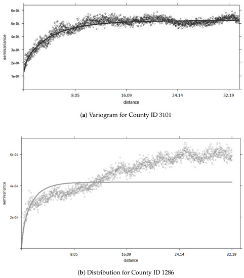
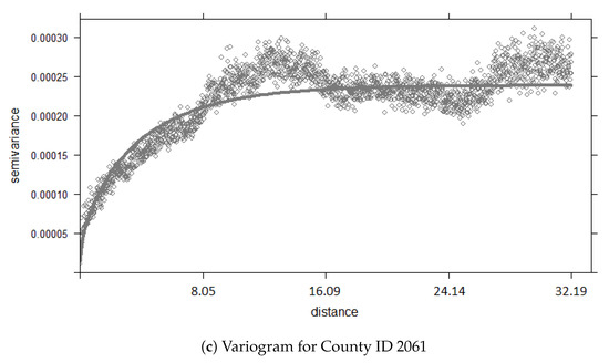
Figure 6.
Empiracle Variograms (in kilometers).
For the experiments conducted, we split the data into training and testing sets. Since the data was derived from the Zillow Kaggle Challenge as explained in Section 3.1, the challenge specified which data points were to be used as part of the training and testing. This study followed the exact same train/test split procedure for the purpose of producing comparable results. Following the exact same procedure allows all the experiments in this study to be evaluated fairly. In addition, there were no issues with minimum point density as a limitation for kriging. Since the data has already been pre-processed for the Kaggle challenge, there was a sufficient amount of points to build a variogram for every county. Furthermore, for data points that had NA values for some attributes, these lines of data were dropped. Only values within the data set that had a value for latitude, longitude, bedroom count, bathroom count, and price were utilized in this study.
5.1. Evaluation of SVD-RK
Integrating truncated SVD into regression kriging, we first created separate matrices for each county to find the latent patterns. An important SVD parameter is the choice of K, the number of latent features, shown in Table 2. From running experiments shown in Figure 7, we found that any number less than 10 features yields similarly good prediction results. In particular, we get similar (only slightly worse results) using latent features instead of . This shows that a single feature (which may latently describe the “priceliness” of a neighborhood) yields good price prediction results.
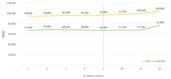
Figure 7.
Latent Factor Experiment.
Table 2 also shows the appropriate amount of epochs, which is the number of iterations of the SGD procedure. The learning rate in SVD is the average rating given by a user minus the average ratings of all items. This term is used to reduce the error between the predicted and actual value. For this study, the learning rate set to 5 × 10 was found to produce optimal results.
The SVD results are then fed into separate kriging models by county to weigh the observed values based on the spatial description of that county. Since every county may have different characteristics, segmenting the models helps to weigh the observations appropriately.
As shown in Table 3, our method, SVD-RK, which applies truncated SVD matrices and kriging models by region presents improvements to counties 1286 and 2061, which could not be fully described by the covariance function in kriging alone as shown in Figure 6. We found that when appling SVD-RK to each county reperately, truncated SVD matrices are able to better learn the hidden features of the data for a particular area thus producing results with less outliers which leads to better kriging results. For truncated SVD, every county may have different hidden characteristics which can be extracted more clearly when segmented. For UK, segmenting each model by county, in addition to segmenting matrices in truncated SVD, allows the algorithm to better describe the spatial structure of each county better than apply one generic covariance function to describe all three counties. Thus, applying SVD-RK by county, allows the algorithm to tailor the spatial structure differently for a given area. One area may be best described with a Spherical covariance function while another may be better described with a Matern covariance function. Table 4 lists the spatial structure for each county to highlight their differences and why segmenting would stabilize the results and make better predictions for certain counties.
Table 3.
Segmenting SVD Matrices and Kriging.
Table 4.
Spatial Structure by County.
For comparison purposes we also tested how Non-Negative Matrix Factorization (NMF), an implementation for SVD that follows [38], would react if fed into RK. NMF is similar to SVD, except for having an additional constraint of imposing non-negative weights in matrices U and V. Table 3 shows the results of NMF-RK and show that SVD-RK yields better results. Thus this study focuses on SVD-RK as the method of choice.
Our approach, as shown in Table 3, does not work well for county 3101, which covers regions of different densities with large distances between these regions (see Figure 2), which also has outliers with extremely low/high house prices, as shown in Figure 3. In this case, the large variance of house prices combined with the large distance to nearest points in some locations yields to vast mis-estimations. We also see that ordinary kriging yields extremely good results for this county, due to the variogram fitting the empirical covariances very closely as shown in Figure 6a. Thus, in this case, the spatial location (captured by orginary kriging) is already able to tightly fit the data and explain most of the error. Yet, we will propose two approaches to improve our approach to work in cases such as County 3101. First, we will propose an approach for outlier remove in Section 5.2. While this appraoch stabilizes our SVD-RK approach, it still yields worse results than ordinary kriging. Thus, we propose to substitute regression kriging with geographically weighted regression (GWR), in our approach, leading to better results in Section 5.3.
5.2. Outlier Removal for SVD-RK
While SVD-RK has shown significant improvements to the truncated SVD predictions, county id 3101 had no improvement. To better understand why the improvement for county id 3101 was not as strong as the others, we created a boxplot to visually see the outliers in Figure 3 and mapped the housing prices shown in Figure 8. Figure 8a shows county id 3101 with a relatively even distribution of housing price values except near the bend where there are red housing prices showing more extreme values, while Figure 8b for county id 2061 and 1286 shows almost no extreme values. We then calculated the minimum, maximum, average, and standard deviation of the housing prices for each county id shown in Table 5. From Table 5, it is evident that county id 3101 has the largest difference between the minimum and maximum house price points and has visible outliers. Since kriging is highly sensitive to skewed distributions and extreme positive values having a large impact on semi-variance calculations, this caused the improvement in error to be relatively smaller for county id 3101 [17].
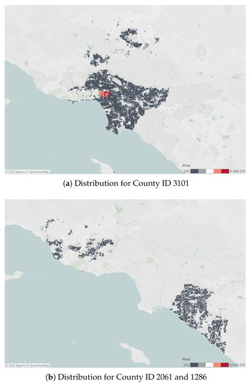
Figure 8.
Data Distribution.
Table 5.
Price Distribution by County in One Thousand USD.
To improve the mean absolute error for county id 3101, we proposed removing the outliers when kriging to decrease standard deviation and range between the maximum and minimum values. We removed all outliers deviating by more than two standard deviations from the mean. This resulted in a smaller standard deviation and an increase in accuracy by 25.9% (shown in Table 6) from the original segmentation OK method (shown in Table 3). For those outliers that were left from being ingested into the algorithm, the results from using OK without treating outliers can still be used with an MAE of 83,000.
Table 6.
Removing Outliers for County Id 3101.
5.3. Feeding Truncated SVD into Geographically Weighted Regression (SVD-GWR)
In addition to non-stationary kriging, this study also explored improving truncated SVD with Geographically Weighted Regression (GWR) since it is one of the recent developments of spatial analytical methods [40]. GWR is a local spatial statistical technique for exploring non-stationary data and, although controversial, it can also be used to make predictions. Similar to kriging, this algorithm is closely related to Tobler’s first law of geography assuming that closer observations are more related than distant observations [26]. GWR calibrates a separate ordinary least squares regression at each location in the data set within a certain bandwidth and allows the relationships between the independent and dependent variables to vary locally. The GWR model can be described as the following:
where is the dependent variable at location i, is the intercept coefficient at location i, is the k-th explanatory variable at location i, is the k-th local regression coefficient for the kth explanatory variable at location i, is the random error term associated with location i, and i is indexed by two-dimensional geographic coordinates [41]. The equation for GWR is similar to traditional regression however, for GWR, the regression coefficients are estimated at each data location rather than being fixed for a study area [40]. Further details for the GWR method can be found in [40,41,42,43].
While some studies have shown the potential of GWR as a predictor [44] there is still some controversy whether to use this method to make predictions [45]. Thus we compared GWR to OK for county id 3101 and our algorithm SVD-RK for county id’s 1286 and 2061 to determine if this method would increase the prediction accuracy better. For this experiment we used the truncated SVD output and residual as independent variables for Equation (11). Table 7 shows the results of applying integrating truncated SVD to GWR, which we called SVD-GWR, compared to the OK algorithm (since this method performed the best for county id 3101 as seen in Table 3). We found that SVD-GWR improves the accuracy by 6.2%. However, Table 8 shows that SVD-GWR performed worse for county id 1286 and 2061 in comparison to SVD-RK (the optimal method for the two counties as shown in Table 3).
Table 7.
GWR over OK in USD.
Table 8.
GWR over SVD-RK in USD.
Since removing outliers for county id 3101 improved the OK method (shown in Table 6), we also wanted to determine if removing outliers would improve the SVD-GWR method. Table 9 shows that there was an improvement to the error in comparison to SVD-GWR without being treated for outliers, however the improvement of OK treated with outliers in Table 6 is still the method that produced the lowest error for county id 3101.
Table 9.
GWR over OK without Outliers in USD.
6. Conclusions and Future Work
Housing price estimation is a challenging task that depends not only on properties of a house, but also on its location. We propose a system that leverages the predictive power of a latent-feature based recommender engine using truncated singular value decomposition (SVD). As such systems are spatially oblivious, we integrate the result into regression kriging. This way, kriging fits a model to a data set in which gaps are filled by SVD, and where outliers, which cannot be explained by the main latent features of the data, are removed by truncation of non-principal components of SVD. Our experimental evaluation shows that our proposed integrated approach SVD-RK outperforms both standalone SVD, standalone ordinary kriging, and universal kriging in two out of three study areas where the variogram fit shows a degree of trend. However, for the study area that has a good variogram fit a straightforward application of our proposed approach may fail. Therefore, we propose to augment our approach using an outlier detection approach, as well as combining it with GWR to better account for outliers in the data.
Our work shows that, given only basic information about houses such as the number of rooms and bathrooms, the combination of SVD and kriging yields the best of both worlds of recommender systems and spatial interpolation. A next step of this work is consider further non-spatial features, such as the size of a house (in square meters), and the age of house (in years), in the recommender system module to give SVD a more accurate prediction, and thus, improve the SVD-RK result.
Author Contributions
Conceptualization, Aisha Sikder and Andreas Züfle; methodology, Aisha Sikder and Andreas Züfle; software, Aisha Sikder; validation, Aisha Sikder and Andreas Züfle; formal analysis, Aisha Sikder and Andreas Züfle; investigation, Aisha Sikder and Andreas Züfle; resources, Andreas Züfle; data curation, Aisha Sikder; writing—original draft preparation, Aisha Sikder and Andreas Züfle; writing—review and editing, Aisha Sikder and Andreas Züfle; visualization, Aisha Sikder; supervision, Andreas Züfle; project administration, Aisha Sikder and Andreas Züfle; funding acquisition. All authors have read and agreed to the published version of the manuscript.
Funding
This research received no external funding.
Conflicts of Interest
The authors declare no conflict of interest.
Abbreviations
The following abbreviations are used in this manuscript:
| OK | Ordinary Kriging |
| RK | Regression Kriging |
| SVD | Singular Value Decomposition |
| SGD | Stochastic Gradient Descent |
| UK | Universal Kriging |
| MAE | Mean Absolute Error |
References
- Gibbons, S.; Machin, S. Valuing school quality, better transport, and lower crime: Evidence from house prices. Oxf. Rev. Econ. Policy 2008, 24, 99–119. [Google Scholar] [CrossRef]
- Haurin, D.R.; Brasington, D. School quality and real house prices: Inter-and intrametropolitan effects. J. Hous. Econ. 1996, 5, 351–368. [Google Scholar] [CrossRef]
- Adair, A.; McGreal, S.; Smyth, A.; Cooper, J.; Ryley, T. House prices and accessibility: The testing of relationships within the Belfast urban area. Hous. Stud. 2000, 15, 699–716. [Google Scholar] [CrossRef]
- Lynch, A.K.; Rasmussen, D.W. Measuring the impact of crime on house prices. Appl. Econ. 2001, 33, 1981–1989. [Google Scholar] [CrossRef]
- Duca, J.V.; Muellbauer, J.; Murphy, A. Housing markets and the financial crisis of 2007–2009: Lessons for the future. J. Financ. Stab. 2010, 6, 203–217. [Google Scholar] [CrossRef]
- Das, J.; Majumder, S.; Gupta, P. Spatially aware recommendations using kd trees. In Proceedings of the Third International Conference on Computational Intelligence and Information Technology (CIIT 2013), Mumbai, India, 18–19 October 2013. [Google Scholar]
- Bohnert, F.; Schmidt, D.F.; Zukerman, I. Spatial processes for recommender systems. In Proceedings of the Twenty-First International Joint Conference on Artificial Intelligence, Pasadena, CA, USA, 14–17 July 2009. [Google Scholar]
- Bogaardt, L.; Goncalves, R.; Zurita-Milla, R.; Izquierdo-Verdiguier, E. Dataset reduction techniques to speed up svd analyses on big geo-datasets. ISPRS Int. J. Geo-Inf. 2019, 8, 55. [Google Scholar] [CrossRef]
- Cellmer, R. The possibilities and limitations of geostatistical methods in real estate market analyses. Real Estate Manag. Valuat. 2014, 22, 54–62. [Google Scholar] [CrossRef]
- Kuntz, M.; Helbich, M. Geostatistical mapping of real estate prices: An empirical comparison of kriging and cokriging. Int. J. Geogr. Inf. Sci. 2014, 28, 1904–1921. [Google Scholar] [CrossRef]
- Pace, R.K.; Barry, R.; Sirmans, C.F. Spatial statistics and real estate. J. Real Estate Financ. Econ. 1998, 17, 5–13. [Google Scholar] [CrossRef]
- Zhou, X.; Tong, W.; Li, D. Modeling Housing Rent in the Atlanta Metropolitan Area Using Textual Information and Deep Learning. ISPRS Int. J. Geo-Inf. 2019, 8, 349. [Google Scholar] [CrossRef]
- Yang, D.; Zhang, D.; Zheng, V.W.; Yu, Z. Modeling User Activity Preference by Leveraging User Spatial Temporal Characteristics in LBSNs. IEEE Trans. Syst. Man Cybern. Syst. 2015, 45, 129–142. [Google Scholar] [CrossRef]
- Wang, W.; Yin, H.; Sadiq, S.; Chen, L.; Xie, M.; Zhou, X. SPORE: A sequential personalized spatial item recommender system. In Proceedings of the 2016 IEEE 32nd International Conference on Data Engineering (ICDE), Helsinki, Finland, 16–20 May 2016; pp. 954–965. [Google Scholar]
- Yang, G.; Züfle, A. Spatio-Temporal Site Recommendation. In Proceedings of the 2016 IEEE 16th International Conference on Data Mining Workshops (ICDMW), Barcelona, Spain, 12–15 December 2016; pp. 1173–1178. [Google Scholar]
- Li, J.; Heap, A.D.; Potter, A.; Daniell, J.J. Application of machine learning methods to spatial interpolation of environmental variables. Environ. Model. Softw. 2011, 26, 1647–1659. [Google Scholar] [CrossRef]
- Oliver, M.A.; Webster, R. Basic Steps in Geostatistics: The Variogram and Kriging; Springer: New York, NY, USA, 2015; Volume 106. [Google Scholar]
- Sikder, A.; Züfle, A. Emotion predictions in geo-textual data using spatial statistics and recommendation systems. In Proceedings of the 3rd ACM SIGSPATIAL International Workshop on Location-Based Recommendations, Geosocial Networks and Geoadvertising, Chicago, IL, USA, 5 November 2019; p. 5. [Google Scholar]
- Hengl, T.; Heuvelink, G.B.; Rossiter, D.G. About regression-kriging: From equations to case studies. Comput. Geosci. 2007, 33, 1301–1315. [Google Scholar] [CrossRef]
- Tadić, J.M.; Ilić, V.; Biraud, S. Examination of geostatistical and machine-learning techniques as interpolators in anisotropic atmospheric environments. Atmos. Environ. 2015, 111, 28–38. [Google Scholar] [CrossRef]
- Veronesi, F.; Schillaci, C. Comparison between geostatistical and machine learning models as predictors of topsoil organic carbon with a focus on local uncertainty estimation. Ecol. Indic. 2019, 101, 1032–1044. [Google Scholar] [CrossRef]
- Trangmar, B.B.; Yost, R.S.; Uehara, G. Application of geostatistics to spatial studies of soil properties. Adv. Agron. 1986, 38, 45–94. [Google Scholar]
- Sigua, G.C.; Hudnall, W.H. Kriging analysis of soil properties. J. Soils Sediments 2008, 8, 193. [Google Scholar] [CrossRef]
- Zhou, H. Computer Modeling for Injection Molding: Simulation, Optimization, and Control; Wiley: Hoboken, NJ, USA, 2012. [Google Scholar]
- Columbia University Mailman School of Public Health. Population Health Methods: Kriging. Available online: https://www.mailman.columbia.edu/research/population-health-methods/kriging (accessed on 24 April 2019).
- Tobler, W.R. A computer movie simulating urban growth in the Detroit region. Econ. Geogr. 1970, 46, 234–240. [Google Scholar] [CrossRef]
- Züfle, A.; Trajcevski, G.; Pfoser, D.; Renz, M.; Rice, M.T.; Leslie, T.; Delamater, P.; Emrich, T. Handling uncertainty in geo-spatial data. In Proceedings of the 2017 IEEE 33rd International Conference on Data Engineering (ICDE), San Diego, CA, USA, 19–22 April 2017; pp. 1467–1470. [Google Scholar]
- How Kriging Works. 2019. Available online: http://desktop.arcgis.com/en/arcmap/10.3/tools/3d-analyst-toolbox/how-kriging-works.htm (accessed on 24 April 2019).
- Zhang, C.; Pei, H. Oil spills boundary tracking using universal kriging and model predictive control by uav. In Proceedings of the 11th World Congress on Intelligent Control and Automation, Shenyang, China, 29 June–4 July 2014; pp. 633–638. [Google Scholar]
- Matérn, B. Spatial Variation; Springer Science & Business Media: Berlin, Germany, 2013; Volume 36. [Google Scholar]
- Hoeting, J.A.; Davis, R.A.; Merton, A.A.; Thompson, S.E. Model selection for geostatistical models. Ecol. Appl. Publ. Ecol. Soc. Am. 2006, 16, 87–98. [Google Scholar] [CrossRef]
- Koren, Y.; Bell, R.; Volinsky, C. Matrix Factorization Techniques for Recommender Systems. Computer 2009, 42, 30–37. [Google Scholar] [CrossRef]
- Aggarwal, C.C. Recommender Systems—The Textbook; Springer: Berlin/Heidelberg, Germany, 2016. [Google Scholar] [CrossRef]
- Bottou, L. Large-scale machine learning with stochastic gradient descent. In Proceedings of COMPSTAT’2010; Springer: Berlin/Heidelberg, Germany, 2010; pp. 177–186. [Google Scholar]
- Bennett, J.; Lanning, S. The netflix prize. In Proceedings of the KDD Cup and Workshop, New York, NY, USA, 12 August 2007; Volume 2007, p. 35. [Google Scholar]
- Zhang, Q.; Li, B. Discriminative K-SVD for dictionary learning in face recognition. In Proceedings of the 2010 IEEE Computer Society Conference on Computer Vision and Pattern Recognition, San Francisco, CA, USA, 13–18 June 2010; pp. 2691–2698. [Google Scholar]
- Lee, D.D.; Seung, H.S. Algorithms for non-negative matrix factorization. In Proceedings of the NIPS 2001 Advances in Neural Information Processing Systems, Vancouver, BC, Canada, 3–8 December 2001; pp. 556–562. [Google Scholar]
- Luo, X.; Zhou, M.; Xia, Y.; Zhu, Q. An efficient non-negative matrix-factorization-based approach to collaborative filtering for recommender systems. IEEE Trans. Ind. Inform. 2014, 10, 1273–1284. [Google Scholar]
- Sikder, A. svd_kriging Github Repository. 2019. Available online: https://github.com/datadj28/svd_kriging (accessed on 24 April 2019).
- Murayama, Y. Progress in Geospatial Analysis; Springer Science & Business Media: Berlin, Germany, 2012. [Google Scholar]
- Oshan, T.M.; Li, Z.; Kang, W.; Wolf, L.J.; Fotheringham, A.S. mgwr: A Python implementation of multiscale geographically weighted regression for investigating process spatial heterogeneity and scale. ISPRS Int. J. Geo-Inf. 2019, 8, 269. [Google Scholar] [CrossRef]
- Harris, P.; Fotheringham, A.S.; Juggins, S. Robust geographically weighted regression: A technique for quantifying spatial relationships between freshwater acidification critical loads and catchment attributes. Ann. Assoc. Am. Geogr. 2010, 100, 286–306. [Google Scholar] [CrossRef]
- Fischer, M.M.; Getis, A. Handbook of Applied Spatial Analysis: Software Tools, Methods and Applications; Springer Science & Business Media: Berlin, Germany, 2010. [Google Scholar]
- Harris, P.; Fotheringham, A.; Crespo, R.; Charlton, M. The use of geographically weighted regression for spatial prediction: An evaluation of models using simulated data sets. Math. Geosci. 2010, 42, 657–680. [Google Scholar] [CrossRef]
- Columbia University Mailman School of Public Health. Geographically Weighted Regression. Available online: https://www.mailman.columbia.edu/research/population-health-methods/geographically-weighted-regression (accessed on 24 April 2019).
© 2020 by the authors. Licensee MDPI, Basel, Switzerland. This article is an open access article distributed under the terms and conditions of the Creative Commons Attribution (CC BY) license (http://creativecommons.org/licenses/by/4.0/).