Abstract
This paper presents an approach to detecting patterns in a three-dimensional context, emphasizing the role played by the local geometry of the surface model. The core of the associated algorithm is represented by the cosine similarity computed to sub-matrices of regularly gridded digital surface/canopy models. We developed an accompanying software instrument compatible with a GIS environment which allows, as inputs, locations in the surface/canopy model based on field data, pre-defined geometric shapes, or their combination. We exemplified the approach for a study case dealing with the locations of scattered trees and shrubs previously identified in the field in two study sites. We found that the variation in the pairwise similarities between the trees is better explained by the computation of slopes. Furthermore, we considered a pre-defined shape, the Mexican Hat wavelet. Its geometry is controlled by a single number, for which we found ranges of best fit between the shapes and the actual trees. Finally, a suitable combination of parameters made it possible to determine the potential locations of scattered trees. The accuracy of detection was equal to 77.9% and 89.5% in the two study sites considered. Moreover, a visual check based on orthophotomaps confirmed the reliability of the outcomes.
1. Introduction
Nowadays, high resolution data encapsulating information regarding the vertical structure, such as elevation, surface, or canopy models derived from point clouds, have become more and more accessible. This calls for methods relying on 3D data and for suitable 3D approaches [1] enabling the detection of fine-scale landscape or vegetation patterns [2]. Such methods can complement state-of-the-art methods of vegetation classification [3,4] or can be used in a synergistic manner, such as the techniques of fusing LiDAR (Light Detection and Ranging) and multispectral imagery [5,6]. The 3D framework makes it possible to separate bare ground and canopy from LiDAR [7] and to explore characteristics of the vertical structure of the canopy cover [8] that were neglected for a long time. Thus, various canopy metrics related to the three-dimensional vegetation structure were brought to our attention: canopy height [9] and crown dimensions [10], the number of trees and tree heights [11], the dendrometric parameters of species [12], or comprehensive sets of forest stand structural parameters [13]. Moreover, such canopy metrics were applied to the classification of the vegetation structure [14]. Another application of the 3D approach was the automatic or semi-automatic detection of specific vegetation features [15] regarded as structural elements of the three-dimensional vegetation cover [16]. The methods based on the three-dimensional representation can be used in a complementary manner, since their performances depend on the type of forest under consideration [17,18].
There are other problems related to vegetation features that might be addressed in the 3D framework. They refer to important small-scale landscape elements [19] such as shelterbelt trees, hedgerows, or scattered trees. The latter are prominent landscape features [20] and represent a defining element of specific vegetation mosaics [21]. Moreover, they play a key role in the provision of ecosystem services and therefore represent a vegetation feature that should be taken into account for future landscape design strategies [22]. In this context, the identification of scattered trees from remote sensing data could be useful for foresters, managers, and landscape planners. On the other hand, by taking into account the scale at which they occur, a reliable approach could be based on high resolution data encompassing the vertical structure, such as high-resolution canopy height models [23].
The identification of vegetation elements by using the 3D geospatial approach could be, in turn, linked to landscape ecological topics such as ecological connectivity, since isolated trees could contribute to a more functional connectivity [24]. For instance, in vegetation mosaics such as wood-pasture landscapes, the scattered trees or the small forest patches provide food resources and facilitate the interconnectivity of the habitats for various species [25,26]. On the other hand, recent studies highlighted that for vegetation mosaics with a variable canopy height, the three-dimensional framework makes it possible to speak about the 3D ecological connectivity which augments the one relying on standard two-dimensional data, since it also refers to the structure of the vegetation strata [27].
Many approaches to identifying landscape or vegetation features in 3D data rely on the use of statistical tools [12,13] or include a pixel-centered approach suitable for the two-dimensional set-up [15]. Although very effective and efficient, such methods pay less attention to the 3D geometry of the objects of interest. We propose an approach that could enhance the existing ones by regarding the regular grids as discrete signals, reformulating the problem of identifying specific 3D patterns as a pattern recognition task and transferring approaches of this field or of related disciplines such as image or signal processing. For instance, multiresolution analysis is a technique for image processing, decomposition, and representation that analyzes the image data at different resolutions or scales without losing information [28]. The signals can be considered in the discrete domain as sequences, or in the continuous domain as functions [29]. The interplay between continuous and discrete is important, since through a discretization process, techniques stemming from the theory of continuous signals could be applied to the discrete ones. An example is provided by the wavelets, which are multi-resolution analysis tools that have emerged as an important tool for signal processing applications [30]. Wavelet methods have been successfully used in the fine scale analysis of a wide range of ecological phenomena [31,32], including landscape pattern and heterogeneity studies [33,34,35,36], ecological modelling [37,38,39], species ecology [40,41,42], and environment analyses [43,44,45,46].
Wavelets come in various shapes; in consequence, each type is useful in analyzing particular data features. In ecological applications, the best known are the Haar wavelet, used for boundary detection [47,48], and the Mexican Hat wavelet. The latter represents a very appealing shape due to its resemblance to a tree, since it has a single central peak and symmetric lateral sides. In reality though, trees often have very disparate shapes and cannot perfectly match a symmetric pre-defined model. One workaround for addressing this issue is the possibility of varying the shape of the Mexican Hat wavelet by adapting the dilation coefficient that controls its geometry and the window size in order to better approximate the tree shape. In this context, the Mexican Hat wavelet has already been used for landscape feature extraction, such as trees [39,49,50,51] or pattern analysis [35]. There is still a need to understand how the tree shapes and the geometry of the Mexican Hat can be linked when considering the vertical structure of the vegetation encapsulated in a surface or canopy model. For instance, one would need approaches that make this relationship independent of the use of alternative data, such as canopy models or surface models. Moreover, to the best of our knowledge, there is still a lack of a software tool compatible with standard GIS software that enables the automatic detection of pre-defined shapes, such as the Mexican Hat wavelet.
The analyses in this study were conducted under the assumption that shapes derived from high resolution digital surface/canopy height models can represent a proxy for vegetation patterns at a fine scale. The main research objective was to detect scattered trees by using the Mexican Hat wavelet as a geometric model. A subsidiary objective was to develop a software instrument compatible with standard GIS software, having as its main function the comparison between shapes or the detection of a pre-defined shape, such as the one described by the Mexican Hat wavelet or by other pre-defined geometric models.
2. Materials and Methods
2.1. Theoretical Background
2.1.1. Signals, Convolution and Cosine Similarity
A regularly gridded digital surface/canopy model can be regarded as a matrix with real entries. Formally, this represents a function defined over a finite subset of Z2, where Z denotes the set of integers. This characterization leads us tacitly to an alternative approach, namely to interpret a digital model as a 2D discrete signal. This makes it possible to apply tools used in signal processing theory for analyzing and processing surface/canopy models. In this section, we provide details on two such tools, namely the convolution operation and the cosine similarity technique.
Let s and f be two 2D discrete signals. One assumes that they are defined over the entire set Z2, but they have a finite support, i.e., they are equal to zero outside a finite set. The convolution of s and f is a new signal, denoted by s ∗ f. Its value for a pair of integers [i, j] is given by the formula (e.g., [52])
Although formally infinite, the sum in (1) makes sense due to the hypothesis that the signals have a finite support. Two interpretations are possible for the formula above.
The first one is to consider s as a signal to be processed and f as a fixed “prototype” signal—the filter. When the indices i and j run over Z, the signal s ∗ f defined by Formula (1) is obtained through a moving window approach; the filter f slides along the rows and columns of s and the value of s ∗ f at [i, j] is obtained by multiplying the corresponding values of the signal and of the filter and then by adding the products.
The second interpretation is to regard the sum in Formula (1) as a dot product between two vectors naturally obtained from s and f. Motivated by the relationship between the convolution and dot product, let us recall another facet of the signal processing approach, namely the cosine similarity—a basic metric widely used in pattern recognition (e.g., [53]). Assume that A1 and A2 are two matrices of the same size, say r × c, and let v1 and v2 be the r·c row vectors obtained by the naturally joining the rows of A1 and A2, respectively. The similarity between A1 and A2 is measured by the cosine between the vectors v1 and v2, namely,
where is the dot product of the vectors v1 and v2 and are the corresponding norms. The similarity can therefore range from −1 to 1, with the values close to 1 indicating a good match between the matrices compared. Putting it all together, by using a moving window approach in which a suitable filter slides across the data sequence, one can compute a numerical quantity indicating the amount of overlap between the window and the data, so that a high value is obtained where the filter shape matches the data sequence and a low one where there is a mismatch.
Let us finally notice that one can transform the matrices before determining their similarity in a pre-processing step. The reasoning behind this change is the following. One aims to compare and to identify shapes in a surface/canopy model. The characteristics of a shape might be reflected not only by the actual z-values of the models, but also by their variation. Therefore, we considered four transformations that were called pre-processing transformations and labelled T1, T2, T3 and T4 as follows.
- Pre-processing Transformation 1 (T1). No transformation. One works directly on the input matrix without performing any change.
- Pre-processing Transformation 2 (T2). Local translation. Given a matrix, one subtracts its minimum value from each entry, thus getting a new matrix with a minimum equal to zero. Being a translation, this transformation preserves the relative differences between the entries of the matrix (z-values) but induces a change in the magnitude.
- Pre-processing Transformation 3 (T3). Compute slopes towards center. For each matrix, one computes slopes towards the center as ratios between a suitable z-values difference and the size of the cell. This transformation actually provides a matrix whose entries reflect the first order variation in the z-values along the directions of the regular grid.
- Pre-processing Transformation 4 (T4). Compute slopes (as for Pre-processing Transformation T3) and then perform a local translation (as for Pre-processing Transformation T2). This is a combined transformation. Since the values of the slopes are translated, only their variation, i.e., the second order variation in the z-values, is invariant under this transformation.
2.1.2. Wavelets
Choosing a suitable convolution filter f in Formula (1) is a key issue in problems related to signal processing. A possible option is represented by the wavelets, which are families of functions generated by one single “prototype” function or “wavelet mother” by operations of translation and dilation (e.g., [54]). The choice of an appropriate prototype wavelet depends on the problem under investigation [55]. Therefore, motivated by previous work [43] and by its resemblance to the shape of a coniferous tree, we considered the two-dimensional Mexican Hat wavelet (the Ricker wavelet). The prototype wavelet ψ and the wavelet ψσ corresponding to a dilation factor σ are given by the formulas [56,57]:
for any pair (x, y). The relationship between the dilation factor σ and the shape of the Mexican Hat wavelet is illustrated for the 1-dimensional case in Figure 1a and can be easily transferred to the 2-dimensional case due to the circular symmetry (Figure 1b).
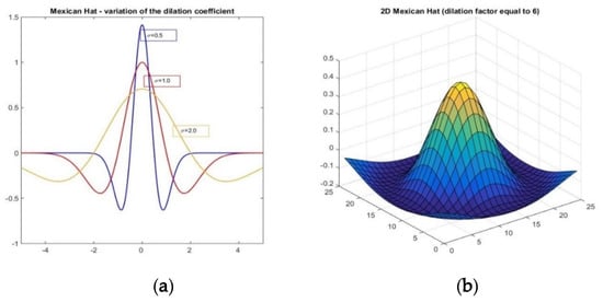
Figure 1.
(a) The dilation coefficient σ and the geometry of the Mexican Hat wavelet for the 1-dimensional case. (b) 3D view of a 2-dimensional Mexican Hat wavelet.
Since we handled discrete signals, we considered discretized versions (e.g., [30]) of the continuous wavelets indicated above. More precisely, for an odd natural number m and for a scaling factor σ, we generated a m × m matrix fm,σ by means of a regular sampling procedure, so that the value at the central cell of the matrix is ψσ (0, 0). Formally, considering rows and columns as corresponding to the y-coordinate and to the x-coordinate, respectively, we defined the filter fm,σ by the formula:
2.2. Study Approach and Software Development
The overall concept of the software tool (available from https://github.com/CeLTIS-UB/WaveletsTool) is described in Figure 2. As indicated in the diagram, the basic input data is a surface/canopy model in raster format. The cell size also needs to be indicated.
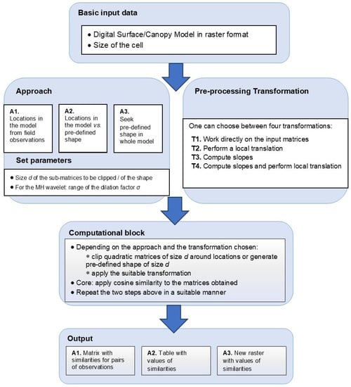
Figure 2.
Concept of the software instrument. The white blocks represent data provided by the user or choices to be made before running the instrument. For each of the three approaches (A1, A2, A3) chosen in the “Approach” block, a suitable output is provided. The pre-processing transformations are coded T1, T2, T3, and T4.
Approaches: use of field observations and pre-defined shapes. For developing the functionalities of the software tool, we took into account the fact that there are two different types of data to deal with in order to perform shape comparisons. The first refers to locations derived from field observations. Specifically, one assumes that field data collected with a GPS device were transferred to the GIS environment, making it possible to indicate the positions of the field observations as cells of the surface/canopy model. In the following, the positions of the observations are called locations in the surface/canopy model (in the study case described later in this paper, these were tree locations). The second type of data is a pre-defined shape generated by a suitable algorithm. The instrument allows choosing between the Mexican Hat wavelet (used throughout the study) described in Section 2.1.2, and a filter customized by the user. For the latter choice, the values of the filters need to be provided in files and they can be uploaded from a local folder. Therefore, we implemented three possible approaches (denoted by A1, A2, A3). These approaches combine the two data sources and represent the potential stages of an entire workflow. Firstly (in approach A1), one handles only locations derived from the field observations for choosing a suitable pre-processing transformation or for comparing the available surface/canopy models of the site. Then (in approach A2), one calibrates the pre-defined geometric shape by measuring its similarity with the true vegetation or landscape patterns available from the field observations. Finally (in approach A3), by using the outcomes of the previous stages, one seeks the occurrence of the pre-defined shape in the entire surface/canopy model.
The choice of the approach is suitably indicated in the graphical user interface and requires setting appropriate parameters. Common to all approaches is the size d of the (sub-)matrices to be compared. For the approaches relying on locations, one has to load a shape file from which the instrument automatically derives the locations in the surface/canopy model. If, in the approaches involving a pre-defined shape, the user chooses to work with the Mexican Hat wavelet, the tool allows a choice for the dilation factor σ from among an entire set of values equidistantly distributed; the minimal and the maximal values, together with the step, have to be filled in in the graphical user interface. We now briefly provide a description of the three approaches.
- The first approach (A1) relies only on locations in the surface/canopy model. It enables pairwise comparisons of sub-matrices centered at cells of the surface/canopy model corresponding to the locations identified in the field. In this case, the output is a square matrix whose entries are the similarities values corresponding to all the pairs of locations.
- The second approach (A2) combines the work with locations in the surface/canopy model and with a pre-defined shape or with a whole family of pre-defined shapes, as described above. It makes it possible to compare sub-matrices of the surface/canopy model corresponding to true terrain shapes with the pre-defined geometric form. The output for this approach is a table with the similarity values; the rows correspond to the locations and the columns correspond to the different shapes considered—the values of the dilation factor σ in the case of the Mexican Hat.
- The third approach (A3) uses only a pre-defined shape besides the surface/canopy model. It seeks to identify the occurrence of the chosen geometric form in the entire surface/canopy model. For a fixed pre-defined shape, the output is a table that corresponds to the similarity values. If one considers a whole family of pre-defined shapes, then the tables are saved separately.
The output can be saved in standard file formats so that it can be used for subsequent analyses. Independent of the approach, the core part is the computation of similarity between matrices, by using the mechanism indicated in Section 2.1.1. As described in Section 2.1.1, there are four options for transforming the matrices in a pre-processing step (the transformations T1, T2, T3, and T4; also see Figure 2). Once chosen for a run session, the methods act on every input matrix. Depending on the choices made by the user, in the computational block of the instrument the appropriate data is selected and suitable computations are performed.
Instrument development. The accompanying software tool was developed in two variants, one in Esri’s ArcGIS Platform as a geoprocessing tool, and the other using only Opensource libraries. We used Python as the scripting language. The instrument’s back-end is common for both versions and uses NumPy, SciPy, and Pandas libraries for the main matrix processing, data handling, and other mathematical computations. The front-end (GUI) part was implemented differently. The GUI for the Esri version depends on the software environment settings of ArcMap or ArcGIS Pro desktop applications. Methods from the ArcPy library were used for the vector data analysis and raster format conversions. This version works in both Python 2 and 3 without the need to perform any script adjustments. The Opensource version of the GUI is built using the Tkinter library and uses GDAL/OGR (Geospatial Data Abstraction Library) for raster conversion and vector data analysis. This version only works for Python 3 and can be easily deployed using the Conda environment created for this purpose. The output differs according to the processing approach chosen but consists of CSV (comma-separated values) tables or raster files.
2.3. Study Area
The study area (Figure 3a) was located in the Fundata commune (Rucăr-Bran Passageway, Romanian Southern Carpathians), Brașov county, at the approximate coordinates 45°25’52” N latitude, 25°15’35” E longitude. The terrain follows a couloir shape with moderate slopes, small limestone outcrops, and altitudes that vary between 1290 m and 1350 m. Tree species present at the site are mostly Norway spruce (Picea abies) and European beech (Fagus sylvatica). The tree height varies between 2 and 20 m. Small bushes of juniper (Juniper communis) with a maximum height of 3m are also present.
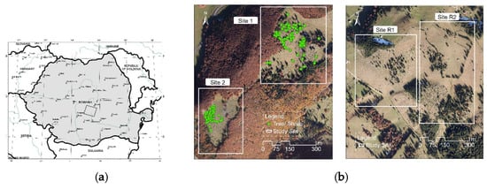
Figure 3.
(a) Location of the study area in the Romanian Carpathians; (b) Orthophotomaps of the four sites selected (left sites 1 and 2, right sites R1 and R2). In sites 1 and 2, the locations of the trees/shrubs identified in the field are represented.
Inside the study area we considered four distinct sites (Figure 3b). The sites had the characteristics of a wood pasture, the vegetation cover being a mixture of grass, shrubs, and groups of trees. The first two sites were labelled as Site 1 (with a surface of 16 ha) and Site 2 (with a surface of 9 ha). We focused on two types of vegetation features, namely, in Site 1, we identified 77 coniferous trees with heights ranging from 1 to 25 m, and in Site 2 we identified 95 juniper shrubs with heights ranging from 0.5 to 3 m. For each tree/shrub we recorded in the field the location, the tree species (coniferous, deciduous, or juniper), and if the tree was singular or clumped together with other trees forming groups. In order to mark the locations of the vegetation features in the field, we used a Garmin 76 GPS device with a 3 m ground accuracy and recorded the locations in a WGS84 coordinate system. We encountered small issues when recording the locations of the trees because we could not place the GPS in a perpendicular direction to the top of the tall trees or some of the juniper ones, so we acquired the locations by placing the GPS device as close as possible to the features, either tangent to the tree trunks or above the juniper shrubs where possible. Acknowledging the GPS error of ±3 m, as a pre-processing step the GPS locations recorded in the field were then corrected manually in ArcGIS. Thus, the top of the trees was set by automatically moving the locations to the maximum local value found in the surface/canopy model. This “move to maximum” pre-processing step was also included in the software tool as an option to automatically correct these general GPS placement errors and to ensure the reproducibility of the research. The third site (with a surface of 16 ha) and the fourth site (with a surface of 20 ha), labelled as Site R1 and Site R2, respectively, were selected for validation. They had a similar vegetation cover, but the pattern was more varied: for instance, one can notice the hedges in the northern half of the site R2. For these sites, no data regarding the location of vegetation features was collected in the field.
2.4. Data
A high-resolution LiDAR point cloud was acquired for a larger surface including the study area, through an aerial survey carried out by the company Primul Meridian in autumn 2013. The data was collected with a Riegl LMS-Q560 scanner, and it was post-processed with the Riegl specific software tools. The company classified the points in the cloud as ground, vegetation, and other classes (e.g., buildings, haystacks, other constructions) by using the TerraScan software. They provided the point cloud, with an average point density of 22.5 points/m2, in the LiDAR Data Exchange Format (LAS) format. We further processed the point cloud using the tools of the ArcGIS 10.1 software. We generated two regular grids both with a cell size equal to 1m: the Digital Surface Model (DSM) and the Canopy Height Model (CHM). The choice of the cell size was made as a trade-off between the original data density and the need to compare the surface/canopy models with a smooth shape (the Mexican Hat wavelet). Thus, the size of the cell was set to be equal to 1m, which is a resolution that suitably defines scattered trees at landscape level, while higher resolutions would have revealed patterns we were not interested in. This choice also matched the range of crown diameter to cell size (between 3:1 and 19:1) suggested in [58]; for the vegetation features in Sites 1 and 2, the ratio was equal to 10:1 and to 3:1, respectively.
The DSM was generated by using the points classified as vegetation. The CHM was derived as the raster difference between the DSM and the terrain model. The latter was generated from the ground points by taking into account the last returns of the LiDAR pulses. For generating the grids, we selected the natural neighbor interpolation method with ground belonging to the DSM [59]. This choice was in line with recent studies [60], proving that this interpolation method yields the most accurate models. Finally, we clipped regular grids corresponding to Sites 1 and 2 from the CHM and the DSM. The GPS point locations of the trees obtained in situ with the GPS device were transferred to the GIS environment and were linked to the geodatabase of the study site.
2.5. Study Design
The study included three stages related to the three approaches (A1, A2, A3) described in Section 2.2., thus combining data collected in situ with the use of pre-defined shapes, namely the Mexican Hat wavelets. We firstly explored the relationship between the pre-processing transformations that can be applied to the data before computing the similarity. Secondly, we investigated to what extent the geometric shape of the Mexican Hat can be considered as a proxy for identifying vegetation features such as isolated trees. Finally, we estimated the potential location of scattered trees by taking advantage of their resemblance to the pre-defined geometric shape.
2.5.1. Exploratory Analysis: Comparisons of the Pre-Processing Transformations and of Surface Versus Canopy Height Models
Computation of similarities: When choosing the approach A1, the output of a run session is represented by a square matrix having, as entries, the similarities between sub-matrices centered at locations in the surface/canopy model used as inputs. In the following, the locations are chosen to correspond to the vegetation features identified in the field. We used the approach A1 for comparing the four pre-processing transformations (T1, …, T4) described in Section 2.1.1 as well as the use of the Canopy Height Model (CHM) versus the use of the Digital Surface Model (DSM). The aim was to understand whether the similarities corresponding to the various choices were correlated or whether any one of the possible choices better reflected the data variability and, consequently, the differences between the shapes of the vegetation features.
Let us first recall that one needs to choose a value d, indicating the dimension of the square sub-matrix clipped from the surface/canopy model around the locations (see Section 2.2 and Figure 2). We considered three values, namely d = 3, d = 5, and d = 7, so that the sub-matrices clipped were compatible with the expected size of the tree (recall that the cell size of the regular grids considered was equal to 1m). For a fixed size d, the choice of a pre-processing transformation and the use of CHM or DSM thus yielded eight possible combinations, coded as CHM_T1, …, CHM_T4 and DSM_T1, …, DSM_T4. For each size and for each of the eight combinations, we separately ran the software tool developed. Since the similarity matrices were symmetric, we retained only their lower parts and we transformed them into vectors. Altogether, for each site and for each size d, we obtained eight vectors of values, corresponding to the eight combinations described above.
Principal Component Analysis: We explored the variability of the data in the vectors of similarities and how the various choices were related to this variability by using standard multi-variate statistics. Specifically, for each site and for each size d, we applied a Principal Component Analysis (PCA) by following the methodology in [61]. The quantitative descriptors (variables) were the eight combinations yielded by the four pre-processing transformations and the choice of the DSM/CHM as the data source. The input data (observations) were the values of the vectors of the similarities previously computed. The goal of the PCA was to reduce the dimensionality of the data and to find new coordinates that were meaningful with respect to the data variability—the principal components. We used suitable functions of the MATLAB scientific software and we determined the variability explained by the new coordinates and the projections of the original descriptors on the principal components (the loadings). For a visual interpretation, we generated biplots with the descriptors, the principal components, and the projections of the objects. As a goodness-of-fit measure, we computed the correlation between (i) the distances between the original objects and (ii) the distances between the projections of the objects in the plane determined by the first two principal components.
2.5.2. Accuracy Assessment
For the second approach A2, we used the pre-defined shape implicitly provided by the instrument, namely the Mexican Hat wavelet (recall that the shape of a Mexican Hat was controlled by the dilation factor σ) and the true vegetation features identified in situ. We followed two tracks: (i) to estimate the best matching dilation factors and (ii) to find a threshold for the similarity values corresponding to the tree locations.
Best matching dilation factor: We considered the vegetation features identified in the field, and for each feature we sought the value of the dilation factor σ yielding the best matching Mexican Hat wavelet. For each site, we ran the software tool by choosing for the dilation factor the range [0.0, 5.0] with steps of 0.01. The maximal value 5.0 was selected after a preliminary assessment of the behavior of the Mexican Hat wavelet and by analyzing the variation in the similarity values for several individual features (Supplementary Material, Figure S1). The choice of a reference model and a suitable pre-processing transformation was made by taking into account the outcomes of the exploratory statistical analyses. We again considered three possible sizes for the matrices to be compared, namely d = 3, 5, 7, which means that we chose m = 3, 5, 7 in Formula (4). Then, for each d and for every vegetation feature (tree/shrub), we selected the best matching dilation factor, which was the value of σ for whichever one obtained a higher similarity value with the matrix clipped around the feature.
Threshold for the similarity values corresponding to tree locations: The natural patterns were not perfectly regular and therefore it was hard to find a perfect similarity between a vegetation feature and a Mexican Hat wavelet. It was therefore natural to seek a threshold value t, so that a similarity above this threshold between a surface/canopy model sub-matrix around a given location and a Mexican Hat wavelet would indicate that the location corresponded to a scattered tree. To find a suitable value of t, we proceeded as follows. We regarded the tree detection as a typical presence/absence problem [62]. In Site 1 and Site 2 (where field observations were available), we considered locations in the surface/canopy model labelled as “trees” and “non-trees”, respectively. The former corresponded to the scattered trees identified in the field. For the latter, we manually mapped locations corresponding to the ground or other features, such as non-isolated trees in a forest. In Site 1, we considered 150 samples of locations (77 trees and 73 non-trees), and in Site 2 we chose 200 samples (95 trees and 105 non-trees). The size d of the window was successively selected to be equal to 3, 5, and 7 for Site 1. For Site 2, the size d was set to be 3 and 5, since in this site the vegetation features (juniper shrubs) had a smaller spatial extent. For each d, we again applied Formula (4) by putting m = d and by selecting the dilation factor σ to range in the interval 0.1–5.0, thus getting similarity values for the chosen locations. For the threshold t, we classified a location as a predicted “tree” if, for any size d, there existed a dilation factor σd so that the similarity value corresponding to σd was greater than or equal to t (heuristically, this meant that each surface/canopy model sub-matrix around the location resembled a certain Mexican Hat wavelet). Otherwise, the location was classified as a predicted “non-tree”. We then compared the actual classification (“tree” versus “non-tree”) to the predicted one. Thus, for each t we assessed the overall accuracy of the detection [63] as the percentage of correctly classified samples (in both categories “tree” and “non-tree”). We also computed two indicators widely used in threshold dependent models, namely the percentage of false positives (Type I errors/commission errors) and false negatives (Type II errors/omission errors).
2.5.3. Similarity Values, Simultaneous Matching and Locations of Potential Trees
In the last step, we illustrated the use of Approach 3 to identify the potential locations of scattered trees or shrubs for the four sites. By taking into account the size of the vegetation features to be identified, the size d of the moving window was successively selected to be equal to 3, 5, and 7 for the sites 1 and R1, while for sites 2 and R2 d was selected to be equal to 3 and 5. For each d, we applied again Formula (4) by putting m = d and by selecting the dilation factor σ to range in the interval 0.0–5.0. For each site and for each choice, we obtained a matrix of similarity values. The cells for which there was a similarity value above the threshold value determined in the previous step were considered to have a value of 1, and the remaining to have a value of 0. Thus, for each d we obtained matrices with ones and zeros. We then selected only the entries with a value of one for all sizes, indicating a simultaneous matching. Finally, for each site we obtained a matrix of ones and zeros with the same size as the surface/canopy model, the ones indicating a potential location of a vegetation feature (tree or shrub).
3. Results
We now illustrate the use of the software tool in a study case, based on the data described in Section 2.3. We considered the three approaches described in the methodology (approaches A1, A2, A3), thus combining data collected in situ with the use of pre-defined shapes, namely the Mexican Hat wavelets.
3.1. How Do the Pre-Processing Transformations Influence the Outcomes?
According to the study design described in Section 2.5, we first computed the similarities for sub-matrices clipped around the field locations and applied a Principal Component Analysis for understanding the influence of various choices. The cumulated data variability explained by the first two components for d = 3, 5, 7 was approximately 88.52%, 74.32%, and 73.77% respectively for Site 1 and 87.58%, 77.64%, and 75.23% respectively for Site 2 (see Table 1 and Table 2). On the other hand, except for one case, the percentage of the explained variability corresponding to the third component was less than the threshold value of 15.22% [64]. The distances between the original objects and their projections in the plane generated by the first two components were well correlated. For Site 1, the values of the chosen goodness-of-fit measure were equal to 0.9877 (d = 3), 0.9222 (d = 5), and 0.9246 (d = 7), and for Site 2, the values were equal to 0.9819 (d = 3), 0.9543 (d = 5), and 0.9603 (d = 7). Therefore, one might conclude that the first two components are relevant for assessing the data variability, and that it is meaningful to interpret the original descriptors with respect to the new axes.

Table 1.
Data variability explained by the first three principal components (PC1, PC2 and PC3) for Site 1.
Table 2.
Data variability explained by the first three principal components (PC1, PC2 and PC3) for Site 2.
The values of the loadings for all the descriptors can be found in Table 3 and Table 4, and the corresponding biplots are represented in Figure 4. Visually, the arrows corresponding to the transformation T3 are better aligned with the first principal axis. Indeed, in almost all cases (five out of six), DSM_T3 had the longest projection on the first component. This result hints that by applying the transformation T3 (namely, computing slopes towards the center), one better captures the variability of the vegetation features considered. We also notice that for d = 5 and d = 7, the arrow associated with transformation T4 is better correlated to the second principal component. Let us recall the interpretation of the transformations T3 and T4 and their relationship to the z-values’ variation in first order and second order, which in turn could be related to indicators such as slopes and curvatures, respectively (e.g. [65]). Thus, we might conclude that such indicators are relevant for explaining the variability of the tree shapes.
Table 3.
Projections of the first principal components and the length of the projections for Site 1.
Table 4.
Projections of the first principal components and the length of the projections for Site 2.
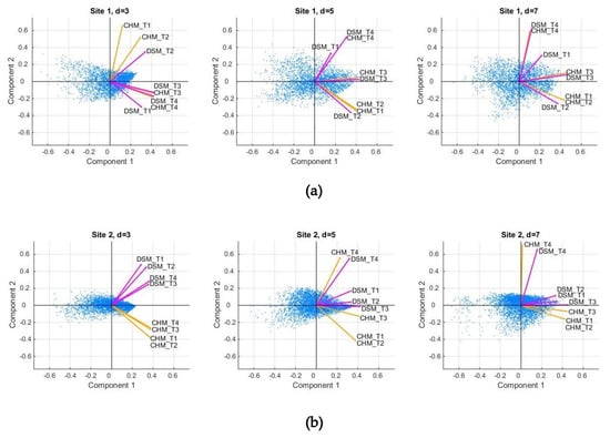
Figure 4.
Results of the Principal Component Analysis. The row (a) corresponds to Site 1 and the row (b) to Site 2. The codes of the descriptors are obtained from the eight possible choices: four pre-processing transformations (T1, T2, T3, and T4) and two types of models (Canopy Height Model (CHM)—orange arrows; Digital Surface Model (DSM)—magenta arrows).
The direct use of the z-values (i.e., the application of the identity transformation T1) may impact the computed similarity. This can be observed in Figure 4, where T1 (relying directly on the z-values) provides weak correlations for the values obtained when working on the CHM compared to the ones obtained for the DSM. The other methods have better correlations for the two data sources since, before computing the cosine similarity, a (local) transformation is performed, thus eliminating the impact of the absolute value.
In the following, we briefly describe a synthetic example, emphasizing the role played by the values compared to the effective shape of the matrices compared. We consider a 3 × 3 matrix representing a tree selected from Site 1, and we generate an arbitrary shape that hardly resembles a tree (e.g., the central value is a local minimum, while for a tree it is expected to be a local maximum).
.
However, the cosine similarity as obtained without performing any transformation is rather high (equal to 0.98). Let us notice that, by applying the transformations T2, T3, and T4, the values obtained are equal to 0.62, −0.87, and 0.57, respectively, and they clearly hint at a weak similarity between the tree and the synthetic shape.
In a nutshell, we concluded that the first step enabled us to perform comparisons between various transformations could be applied before computing the similarity. For the study case handled in the analyses, we found that working on the DSM and performing the transformation T3, corresponding to the z-values variation, better reflected the variability of the vegetation features.
3.2. To What Extent Do Trees Resemble Mexican Hat Wavelets?
According to the study design, we took into account the comparative analyses between the pre-processing transformations. We applied the transformation T3 before the comparison of the similarity values and chose the DSM as a reference model. The medians of the best matching values for Site 1 were equal to 0.97, 1.39, and 1.53 for the three selected cell sizes, d = 3, 5, 7, respectively. For the second site, these values were 0.77, 0.47, and 0.26, respectively (see Supplementary Material, Tables S1 and S2). In Figure 5, we represented in box plots the quartiles corresponding to the best matching dilation factors for the two sites. Both from the median values and the graphical representation, one can deduce that there is a slight difference between the best matching dilation factors corresponding to the coniferous trees and the ones corresponding to the juniper shrubs, which could be due to the different 3D shapes of the vegetation features.
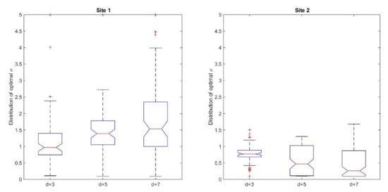
Figure 5.
Box plots of the best matching dilation factors σ corresponding to the vegetation features selected in the two sites.
These outcomes could be put in a relationship with the geometry of the Mexican Hat wavelet (Figure 1), as induced by the dilation factor σ; for smaller values of σ, the peak of the graph is higher, while the curve is sharper around the center and becomes quickly flat. This difference can be seen when comparing the behavior of the best matching values for the two sites when the size of the cell increases. Thus, for the site with coniferous trees, the median best matching value and the values defining the quartiles have a slight increase, while for the site with juniper shrubs, the opposite happens. This behavior could be explained by the different geometric shapes of the shrubs; the contour of the vegetation feature indicates a steep decrease around the center combined with flatness towards the borders of the clipped sub-matrix. On the other hand, shapes in nature are not necessarily regular, therefore artefacts might occur. For instance, some of the trees have an asymmetric shape due to natural variation or local environmental factors, are clumped together in small groups, or have intertwined canopies; this can be reflected by the z-values in the grid. As shown in Figure 6a on the CHM and Figure 6b on the ortophotomap, some isolated trees can form small individual groups that present a pronounced asymmetry regarding their shape. Other than that, inherent errors due to the measurements or to the interpolation process that transformed the point cloud into a regular grid could lead to such asymmetries. Despite the irregularities, we might conclude that the distribution of the best matching dilation factors reflects the different vegetation features identified in the two sites.
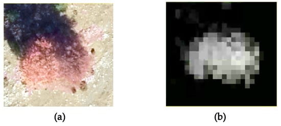
Figure 6.
Example of tree shape asymmetry in the ortophotomap (a) and CHM (b).
Threshold for similarity values corresponding to tree locations: The graphical representation (Figure 7) hints that in the case of Site 1, the best prediction is obtained for the threshold value t = 0.7, with an overall accuracy of 88.7%, an omission error of 11.3%, and no commission error. For Site 2, the best overall accuracy is equal to 77.5%, and it is obtained for the threshold values 0.65 and 0.7. We chose the former, since the percentage of true positives is 42.5%, compared to 39.5% for the latter. For this threshold value, the omission error is 5% and the commission error is 17.5%. The confusion matrices corresponding to the selected threshold values can be found in Table 5 and Table 6. Summing up, the threshold values 0.7 (for Site 1) and 0.65 (for Site 2) were chosen as reference values for comparing locations in the surface/canopy models with the pre-defined geometric shapes considered in the study.
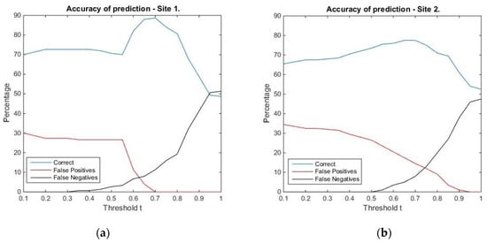
Figure 7.
Accuracy of the prediction for the locations in Site 1 (a) and Site 2 (b). The percentage of correctly classified locations of false positives and false negatives were computed for values of the threshold t running between 0.1 and 1 with steps of 0.05.
Table 5.
Confusion matrix (counts) for 150 locations (labelled as “tree” and “non-tree”) in Site 1. The actual classification is compared to the classification predicted by choosing a threshold for the similarity value equal to 0.7.
Table 6.
Confusion matrix (counts) for 200 locations (labelled as “tree” and “non-tree”) in Site 2. The actual classification is compared to the classification predicted by choosing a threshold for the similarity value equal to 0.65.
3.3. How Can One Determine the Locations of Scattered Trees?
Several choices were necessary in the last stage, and they were determined by the outcomes of the previous steps. Thus, we chose the pre-processing transformation T3 (corresponding to the slopes) and the DSM as the data source, as indicated by the findings in Section 3.1. The threshold value indicating a potential location of a tree was set at 0.7 for Sites 1 and R1, and it was set at 0.65 for Sites 2 and R2, as indicated by the analyses in Section 3.2.
For the sites 1, 2, R1, and R2, we found 1079, 2723, 1107, and 5331 potential tree locations, respectively. Let us notice that, for Site 1, out of 77 trees identified in the field, 60 were indicated as potential tree locations, which yields an accuracy of 77.9%. For Site 2, out of 95 shrubs, 85 were found as potential locations (accuracy of 89.5%).
For visualization purposes, we transformed the matrices into rasters and then into shape files by using the suitable tools of the ArcGIS 10.1 software. An overlay with the orthophotomaps provided the spatial distribution of the potential locations (Figure 8). One can notice that, visually, the outcomes are very plausible. For instance, in sites 1 and 2 most of them are situated in the middle part, namely in the pasture, where scattered trees can be indeed found in situ. In Site 1, few potential tree locations were indicated in the denser forests, hinting that the surface/canopy model around a scattered tree is different to the surface/canopy model around a tree situated in a forest. In Site R2, the trees belonging to the hedge situated in the northern half were identified as potential locations. The slight mismatch between the tree labels and the image could be due to the different spatial resolutions (the orthophotomap had a resolution of 12 cm, while the surface/canopy model had a resolution of 1 m).
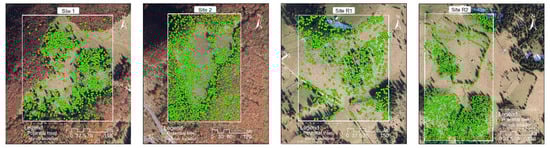
Figure 8.
Potential locations of scattered trees labelled on the orthophotomaps.
In the Supplementary Material, we included in Figure S2 an application for two other sites with different characteristics. The outcomes are similar and confirm that the proposed approach could be successfully used in various environments.
4. Discussion
In summary, we might conclude that choosing suitable dilation factors for the Mexican Hat wavelet makes it possible to find potential locations for scattered trees or shrubs. Furthermore, as a subsequent step, one can extract from the canopy height model or the digital surface model an estimate of the tree heights. This is a general advantage of an approach relying on the vertical structure of the vegetation when compared to ones based only on two-dimensional imagery (even high-resolution).
Let us notice that, for Site 1, out of 77 trees identified in the field, 60 were indicated as potential tree locations, which yields an accuracy of 77.9%. For Site 2, out of 95 shrubs, 85 were found as potential locations (accuracy of 89.5%). Similar studies, which aimed to detect trees in remote sensing data, reported similar results. In [17], six crown detection algorithms were investigated using aerial images under various forest conditions. The best accuracies reported varied from 60% for dense forest with a region growing algorithm to 99.7% for plantation with a marked point process algorithm. However, the authors warn that the algorithms are over-adapted for the specific forest type. Studies using data derived from LiDAR or Unmanned Aerial Vehicles (UAV) cite slightly higher accuracies ranging from 80% to 90% [9,18,66,67,68,69], while recent deep learning developments reached accuracies of >90% [4,70,71].
LiDAR and other remote sensing data can be used to detect vegetation patterns at different scales, from small plants [72,73] to whole forests [74]. It is important to note that the results are not immediately comparable between studies due to different data sets, pre-processing methods, environmental conditions (natural landscapes, urban areas, tree plantations), and not least, object detection techniques [75]. Our method has the advantage that it is not bound to specific pre-processing tasks on LiDAR data. It works on any 2D matrix of elevation data, irrespective of the original source data, as we showed with the results on the CHM and DSM models. Also, unlike other tree detection methods in which model training is resource intensive and time consuming, the method we presented does not require such steps. Furthermore, the software tool contributes greatly to the reproducibility of the method, as it allows the user to easily follow the processing steps shown without the need to worry about implementing complex mathematical processing on matrix data. There is also a high degree of versatility to the tool and the described method, as it supports the detection of various shapes by simply using another wavelet filter or a generic 2D filter which describes the shape to be detected.
We illustrated the approach proposed and the functionalities of the software tool for solving a specific problem (the detection of scattered trees). However, the whole approach as well as the software instrument were conceived as a tool to be used in various analyses relying on regularly gridded surface/canopy models. Therefore, it offers the user the freedom to choose several approaches and parameters, providing appropriate outputs. Moreover, one could design, implement, and test alternative geometric shapes, depending on the problem under investigation. Thus, further possible applications refer to the comparison/detection of other vegetation patterns, geomorphologic features, or whole 3D landscape patterns.
5. Conclusions
The problem investigated in this paper was the detection of scattered trees in high resolution surface/canopy models. For achieving this aim, we developed and presented an approach and an accompanying software tool whose functionalities enable the comparison or the identification of landscape/vegetation patterns.
We proposed to address the issue by emphasizing the role of the 3D geometry of the objects of interest. Therefore, we explored the variability of regularly gridded digital surface/canopy models, regarded as discrete 2D signals. Thus, we adapted techniques stemming from pattern detection and we applied the cosine similarity measure to matrices whose entries were related to the vertical structure. We found that, when using surface/canopy models, the shape variability was better assessed by applying a pre-processing transformation based on slopes computation, corresponding to the variation in first order of the z-values.
In this paper, we presented an entire workflow that made it possible to find potential locations of scattered trees or shrubs from a digital surface model. This was achieved by using a pre-defined shape as a geometric model, the Mexican Hat wavelet resembling a coniferous tree. For two study sites, the trees and shrubs that were previously identified in the field were detected by our approach with accuracy rates of 77.9% and 89.5%. Moreover, in both sites and in four other sites with different characteristics chosen for validation, a visual check based on orthophotomaps confirmed the reliability of the outcomes.
6. Patents
There is no patent resulting from the work reported in this manuscript.
Supplementary Materials
The following are available online at https://www.mdpi.com/2220-9964/9/5/298/s1. Figure S1: Plots of similarity values for three trees from Site 1 (row above) and three juniper shrubs from Site 2 (row below). The dilation factor ranges from 0.0 to 5.0 and the size of the matrices compared is d = 3, 5, 7. Figure S2: Potential locations of scattered trees labelled on orthophotomaps for two replicate sites in Germany. Row above: site Friedrichroda; row below: site Luisenthal. Since no obvious pattern of scattered trees was identified in the examples, we included a zoom area for each site in order to show how the detected locations match the ground truth data. The LiDAR point cloud data and the high resolution RGB imagery were obtained from the Thuringian State Office for Soil Management and Geographic Information (Thüringer Landesamt für Bodenmanagement und Geoinformation). The geoportal (https://www.geoportal-th.de/de-de/, accessed on 27 March 2020) allows the user to download pre-processed LiDAR datasets as point clouds to directly derive the Digital Surface Model (DSM) through interpolation, without the need of other processing steps. We used ArcGIS Pro software to generate the DSM model from the LiDAR data at 1m spatial resolution. Table S1: quantiles for the optimal dilation factor σ for Site 1. Table S2: quantiles for optimal dilation factor σ for Site 2.
Author Contributions
Conceptualization, Mihai-Sorin Stupariu; methodology, Mihai-Sorin Stupariu, Alin-Ionuț Pleșoianu; validation, Ileana Pătru-Stupariu, Christine Fürst; investigation, Mihai-Sorin Stupariu, Alin-Ionuț Pleșoianu, Ileana Pătru-Stupariu; software development Mihai-Sorin Stupariu, Alin-Ionuț Pleșoianu; writing—original draft preparation, Mihai-Sorin Stupariu, Alin-Ionuț Pleșoianu; writing—review and editing, Ileana Pătru-Stupariu, Christine Fürst; supervision, Ileana Pătru-Stupariu, Christine Fürst. All authors have read and agreed to the published version of the manuscript.
Funding
The data used in the study were acquired in the project WindLand, project code: IZERZO 142168/1 (funded by SNSF) and 22 RO-CH/RSRP (funded by UEFISCDI), developed within the framework of the Romanian–Swiss Research Programme. Alin-Ionuț Pleșoianu acknowledges the financial support received from the Doctoral School Simion Mehedinti, Faculty of Geography, University of Bucharest.
Acknowledgments
Mihai-Sorin Stupariu and Ileana Pătru-Stupariu acknowledge the support and the stages provided by the Martin-Luther-Universität Halle-Wittenberg. We would also like to thank www.RonningTranslation.com for their professional copy-editing of a preliminary version and Mrs. Luminița Olteanu for a careful check and proofing of the final version. We also thank the reviewers for their constructive comments and suggestions.
Conflicts of Interest
The authors declare no conflict of interest. The funders had no role in the design of the study; in the collection, analysis, or interpretation of data; in the writing of the manuscript; or in the decision to publish the results.
References
- Walz, U.; Hoechstetter, S.; Dragut, L.; Blaschke, T. Integrating time and the third spatial dimension in landscape structure analysis. Landsc. Res. 2016, 41, 279–293. [Google Scholar] [CrossRef]
- Morelli, F.; Benedetti, Y.; Simova, P. Landscape metrics as indicators of avian diversity and community measures. Ecol. Ind. 2018, 90, 132–141. [Google Scholar] [CrossRef]
- Chakraborty, A.; Sachdeva, K.; Joshi, P.K. A reflection on image classification for forest ecology management: Towards landscape mapping and monitoring. In Handbook of Neural Computation; Samui, P., Roy, S.S., Balas, V.E., Eds.; Academic Press—Elsevier Science: London, UK, 2017; pp. 67–85. [Google Scholar]
- Li, W.; Dong, R.; Fu, H.; Lee, Y. Large-Scale Oil Palm Tree Detection from High-Resolution Satellite Images Using Two-Stage Convolutional Neural Networks. Remote Sens. 2019, 11, 11. [Google Scholar] [CrossRef]
- Popescu, S.C.; Wynne, R.H.; Scrivani, J.A. Fusion of small-footprint lidar and multispectral data to estimate plot-level volume and biomass in deciduous and pine forests in Virginia, USA. Forest Sci. 2004, 51, 551–565. [Google Scholar]
- Ghosh, A.; Fassnacht, F.E.; Joshi, P.K.; Koch, B. A framework for mapping tree species combining hyperspectral and LiDAR data: Role of selected classifiers and sensor across three spatial scales. Int. J. Appl. Earth Obs. Geoinf. 2014, 26, 49–63. [Google Scholar] [CrossRef]
- Evans, J.S.; Hudak, A.T. A Multiscale Curvature Algorithm for Classifying Discrete Return LiDAR in Forested Environments. IEEE Trans. Geosci. Remote 2007, 45, 1029–1038. [Google Scholar] [CrossRef]
- Dubayah, R.; Drake, J. Lidar remote sensing for forestry. J. Forest 2000, 98, 44–46. [Google Scholar]
- Guerra-Hernández, J.; Cosenza, D.N.; Rodriguez, L.; Silva, C.E.; Tomé, M.; Díaz-Varela, M.; González-Ferreiro, E. Comparison of ALS- and UAV(SfM)-derived high-density point clouds for individual tree detection in Eucalyptus plantations. Int. J. Remote Sens. 2018, 39, 5211–5235. [Google Scholar] [CrossRef]
- Popescu, S.C.; Wynne, R.H.; Nelson, R.F. Estimating plot-level tree heights with lidar: Local filtering with a canopy-height based variable window size. Comput. Electron. Agric. 2002, 37, 71–95. [Google Scholar] [CrossRef]
- Unger, D.R.; Hung, I.K.; Brooks, R.; Williams, H. Estimating number of trees, tree height and crown width using Lidar data. GISci. Remote Sens. 2014, 51, 227–238. [Google Scholar] [CrossRef]
- Hadas, E.; Borkowski, A.; Estornell, J.; Tymkow, P. Automatic estimation of olive tree dendrometric parameters based on airborne laser scanning data using alpha-shape and principal component analysis. GISci. Remote Sens. 2017, 54, 898–917. [Google Scholar] [CrossRef]
- Manzanera, J.A.; Garcia-Abril, A.; Pascual, C.; Tejera, R.; Martin-Fernandez, S.; Tokola, T.; Valbuena, R. Fusion of airborne LiDAR and multispectral sensors reveals synergic capabilities in forest structure characterization. GISci. Remote Sens. 2016, 53, 723–738. [Google Scholar] [CrossRef]
- Guo, X.; Coops, N.C.; Tompalski, P.; Nielsen, S.E.; Bater, C.W.; Stadt, J.J. Regional mapping of vegetation structure for biodiversity monitoring using airborne lidar data. Ecol. Inform. 2017, 38, 50–61. [Google Scholar] [CrossRef]
- Fang, F.; Im, J.; Lee, J.; Kim, K. An improved tree crown delineation method based on live crown ratios from airborne LiDAR data. GISci. Remote Sens. 2016, 53, 402–419. [Google Scholar] [CrossRef]
- Wu, B.; Yu, B.; Wu, Q.; Huang, Y.; Chen, Z.; Wu, J. Individual tree crown delineation using localized contour tree method and airborne LiDAR data in coniferous forests. Int. J. Appl. Earth Obs. Geoinf. 2016, 52, 82–94. [Google Scholar] [CrossRef]
- Larsen, M.; Eriksson, M.; Descombes, X.; Perrin, G.; Brandtberg, T.; Gougeon, F.A. Comparison of six individual tree crown detection algorithms evaluated under varying forest conditions. Int. J. Remote Sens. 2011, 32, 5827–5852. [Google Scholar] [CrossRef]
- Vauhkonen, J.; Ene, L.; Gupta, S.; Heinzel, J.; Holmgren, J.; Pitkänen, J.; Maltamo, M. Comparative testing of single-tree detection algorithms under different types of forest. Forestry 2012, 85, 27–40. [Google Scholar] [CrossRef]
- Wu, J. Effects of changing scale on landscape pattern analysis: Scaling relations. Landsc. Ecol. 2004, 19, 125–138. [Google Scholar] [CrossRef]
- Manning, A.D.; Fischer, J.; Lindenmayer, D.B. Scattered trees are keystone structures—Implications for conservation. Biol. Conserv. 2006, 132, 311–321. [Google Scholar] [CrossRef]
- Peringer, A.; Schulze, K.A.; Stupariu, I.; Stupariu, M.S.; Rosenthal, G.; Buttler, A.; Gillet, F. Multi-scale feedbacks between tree regeneration traits and herbivore behaviour explain the structure of pasture-woodland mosaics. Landsc. Ecol. 2016, 31, 913–927. [Google Scholar] [CrossRef]
- Manning, A.D.; Gibbons, P.; Lindenmayer, D.B. Scattered trees: A complementary strategy for facilitating adaptive responses to climate change in modified landscapes? J. Appl. Ecol. 2009, 46, 915–919. [Google Scholar] [CrossRef]
- Falkowski, M.J.; Evans, J.S.; Martinuzzi, S.; Gessler, P.E.; Hudak, A.T. Characterizing forest succession with lidar data: An evaluation for the Inland Northwest, USA. Remote Sens. Environ. 2009, 113, 946–956. [Google Scholar] [CrossRef]
- Cadavid-Florez, L.; Laborde, J.; Mclean, D.J. Isolated trees and small woody patches greatly contribute to connectivity in highly fragmented tropical landscapes. Landsc. Urban. Plan. 2020, 196. [Google Scholar] [CrossRef]
- Hartel, T.; Hanspach, J.; Moga, C.I.; Holban, L.; Szapanyos, Á.; Tamás, R.; Hováth, C.; Réti, K.O. Abundance of large old trees in wood-pastures of Transylvania (Romania). Sci. Total Environ. 2018, 613–614, 263–270. [Google Scholar] [CrossRef] [PubMed]
- Stoicescu, I.; Pătru-Stupariu, I.; Hossu, C.A.; Peringer, A. Land Use Guidelines to Maintain Habitat Diversity of WoodPastures in the Southern Carpathians Under Projected Climate Change. Landsc. Online 2019, 74, 1–24. [Google Scholar] [CrossRef]
- Casalegno, S.; Anderson, K.; Cox, D.T.C.; Hancock, S.; Gaston, K.J. Ecological connectivity in the three-dimensional urban green volume using waveform airborne lidar. Sci. Rep. 2017, 7, 45571. [Google Scholar] [CrossRef]
- Mallat, S. A theory for multiresolution signal decomposition: The wavelet representation. Pattern Analysis and Machine Intelligence. IEEE Trans. Pattern Anal. Mach. Intell. 1989, 11, 674–693. [Google Scholar] [CrossRef]
- Vetterli, M.; Kovacevic, J.; Goyal, V. Foundations of Signal. Processing; Cambridge University Press: Cambridge, UK, 2014. [Google Scholar]
- Addison, P. Wavelet transforms and the ECG: A review. Physiol. Meas. 2005, 26, 155–199. [Google Scholar] [CrossRef]
- Cho, E.; Chon, T. Application of wavelet analysis to ecological data. Ecol. Inform. 2006, 1, 229–233. [Google Scholar] [CrossRef]
- Schröder, B.; Seppelt, R. Analysis of pattern process interactions based on landscape models—Overview, general concepts, and methodological issues. Ecol. Model. 2006, 199, 505–516. [Google Scholar] [CrossRef]
- Csilla, F.; Sándor, K. Wavelets, boundaries, and the spatial analysis of landscape pattern. Ecoscience 2002, 9, 177–190. [Google Scholar] [CrossRef]
- Dale, M.; Mah, M. The use of wavelets for spatial pattern analysis in ecology. J. Veg. Sci. 1998, 9, 805–814. [Google Scholar] [CrossRef]
- Mi, X.; Ren, H.; Ouyang, Z.; Wei, W.; Ma, K. The use of the Mexican hat and the Morlet wavelets for detection of ecological patterns. Plant. Ecol. 2005, 179, 1–19. [Google Scholar] [CrossRef]
- Ye, X.; Wang, T.; Skidmore, A.K.; Fortin, D.; Bastille-Rousseau, G.; Parrott, L. A wavelet-based approach to evaluate the roles of structural and functional landscape heterogeneity in animal space use at multiple scales. Ecography 2015, 38, 740–750. [Google Scholar] [CrossRef]
- Carl, G.; Kühn, I. Analyzing spatial ecological data using linear regression and wavelet analysis. Stoch. Environ. Res. Risk Assess. 2008, 22, 315–324. [Google Scholar] [CrossRef]
- Cazelles, B.; Cazelles, K.; Chavez, M. Wavelet analysis in ecology and epidemiology: Impact of statistical tests. J. R. Soc. Interface 2014, 11, 20130585. [Google Scholar] [CrossRef]
- Garrity, S.R.; Meyer, K.; Maurer, K.D.; Hardiman, B.; Bohrer, G. Estimating plot-level tree structure in a deciduous forest by combining allometric equations, spatial wavelet analysis and airborne LiDAR. Remote Sens. Lett. 2012, 3, 443–451. [Google Scholar] [CrossRef]
- Cazelles, B.; Chavez, M.; Berteaux, D.; Menard, F.; Vik, J.O.; Jenouvrier, S.; Stenseth, N.C. Wavelet analysis of ecological time series. Oecologia 2008, 156, 287–304. [Google Scholar] [CrossRef]
- Dong, X.; Nyren, P.; Patton, B.; Nyren, A.; Richardson, J.; Maresca, T. Wavelets for agriculture and biology: A tutorial with applications and outlook. Bioscience 2008, 58, 445–453. [Google Scholar] [CrossRef]
- Polansky, L.; Wittemyer, G.; Cross, P.C.; Tambling, C.J.; Getz, W.M. From moonlight to movement and synchronized randomness: Fourier and wavelet analyses of animal location time series data. Ecology 2010, 91, 1506–1518. [Google Scholar] [CrossRef]
- Acerbi-Junior, F.; Clevers, J.; Schaepman, M. The assessment of multi-sensor image fusion using wavelet transforms for mapping the Brazilian savanna. Int. J. Appl. Earth Obs. Geoinf. 2006, 8, 278–288. [Google Scholar] [CrossRef]
- Cheng, T.; Rivard, B.; Sánchez-Azofeifa, A. Spectroscopic determination of leaf water content using continuous wavelet analysis. Remote Sens. Environ. 2011, 115, 659–670. [Google Scholar] [CrossRef]
- Martínez, B.; Amparo Gilabert, M. Vegetation dynamics from NDVI time series analysis using the wavelet transform. Remote Sens. Environ. 2009, 113, 1823–1842. [Google Scholar] [CrossRef]
- Prokoph, A.; Patterson, R. Application of wavelet and regression analysis in assessing temporal and geographic climate variability: Eastern Ontario, Canada as a case study. Atmos. Ocean 2004, 42, 201–212. [Google Scholar] [CrossRef]
- Bradshaw, G.; Spies, T. Characterizing canopy gap structure in forests using wavelet analysis. J. Ecol. 1992, 80, 205–215. [Google Scholar] [CrossRef]
- Shekede, M.; Murwira, A.; Masocha, M. Wavelet-based detection of bush encroachment in a savanna using multi-temporal aerial photographs and satellite imagery. Int. J. Appl. Earth Obs. Geoinf. 2015, 35, 209–216. [Google Scholar] [CrossRef]
- Abd Rahman, M.; Gorte, B. Individual tree detection based on densities of high points of high resolution airborne LiDAR. In GEOBIA 2008: Pixels, Objects, Intelligence GEOgraphic Object Based Image Analysis for the 21st Century; Hay, G.J., Blaschke, T., Marceau, D., Eds.; International Society for Photogrammetry and Remote Sensing: Calgary, AB, Canada, 2008. [Google Scholar]
- Falkowski, M.; Smith, J.A.; Hudak, A.; Gessler, P.; Vierling, L.; Crookston, N. Automated estimation of individual conifer tree height and crown diameter via two-dimensional spatial wavelet analysis of lidar data. Can. J. Remote Sens. 2006, 32, 153–161. [Google Scholar] [CrossRef]
- Strand, E.; Smith, A.; Bunting, S.C.; Vierling, L.; Hann, D.; Gessler, P. Wavelet estimation of plant spatial patterns in multitemporal aerial photography. Int. J. Remote Sens. 2006, 27, 2049–2054. [Google Scholar] [CrossRef]
- Marschner, S.; Shirley, P. Fundamentals of Computer Graphics, 4th ed.; CRC Press, Taylor & Francis Group: Boca Raton, FL, USA, 2015. [Google Scholar]
- Cha, S. Comprehensive survey on distance/similarity measures between probability density functions. Int. J. Math. Mod. Meth. Appl. S 2007, 1, 300–307. [Google Scholar]
- Daubechies, I. Orthonormal bases of compactly supported wavelets. Commun. Pure Appl. Math. 1988, 41, 909–996. [Google Scholar] [CrossRef]
- Kumar, P.; Foufoula-Georgiou, E. Wavelet analysis for geophysical application. Rev. Geophys. 1997, 35, 385–412. [Google Scholar] [CrossRef]
- Rioul, O.; Duhamel, P. Fast algorithms for discrete and continuous wavelet transforms. IEEE Trans. Inform. Theory 1992, 38, 569–586. [Google Scholar] [CrossRef]
- Addison, P. The Illustrated Wavelet Transform. Handbook; Institute of Physics Publishing, The Institute of Physics: London, UK, 2002. [Google Scholar]
- Pouliot, D.A.; King, D.J.; Bell, F.W.; Pitt, D.G. Automated tree crown detection and delineation in high-resolution digital camera imagery of coniferous forest regeneration. Remote Sens. Environ. 2002, 82, 322–334. [Google Scholar] [CrossRef]
- Fang, J.; Peringer, A.; Stupariu, M.S.; Pătru-Stupariu, I.; Buttler, A.; Golay, F.; Porté-Agel, F. Shifts in wind energy potential following land-use driven vegetation dynamics in complex terrain. Sci. Total Environ. 2018, 639, 374–384. [Google Scholar] [CrossRef] [PubMed]
- Szabó, Z.; Tóth, C.A.; Holb, I.; Szabó, S. Aerial Laser Scanning Data as a Source of Terrain Modeling in a Fluvial Environment: Biasing Factors of Terrain Height Accuracy. Sensors 2020, 20, 2063. [Google Scholar] [CrossRef]
- Legendre, P.; Legendre, L. Numerical Ecology, 2nd ed.; Elsevier Science: New York, NY, USA, 1999. [Google Scholar]
- Fielding, A.; Bell, J. A review of methods for the assessment of prediction errors in conservation presence/absence models. Environ. Conserv. 1997, 24, 38–49. [Google Scholar] [CrossRef]
- Story, M.; Congalton, R. Accuracy Assessment: A User’s Perspective. Photogramm. Eng. Remote Sens. 1986, 52, 397–399. [Google Scholar]
- Frontier, S. Étude de la décroissance des valeurs propres dans une analyse en composantes principales: Comparaison avec le modèle du baton brisé. J. Exp. Mar. Biol. Ecol. 1976, 25, 67–75. [Google Scholar] [CrossRef]
- Young, M.; Evans, I. Statistical Characterization of Altitude Matrices; Durham: Report No. 5, Grant DA-ERO-591-73-G0040; Dept. of Geography, University of Durham: Durham, UK, 1978. [Google Scholar]
- Yao, W.; Krull, J.; Krzystek, P.; Heurich, M. Sensitivity analysis of 3D individual tree detection from LiDAR point clouds of temperate forests. Forests 2014, 5, 1122–1142. [Google Scholar] [CrossRef]
- Koma, Z.; Koenig, K.; Höfle, B. Urban tree classification using full-waveform airborne laser scanning. ISPRS Ann. Photogramm. Remote Sens. Spatial Inf. Sci. 2016, 3, 185–192. [Google Scholar] [CrossRef]
- Mohan, M.; Silva, C.A.; Klauberg, C.; Jat, P.; Catts, G.; Cardil, A.; Hudak, A.T.; Dia, M. Individual tree detection from unmanned aerial vehicle (UAV) derived canopy height model in an open canopy mixed conifer forest. Forests 2017, 8, 340. [Google Scholar] [CrossRef]
- Burai, P.; Beko, L.; Lenart, C.; Tomor, T.; Kovacs, Z. Individual Tree Species Classification Using Airborne Hyperspectral Imagery and Lidar Data. In Proceedings of the 2019 10th Workshop on Hyperspectral Imaging and Signal Processing: Evolution in Remote Sensing (WHISPERS), Amsterdam, The Netherlands, 24–26 September 2019; pp. 1–4. [Google Scholar]
- Tianyang, D.; Jian, Z.; Sibin, G.; Ying, S.; Jing, F. Single-Tree Detection in High-Resolution Remote-Sensing Images Based on a Cascade Neural Network. ISPRS Int. J. Geo-Inf. 2018, 7, 367. [Google Scholar] [CrossRef]
- Freudenberg, M.; Nölke, N.; Agostini, A.; Urban, K.; Wörgötter, F.; Kleinn, C. Large scale palm tree detection in high resolution satellite images using U-Net. Remote Sens. 2019, 11, 312. [Google Scholar] [CrossRef]
- Zlinszky, A.; Molnár, B.; Barfod, A.S. Not all trees sleep the same—High temporal resolution terrestrial laser scanning shows differences in nocturnal plant movement. Front. Plant Sci. 2017, 8, 1814. [Google Scholar] [CrossRef]
- Zlinszky, A.; Barfod, A. Short interval overnight laser scanning suggests sub-circadian periodicity of tree turgor. Plant Signal. Behav. 2018, 13, e1439655. [Google Scholar] [CrossRef]
- Simard, M.; Pinto, N.; Fisher, J.B.; Baccini, A. Mapping forest canopy height globally with spaceborne lidar. J. Geophys. Res. Biogeosci. 2011, 116. [Google Scholar] [CrossRef]
- Zhen, Z.; Quackenbush, L.J.; Zhang, L. Trends in automatic individual tree crown detection and delineation-evolution of LiDAR data. Remote Sens. 2016, 8, 333. [Google Scholar] [CrossRef]
© 2020 by the authors. Licensee MDPI, Basel, Switzerland. This article is an open access article distributed under the terms and conditions of the Creative Commons Attribution (CC BY) license (http://creativecommons.org/licenses/by/4.0/).