A Simple Semantic-Based Data Storage Layout for Querying Point Clouds

Abstract

The importance of being able to separate the semantics from the actual (X,Y,Z) coordinates in a point cloud has been actively brought up in recent research. However, there is still no widely used or accepted data layout paradigm on how to efficiently store and manage such semantic point cloud data. In this paper, we present a simple data layout that makes use the semantics and that allows for quick queries. The underlying idea is especially suited for a programming approach (e.g., queries programmed via Python) but we also present an even simpler implementation of the underlying technique on a well known relational database management system (RDBMS), namely, PostgreSQL. The obtained query results suggest that the presented approach can be successfully used to handle point and range queries on large points clouds.

1. Introduction

Following the proliferation of highly efficient LiDAR instruments in the last two decades, there has been an ever increasing growth in the use of laser scanning methods for various mapping applications. The commonly applied systems include ALS (airborne laser scanning) as attested in Reference [1], TLS (terrestrial laser scanning)  [2] and MLS (mobile laser scanning), see for example, Reference [3]. The emerging mapping systems include personal laser scanning systems and UAV (unmanned aerial vehicle) based laser scanning. In addition to laser scanning techniques, dense 3D reconstruction of the environment may be accomplished by image based methods, for example, Reference [4] or depth camera systems, for example, Reference [5], typically encountered in indoor scanning contexts. Finally, point cloud data sets are also increasingly available as open data sets, most typically provided by national mapping agencies.

The aforementioned developments have resulted in a significant increase in the use of point clouds, and their application in numerous analysis methods and systems. The development of point cloud processing algorithms has also introduced new aspects to point clouds, namely semantics. Semantic classification of point clouds may have somewhat different characteristics depending on the context. In MLS and other terrestrial point clouds (e.g., Reference [6]), it is present as an expansion of point classification, which is a well established paradigm with ALS data sets. Here, the increasing amount of object categories and the shift from a 2.5D case to highly detailed 3D scenes increases the complexity. In indoor environments (e.g., Reference [7]), the semantic point cloud data is commonly associated with robotics, and often includes identification of individual objects. Finally, the possibility of associating IDs of individual objects (e.g., building IDs from Geographical Information Systems ) with point cloud segments has been proposed [8].

Point clouds are often classified as being sparse or dense [9] depending on the point density used in representing the target object. With regards to their storage however, point clouds are datawise dense rather than sparse [10], which would imply many missing values. Alvanaki et al. [11] point out that quite a number of different attributes or properties are associated to each point in a point cloud. Besides the $XYZ$ coordinates and the RGB color values, there are for instance additional attributes related to the incident laser pulse (e.g., intensity, scan angle and return-related data) as well as some semantic data, which is typically an integer value that classifies the targeted object. Nevertheless, we can assume that the total number of attributes is going to remain in most cases well below 50. In this respect, point clouds can be characterized as being vertically narrow. As a contrast, in Reference [10], the authors use the term ‘wide’ for datasets that consist of hundreds if not of thousands of different attributes.

The storage of point cloud files, huge as they may be in their number of points, should present no problem, for disk storage can be considered to be practically free [12]. Furthermore, the gradual proliferation of flash-based solid-state-drives (SSDs), which have no moving parts, means that the total random access latency (i.e., the seek time + the rotational latency) will be minimal [13,14]. This implies that obtaining fast response times from a point cloud query essentially requires reducing the data transfer time; that is, the time required to load the data from disk into memory. More precisely, what is needed is an efficient indexing scheme to quickly locate the desired points. With a point cloud, the index is comprised of the $XYZ$ coordinates, which incidentally also carry the main information.

Regarding the nature of point clouds, we share the view proposed by van Osteroom et al. [15] in that since point clouds possess some common characteristics with both raster data and vector data, it is useful to consider them as a class apart. We note that as pointed out in Reference [16], since point cloud data is not associated with a regular grid, it can be classified as unstructured data. Furthermore, point clouds can be characterized as being mostly static data sets [17]; once processed and cleaned, there is little need for modifying or updating them. This absence of a dynamic dataset means that the data processing needs of point clouds are very different from an intensive transaction based processing involving lots of updates [18]. Updating a point cloud may eventually be required over time though, and can be classified as involving large-scale or small-scale changes [19]. However, our main concern in using point clouds remains on how to provide fast response times even for complex (read-only) queries.

In order to make use of the vast amount of data in a point cloud, an efficient storage and retrieval system is therefore needed. We identify three basic approaches for storing and managing the data present in point clouds, namely—(1) a file-based approach, (2) a relational database management system (RDBMS) approach, and (3), the use of big data tools.

The motivation here is not the use of a specific big data tool, but rather using semantic data to effectively partition the point cloud so as to provide a dramatic increase in query speeds. We present two different implementations of a semantic-based approach that reduce the data stored in a single file, or in a single table, depending on its use. The first implementation uses files and directories for storing the point clouds while the second implementation uses an RDBMS (PostgreSQL). The latter RDBMS implementation is compared with a benchmark that uses a traditional (flat) RDBMS approach; the results showed that the presented semantic based RDBMS implementation is noticeably faster than the benchmark.

The rest of the paper is organized as follows: Section 2 takes an in-depth look at the previously mentioned three approaches for managing point clouds, while Section 3 presents the sample datasets and the data layout approach that we used for the two different implementations of the semantic-based approach. Section 4 focuses on the obtained results for the three datasets and finally, a discussion of the results and the conclusions inferred can be found in Section 5.

2. Three Basic Approaches for Storing Point Clouds

2.1. The File-Based Approach

Traditionally, point clouds have been stored in binary files such as the well-known LAS-format or its compressed format LASzip [20]. The files have then been processed with some specific application software such as LASTools. A  file-based approach is the most basic technique to manage point clouds, as storage and data retrieval takes place in the original file format. The file-based approach provides query tools through its own point cloud data management system, commonly known as PCDMS [16,21].

However, as the data acquisition technologies for point clouds advances, there is a corresponding increase in the size of the point cloud [22]. Moreover, there are applications that involve laser scanning and monitoring (such as those that monitor tunnel systems that are part of the public roads) where there is a need to keep the previously scanned point clouds as well. In such instances, scalability quickly becomes an issue [23]. Because file-based approaches are generally based on a proprietary-file format, data sharing among different applications becomes harder [24]. Finally, for the user to run ad-hoc queries, a file-based application is simply not adequate [11,25].

2.2. The RDBMS Approach

Besides the file-based approach, point clouds can also be stored in an RDBMS such as Oracle or PostgreSQL. One of the motivating factors in using a RDBMS to store point clouds is their usefulness in providing access to the data via a powerful user interface, for example, SQL (Structured Query Language) [26]. Relational databases are widely used for the storage of large point clouds as attested in the comparative study by van Oosteroom et al. [15]. Relational databases, designed by E.F. Codd [27], organise data into tables (relations) with a schema defining the relationships between the tables. Each table is made up of a fixed number of attributes (also known as columns or fields) and each new entry is a new row in the table, uniquely identified by a primary key [27]. The primary key in an RDBMS is almost always based on the B-tree index, developed by Bayer and McCreight [28]. As discussed in Section 2.4, the B-tree index is not really suitable for spatial indexing, which can render point cloud queries running in an RDBMS slow, particularly when the index required in the query is not already in memory.

To counter this problem, it is common to use spatial extensions to RDBMS, leading to what is known as an object-relational database that allow users to define their own abstract data types [29], such as geometric primitives. The advanced open source RDBMS PostgreSQL for instance, currently in its version 11.X [30], can be extended through the PostGIS extension due to Blasby [31]. In PostGIS, point clouds are handled through the separate ‘PC_PATCH’ extension following the work of Ramsey [32]. With ‘PC_PATCH’, PostGIS generates groups (or patches) of a few hundred, generally co-located points, so that each row in the table refers to a single patch. While retrieving a given group of points can be very fast, accessing the individual points, does however, first require unpacking, or exploding [32] the patch back into the original points which are stored separately.

2.3. The Big Data Approach

Before taking a look at big data approaches, it is useful to define the concept of big data. As pointed out by Zicari [33], it is better to characterize big data in terms of its characteristics rather than its sheer size, which is expected to keep on growing. The research group Gartner characterizes big data in terms of three aspects, commonly known as the ‘3Vs’, which are high-volume (ever-increasing amount of big-data), high-velocity and high-variety [34]. Velocity is not just about the speed at which new data gets generated but also describes how fast the incoming data can be processed and stored into the data repository. As to variety, it refers to the fact that big data originates from different sources, (besides the social media, data may come through sensors or smart devices) and may thus take on a variety of forms: structured, unstructured or semi-structured [35].

Since point cloud data is not typically processed and cleaned in real-time and because it is numerical in nature, it really cannot be said to possess the big data characteristics of velocity and variety. Therefore, we shall follow in the footsteps of Evans et al. [36] and, for our purposes, define big data simply as any spatial data that meets at least one of the three basic characteristics V’s of big data, that is, volume, velocity or variety. In light of this, point cloud data may therefore be classified as big data merely based on its sheer volume.

The third approach for managing point clouds involves the use of big data tools, which can be characterized by their ability to scale out by distributing the data over a cluster of several nodes [37]. Because the bottleneck in data intensive applications are the I/O operations, big data tools strive to parallelize these operations so that each node uses the share of data residing in its local disk.

Big data tools can be basically grouped into NoSQL databases and Hadoop-based systems. NoSQL databases differ from traditional relational databases in several aspects. A NoSQL database basically omits the relational model, often lacks a full SQL implementation, and generally provides a weaker notion of data consistency: the data may not always be up-to-date, though it will eventually become consistent [38,39].

NoSQL databases can be grouped into four main categories as follows:

• Key-value stores where values (which may also be completely unstructured, that is, Blobs) are stored under a unique key. The values in key-values pairs may be of different types and may be added at runtime without the risk of generating a conflict [40]. In Reference [41], the authors note that key-value stores have evolved so that it is possible to test for the existence of a value without knowing the key (value-based lookup).
• Column-oriented stores, also known as wide-column stores, partition the data vertically so that distinct values of a given column get stored consecutively in the same file [42]. Columns may be further grouped into families so that each family gets stored contiguously on disk. In this respect, a wide-column store can be seen as an extension of key-value stores; each column-family is a collection of (nested) key-value pairs [41].
• Document stores. A document-based store uses key-value pairs, where the value now refers to a semi-structured format, which is typically a JSON or JSON-like format as found in MongoDB [38,39].
• Graph databases which excel in managing data with many relationships [40]. An example would be social networks data. With the use of convolutional neural networks in point clouds [43], graphs are a promising tool, especially in the process of classifying the semantics of the point cloud. Since graph databases can be considered as a class to themselves, we do not examine their use with points clouds in this work.

Regarding document-based stores, MongoDB has been used for managing point clouds [23]. However, MongoDB was used mainly for converting LAS-files into local coordinates, where each point cloud tile (a total of over 1300 tiles) was stored in a document, representing a total of 400 billion points [23]. MongoDB does not solve the issue of indexing, as it uses a B-tree index [44] so that the same limitations for indexing 3D as found in RDBMS apply.

Key-value and column-oriented stores present an interesting solution for managing point clouds which are, as previously mentioned, vertically narrow. The few non-key attributes (i.e., the non $XYZ$ data) can be stored in a few files so that the desired attribute, such as RGB colors or the intensity can be accessed very quickly.

Besides NoSQL, the other major approach for managing big data, Hadoop-based systems, can be divided into either (1) basic Hadoop-based frameworks or (2) SQL-on-Hadoop-based systems. Both categories make use of Hadoop, the open source equivalent of MapReduce [45]. Using Hadoop means using the MapReduce paradigm which relieves the user from the burden of how to parallelize the task at hand since it executes the program in parallel over a cluster [46]. What is noteworthy is that though this cluster of PCs is made up of so-called commodity PCs [45], each node in the cluster is often a high-end commodity PC, meaning that though it is readily available at computer stores, it is generally from the high end of the spectrum memory-wise as many big data implementations tend to be power hungry [47].

Nevertheless, SQL-on-Hadoop-based system have received much attention [48,49] for they provide the benefits of SQL in querying the data. However, Vo et al. [17] note how Hadoop-based approaches work best when the task clearly lends itself to be run in parallel, such as treating a point cloud as a group of independent tiles. Moreover, as described in a benchmark [50], though  offering better performance and scalability in querying a point cloud than PostgreSQL, the authors found out that configuring an SQL-on-Hadoop-based system (Spark SQL) for optimal performance can be daunting and indeed requires lots of memory.

2.4. On Indexing Multidimensional Data: The B⁺Tree Index

In this section we focus on the B⁺-tree index.

When storing single dimensional values in a RDBMS, the natural choice is the B-tree [28] or more precisely, one of many its variants [51], known as a B⁺-tree and generally attributed to Wedekind [52,53]. Like the B-tree, the B⁺-tree also consists of one root and of nodes that are either interior nodes or leaves. Each node is effectively a disk page, more commonly known as a disk block, and so unless the contents of a particular node that needs to be accessed have already been read in and remain in memory in the so-called buffer pool [18], accessing such a node will also require a disk I/O operation. The B⁺-tree differs from the B-tree in that the data is stored only at the leaves of the nodes. The interior nodes, or the non-leaf nodes, hold the different search key values that act as a guide when searching for a particular key. As these interior nodes do not store information regarding the data itself, they can accommodate a larger number of different key values than in the B-tree [54]. The fundamental idea of the B-tree/ B⁺-tree has been aptly expressed by the designers themselves [28]:

We assume that the index itself is so voluminous that only rather small parts of it can be kept in main store at one time.

Even though this premise dates back from the early 1970’s and even though today’s buffer pools can allocate large portions of memory for the data and the index [55], we find that it applies surprisingly well today to point clouds which usually require a PC with a minimum of 16GB RAM for basic processing.

Since we cannot rely on being able to keep the whole point cloud in memory, the main issue with point clouds remains that of indexing: how can we keep the index small enough, so that at least parts of it fits into memory? With RDBMS, we can reduce the index granularity [17] through the previously mentioned grouping of points into blocks or patches, but as pointed out in References [15,56], there is a cost to pay. Regarding queries, the implication is that individual points in a block are invisible to the query processor until the block is exploded into the original individual points.

One might try to use the B-tree for indexing points in the $(X,Y,Z)$-space by using compound index/concatenated attributes [57]. However, as pointed out by Bayer and Markl [58], the use of multiple secondary indexes and that of a composite index (i.e., as obtained through concatenating three attributes holding values for X, Y and Z) both result in indexes that have their own drawbacks. Since by nature, a B-tree index can cluster data only for a single attribute, having a clustered index on a composite key made up of two attributes X and Y, will effectively only make use of the first dimension X when retrieving the disk pages [58]. The same applies in the use of a secondary index for each coordinate.

Bayer and Markl [58] introduced the so-called UB-tree, specifically for indexing multidimensional data. The underlying idea of the UB-tree is to use bit-interleaving so as to first transform a coordinate value from several dimensions into a single integer value; this value then becomes the index for a standard B-tree. As it turns out, the UB-tree approach is practically identical to the one found in the use of space filling curves.

As space filling curves are discussed at length in the literature, for example, References [16,59,60,61] we will not present the theory here. We merely note that using a 3D space filling curve representation made up of 128 bits and assuming an accuracy of 1cm, would enable storing an area the size of 2 × 10${}^6$ km${}^2$ [50]. However, we found that using 128 bits is computationally too expensive and therefore chose to use other means of indexing.

2.5. Semantic3D: A Simple Semantic Point Cloud Scheme

As this works deals with 3D point clouds that are enhanced with semantic labels [6,62], we need to store a semantic ID for each point $P_0$ in the point cloud. The  classification scheme, denoted $S_{ID}$, is directly based on the so-called Semantic3D classification due to Hackel et al. [63] where $S_{ID}$ takes on values in the range 0 to 8 and indicates the highest entity level to which point $P_0$ semantically belongs to. In that scheme for instance, $S_{ID}$ values of 3 and 4 refer to high and low vegetation respectively, while $S_{ID}$ = 5 implies a building [63]. Points that could not be classified following the scanning process are given a value of $S_{ID}$ = 0. We also assume that an intensity value I is available for each point $P_0$ (because we were not using point clouds for visualization, we chose not to include the color values ($R,G,B$) so as to speed things up). More precisely then, associated to each point $P_0$, we store its $(X,Y,Z)$ coordinates, an intensity value I, and the semantic label or class ID, denoted $S_{ID}$.

Regarding the semantics, it is of course expected that some points will be part of a hierarchy of entities. For instance, a point $P_0$ may denote a door that is part of a façade, which, in turn, is part of a building. For simplicity though, and to keep the focus on the presented layout, we chose to skip all the sub-classes (such as door and façade) in this study. This means that semantic classification is understood to mean that each classified point belongs to a single semantic class, similar to Weinmann et al. (2017) [64]. So for the previously mentioned point $P_0$, its $S_{ID}=5$, representing the highest-level entity, for example, a building.

With regards to the file arrangement, we follow Hackel et al. [63] and assume that a given point cloud dataset consists of two separate files, a file $Points(X,Y,Z,I)$ and another file $Semantics\left(S_{ID}\right)$. Because the file $Semantics$ (for brevity, we write $Semantics$ as shorthand for the file $Semantics\left(S_{ID}\right)$ and $Points$ as shorthand for the file $Points(X,Y,Z,I)$) has exactly the same ordering and hence the same number of rows as file $Points$, no separate index is needed for the file $Semantics$.

The arrangement just described is in fact an example of a column-based layout. File $Semantics$ is a a single-column file whereas the file $Points$, comprising a total of four columns, is an example of a column-family [65] as it groups the fundamental LiDAR information into a single entity. For convenience, we refer to the aforementioned two-file arrangement as the Semantic3D format.

In order to be able to quickly locate the files $Semantics$ and $Points$ containing point cloud data belonging to a certain semantic class $S_{ID}$, we make use of directories as explained in Section 3.2, which details a data layout that is compatible with the Semantic3D format while making fast queries possible. We refer to this technique of separating point cloud data based on the semantic classification of each point through the generic term Semantic Data Based Layout or simply SDBL and defer its details to Section 3.2 and Section 3.3. When using the SDBL approach together with directories, the queries need to be programmed separately, and as described in Section 3.9, we used Python.

As will be shown in Section 3.3, it is possible to apply the SDBL approach when using RDBMS as well, albeit without the use of directories or Python. In our case, we selected the widely available PostgreSQL as the RDBMS. We chose PostgreSQL as the RDBMS because it is widely used in the academia with point clouds and is one of the few RDBMS to support the concept of grouping points into patches [32]. To easily distinguish between the two approaches, we will refer to using SDBL programmatically via directories (and files) as simply SDBL via Python, and refer to using SDBL through a RDBMS as SDBL via PostgreSQL.

3. Materials and Methods

We first describe the sample point cloud dataset, then take a deeper look at the underlying SDBL which allows fast queries when used via Python (and directories) or via PostgreSQL.

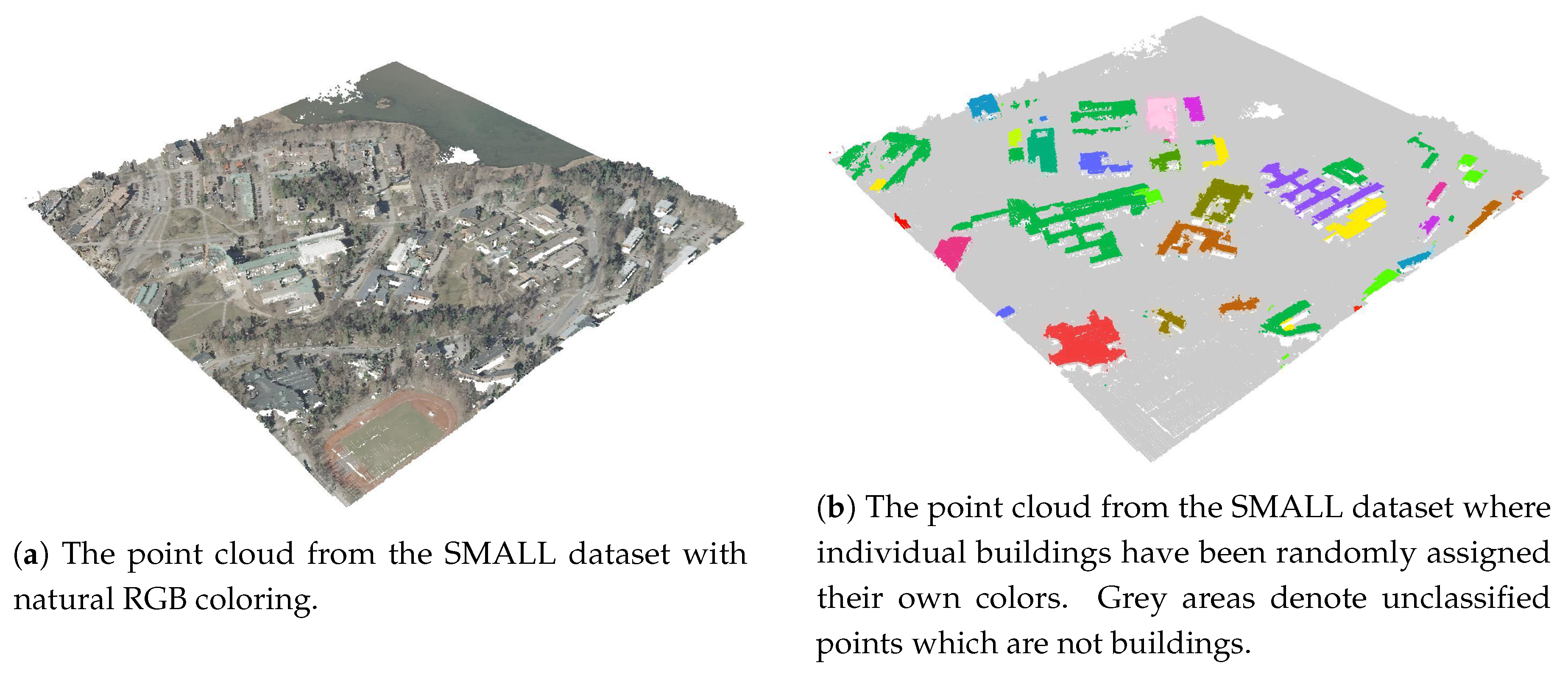
3.1. The Sample Point Clouds

We used three different point clouds of varying sizes, with the smallest dataset consisting of a few hundred thousand points and the largest containing nearly half a billion points. The datasets are referred to here as the (i) SMALL, (ii) MEDIUM and (iii) LARGE dataset and are briefly described in

Table 1. The three datasets that were used, of which the MEDIUM and LARGE are from Semantic3D.net [63].

SMALL Dataset	MEDIUM Dataset	LARGE Dataset
368,408 points representing the Otaniemi area in Espoo Finland. Source: National Land Survey of Finland, cropped sub-sample based on the ETR-TM35FIN coordinate system	29,697,591 points from Bildstein station, source: Semantic3D [63], file: bildstein_station1_xyz_intensity_rgb.7z.	496,702,861 points from a station, source: Semantic3D [63], file: sg27_station2_intensity_rgb.7z.

.

The SMALL dataset (Figure 1) differs slightly from the two other datasets with respect to the use of semantic $S_{ID}$. As its file is not obtained through Semantic3D [63], and  represents mostly buildings, $S_{ID}$ takes on here only two different values, namely 0 (no classification) or a large integer value that represents the building ID associated with each point. However, to be in line with the classification semantics of Semantic3D, we assume that each point in the SMALL dataset that is classified as a building is first associated with $S_{ID}=5$ and then also associated with a large integer value identifying a particular building. The SMALL dataset was downsampled so as to obtain a dataset that is clearly smaller than the MEDIUM dataset. In Section 4.1.1, we use the original, extended and non-downsampled SMALL dataset to test more complex queries. That dataset is used only in Section 4.1.1 and is referred to as the extended SMALL dataset. Therefore the term SMALL dataset, when used as such, is understood to refer to the downsampled SMALL dataset. The downsampled SMALL dataset contains a total of 84 buildings, each averaging roughly 500 points, with the rest of the points being unclassified. Other than this classification difference, the three datasets possess an identical file structure.

3.2. Using SDBL via Python

We assume that when querying point clouds, the user will be interested in objects belonging to a specific semantic class, such as finding certain buildings in a given location. (A list of potential semantic applications of points clouds is given in Reference [68]). In light of this, when SDBL is applied via Python, it basically means the data layout makes use of directories that reflect the various semantic classes while the queries are written in Python. More precisely, we first arrange the data according to the different semantic classes, so that for each distinct semantic label $S_{ID}$ 0 to 8, a separate directory named $ID\_S_{ID}$ is created, resulting in a total of nine separate directories.

For instance, the directory named ‘ID_0’ would include a file $Points$, which contains all the points whose semantic label $S_{ID}$ is equal to 0 (unclassified points), while in directory ‘ID_5’, the file $Points$ would contain only points whose semantic label $S_{ID}=5$ (i.e., buildings). It is worth noting that when using SDBL via Python and thus through directories, the semantic class $S_{ID}$ itself does not need to be stored in a file, since that information is already contained in the name of the directory ID_$S_{ID}$. To summarize, SDBL via Python is a layout where the previously mentioned file $Semantics$ has become unnecessary and the original $Points$ file that contained all the points in the dataset has now been decomposed into a new set of $Points$ files, with each $Points$ file residing in a sub-directory named ‘ID_$S_{ID}$’ so that all points in file $Points$ belong to the same semantic class $S_{ID}$. Finally, we note that to handle any particular query, the user is normally expected to supply at least the semantic class. However, it is possible to use this technique when the semantic ID or $S_{ID}$ is unknown as discussed in Section 4.3, although in such a case, the SDBL loses some of its inherent advantage that may lead to slower queries.

3.3. Using SDBL via PostgreSQL

To show that the basic idea in SDBL can also be used with a RDBMS, we implemented SDBL via PostgreSQL using the exact same three datasets. So as to use a data layout with tables that bears similarity to the basic idea behind SDBL, we use horizontal or row partitioning [69] to partition the data into a set of tables $T\_S_{ID}$ where $S_{ID}=0,1,2,\dots ,8$ so that each table $T\_S_{ID}$ stores points related to a single semantic class. Row partitioning, also known as horizontal fragmentation, is a technique that reduces the number of rows in a larger table by splitting the rows into a set of fragmented tables according to the common values of a partitioning attribute. In our case, the partitioning attribute is, of course, none other than the semantic ID attribute $S_{ID}$, meaning that the first fragmented table $T\_0$ will contain rows referring only to $S_{ID}=0$, the second fragmented table $T\_1$ will contain the rows referring only to $S_{ID}=1$, and so on. A partitioned or fragmented table $T_{S_{ID}}$ is thus made up of only rows that represent points that share a common semantic class $S_{ID}$. Once the dataset has been partitioned into a set of PostgreSQL tables, retrieving those points that are related to buildings ($S_{ID}=5$) in the MEDIUM dataset for instance amounts to running a simple SQL query such as SELECT * FROM T_MEDIUM_5, since all required points are now contained in the single fragmented table $T\_MEDIUM\_5$.

3.4. The Queries That Were Used

We ran five queries for the three different datasets, as depicted in

Table 2. The five different queries used for the SMALL dataset, which differ slightly from the ones used for the MEDIUM and LARGE datasets. Note that loading of points implies finding the correct set of points and loading them into memory.

Query ID	Description
Point Query $Q_1$	Load all points where $S_{ID}=5$ (buildings).
Point Query $Q_{1A}$	Load all points that refer to a particular building ID (ID = 416793804).
Point Query $Q_{1B}$	Load all points that refer to a particular building ID (ID = 41679427).
Rectangular Query $Q_3$	Load all points that refer to buildings and that are within a given rectangle.
Radial Query $Q_4$	Load all points that refer to buildings and that are within a given radius.

and 

Table 3. The five different queries used for the MEDIUM and LARGE datasets.

Query ID	Description
Point Query $Q_1$	Load all points where $S_{ID}=5$ (buildings).
Range $Q_{2A}$	Load all points that refer to buildings and where the x-coordinate $>20$
Point Query $Q_{2B}$	Load all points where $S_{ID}=2$ (natural terrain).
Rectangular Query $Q_3$	Load all points that refer to buildings and that are within a given rectangle.
Radial Query $Q_4$	Load all points that refer to buildings and that are within a given radius.

. For all three datasets, there was a basic (semantic) point query $Q_1$ that consisted of simply retrieving all the points associated with buildings. Since the SMALL dataset contained building IDs, two additional point queries ($Q_{1A}$ and $Q_{1B}$) that referred to two specific building IDs were used for this dataset, as shown in Table 2. We note in passing that while the authors in Reference [17] use the term point query to denote a query that retrieves a single point and its properties from the point cloud, we use it in the more broader spatial query sense to simply denote a query that requires an exact match (as opposed to a given range) for a certain attribute.

As for the MEDIUM (Figure 2) and LARGE (Figure 3) datasets, a range query $Q_{2A}$ was used to further restrict the results of point query $Q_1$ to find only those points whose X-coordinate was $>20$. As for point query $Q_{2B}$ (Table 3), it simply finds those points that are associated with $S_{ID}=2$ (natural terrain). For all three datasets, two range queries (illustrated in Figure 4) were tested, a rectangular query $Q_3$ and a radial query $Q_4$. Both of these queries use the result set from query $Q_1$, in other other words, they are applied to only those points that belong to buildings. The radial query $Q_4$ was so designed that for all three datasets, it would return a clearly smaller result set of points than query $Q_3$. Lastly, in order to get a feeling of how a point query that does not specify the semantic ID would fare, we ran an additional point query that retrieves a single point from the LARGE dataset as detailed in Section 4.3.

3.5. Querying the Data in SDBL Using Python

We assume that a data layout according to SDBL via Python has been created for a given dataset as outlined previously. Now when using SDBL via Python, querying all the points that are part of some building, that is, those with semantic class $S_{ID}=5$, amounts to simply reading the contents of a single file, namely the file $Points$ that is stored under the sub-directory named ‘ID_5’. A brief excerpt of the required Python code is shown in the Appendix A, Listing A1 where the function get_sem_xyz_points takes two parameters, cur_dir and semanticID, which refer to the data layout parent directory and to the semantic class respectively. Using the pandas [70] and feather packages [71], the function get_sem_xyz_points quickly reads (in line 5) a subset of the point cloud that is stored under the path supplied by the user in $cur\_dir$ and followed by sub-directory ‘ID_5’ (line 3) from a binary file (named ‘xyz.fff’ as shown in line 4). Thus, in order to obtain all the points that are related to buildings, one can simply issue the function call  get_sem_xyz_points (MyPath, ’5’) where MyPath refers to the directory containing the point cloud datasets. Applying a restriction and finding the set of desired points is accomplished via the pandas query function as shown in Listing A2.

We note that for the SMALL dataset, there would be additional sub-directories under the directory ‘ID_5’, with each sub-directory corresponding to a separate building ID as explained in Section 3.7. In order to test how the query times would be affected by increasing the number of sub-directories under the directory ‘ID_5’, we used the extended SMALL dataset. This test, along with the extended SMALL dataset, is described separately in Section 4.1.1.

3.6. Querying the Same SDBL Data in PostgreSQL

Querying using SDBL via PostgreSQL occurs through the fragmented tables as discussed previously in Section 3.3. While it is customary to retain the partitioning attribute in a fragmented table in case the tables need to be later rebuilt into the original unfragmented table, in our implementation we did not deem it necessary to include the column $S_{ID}$. The fragmented tables are thus each made up of four attributes, namely $(X,Y,Z,I)$. The SMALL dataset, as mentioned previously, is an exception in that all classified points refer to a specific building ID, so a semantic ID column does need to be included in table T_5 in order to hold the large integer values that identify a specific building. However, as the table for the SMALL dataset was rather small in size, a standard B-tree index on just the attributes $(X,Y,Z)$ was deemed enough, without resorting to the creation of a secondary index on $S_{ID}$.

It is worthwhile to note the difference between the just described horizontal partitioning and the patching (‘PC_PATCH’) [32] approach available in PostgreSQL (also found in Oracle as point cloud blocks). While patching reduces the index granularity by creating groups of co-located points, horizontal fragmentation reduces the number of rows in a given table without changing the index granularity. More importantly, fragmentation provides us with a mechanism of directly accessing semantic data since if all rows/points in a table share the same semantic ID, there is no longer the need to specify that attribute in a query.

Moreover, so as to get a better idea of the speed of the fragmented PostgreSQL table approach, we also used a PostGIS version of the fragmented approach in addition to the basic unfragmented approach, which acted as a benchmark for PostgreSQL queries. The unfragmented benchmark approach used a basic PostgreSQL table made up of five columns $(X,Y,Z,I,S)$ with a secondary index for column S, which refers to the semantic ID or $S_{ID}$.

Finally, for the SMALL dataset, we also tested a blocked Patch-table approach, which uses the PC_PATCH. In this approach, the building ID acts as a grouping attribute, so that each patch or block (there are 84 of them) is made up of points (an average of 500 points per patch) that belong to the same building ID. To make the Patch-table approach as fast as possible, we dropped the intensity column, so that the table effectively consisted of only four columns: the $(X,Y,Z)$ attributes and the semantic attribute $S_{ID}$.

In the following, we summarize the approaches that were used to test SDBL via PostgreSQL tables:

• Fragmented table: the dataset is fragmented into rows so that all points in a table belong to the same $S_{ID}$. The index is a basic B-tree composite $(X,Y,Z)$ non-clustered index. A total of nine fragmented tables are generated for the MEDIUM and the LARGE datasets, and only two fragmented tables ($S_{ID}=0$ and $S_{ID}=5$) for the SMALL dataset. The attributes in each fragment table are $(X,Y,Z,I)$.
• Fragmented PostGIS table (SMALL and MEDIUM datasets only): basically as above, but now the attributes are $(X,Y,Z)$ and S (for the SMALL dataset) and $(X,Y,Z)$ and I (for the MEDIUM dataset). These four attributes are incorporated into the PostGIS type ‘Point’. For the SMALL dataset, the index is made up of three separate functional indexes, which are for attributes X, Y and S (referring to $S_{ID}$). For the MEDIUM dataset, only two functional indexes are needed, for attributes X and Y. This PostGIS option is tested only for the SMALL and MEDIUM datasets, and only two fragmented tables (those that are actually queried) are generated for each dataset.
• Unfragmented benchmark table: the dataset, now comprised of attributes $(X,Y,Z,I,S)$ is contained in a single flat PostgreSQL table (without PostGIS) and without the use of fragmentation. This table acts as a benchmark for the other PostgreSQL tests and since it contains points from different semantic IDs, an additional B-tree index on attribute $S_{ID}$ was created in addition to the basic B-tree composite $(X,Y,Z)$ (non-clustered) index.
• Patch-table: this approach is only used with the SMALL dataset. The patches are created out of points that have the same building ID and the table is indexed via a GIST index on the PCPOINT type. The single patch-table contains the four attributes $(X,Y,Z,S)$.

3.7. Data Preparation for Using SDBL via Python

Before taking a look at the results in Section 4, we give some background on how the data was prepared to be used with SDBL. In order to prepare the point cloud datasets for use with SDBL via Python, we wrote a Python script (as specified in Section 3.9, we used Python version 3.7.1) that, for each of the datasets, partitions the data into directories according to the semantic class $S_{ID}$. For the MEDIUM and LARGE datasets, this means creating nine directories (one for each semantic class $S_{ID}$ in the range 0 to 8) and generating the file $Points(X,Y,Z,I)$ under each directory. For the SMALL dataset, this entails creating two main directories (one for semantic class $S_{ID}=0$ and for semantic class $S_{ID}=5$) and then creating under directory ‘ID_5’, a sub-directory ‘ID_BUILDING_ID’ for each separate BUILDING_ID (containing a separate $Points$ file for the building in question), resulting in a total of 84 sub-directories, the number of different buildings in the SMALL dataset.

For each dataset, the $Points$-files are stored separately on disk under the appropriate sub-directory using the fast binary feather format [71]. These files are then loaded into a pandas dataframe as needed for queries; the implicit index automatically created by pandas [70] was deemed sufficient and hence no explicit index was created.

Because in Section 4.3 we also tested queries that did not include the semantic class $S_{ID}$, we also store the minimum and maximum of X, Y and Z coordinates of each dataset in a separate file (a total of six values per each dataset). Having these six extreme values stored separately allows us not to have to load all nine $Points$-files when looking for a certain point $(X,Y,Z)$. In other words, should the point $(X,Y,Z)$ that is being queried not be contained within the stored minima and maxima, we can simply skip loading that particular $Points$-file.

3.8. Data Preparation for Using SDBL via PostgreSQL

As for preparing the data for PostgreSQL, we made use of the same Python script that was used to query SDBL via Python. Once a specific dataset had been prepared for Python use so that all nine $Points$ files had been written to their respective files using the feather package, the Python script was run and an option was chosen from the menu to convert the appropriate set of files into PostgreSQL tables. More precisely, the script used the SQLAlchemy [72] package to convert each $Points$ file into a corresponding fragmented PostgreSQL table. These tables were subsequently indexed via columns $(X,Y,Z)$.

Recall that the SMALL dataset is an exception in that the fragmented PostgreSQL table does contain a column S to hold the semantic ID ($S_{ID}$) which now refers to a building ID. Therefore, the preparation time for the SMALL dataset includes the time required to generate an additional B-tree index on attribute S using pgAdmin. For the MEDIUM and LARGE datasets however, all the data preparation for the fragmented PostgreSQL tables is done via the Python script.

As for the unfragmented PostgreSQL benchmark table, for each dataset, it was created using pgAdmin, indexed on $(X,Y,Z)$ and populated with data from the fragmented tables (using SQL). An additional index was then added on column S since an unfragmented table contains different semantic IDs.

We also tested PostGIS for the SMALL and MEDIUM datasets (without ‘PC_PATCH’). For the SMALL dataset, we created a PostGIS table with four attributes $(X,Y,Z,S)$ and populated it using the function PC_MAKEPOINT(1,ARRAY[X,Y,Z,S]) with data from a fragmented PostgreSQL table as shown in the Appendix A, in  Listing A5. Since S represents the building ID to which point $(X,Y,Z)$ belongs to, after  populating the SMALL dataset PostGIS table, a functional index was generated on three columns, namely X, Y and S.

As for using PostGIS with the MEDIUM dataset, two different PostGIS tables were generated, one fragmented with $S_{ID}=2$ and another fragmented with $S_{ID}=5$ (these two fragments were sufficient for the queries). These two tables contained the four attributes $(X,Y,Z,I)$ and were populated using the appropriate PostgreSQL fragmented table and the function PC_MAKEPOINT(1,ARRAY[X,Y,Z,I]). Once these two PostGIS tables were populated with their data, a functional index was generated for each table on just two columns, X and Y.

We note that the preparation times for SDBL via PostgreSQL using the fragmented tables approach as presented in Section 4 always include creating all possible table fragments. However, for the other PostGIS approaches, preparation times only include the time for creating the minimal fragments that are actually required for the queries.

Finally, ‘PC_PATCH’ was tested for the SMALL dataset only. This entailed creating patches according to the semantic ID value of those points where $S_{ID}=5$ using data from a PostGIS table fragment. The  table of patches was then indexed using a GIST index as shown in Listing A3.

3.9. The Software and Hardware That Was Used

A high performance Dell desktop (Precision 5820) with 64 GB RAM and a 3.6 GHz Xeon 6-core, running on a 64 bit Windows 10 and equipped with an internal 1 TB SSD for disk storage was used for all the tests. The software for the SDBL layout was written entirely in 64 bit Python (Python 3.7.1) using miniconda3 and making use of the pandas [70] and feather [71] packages.

As a RDBMS, we used PostgreSQL 10.8, together with pgAdmin (version 4.3) for running the queries. To evaluate the performance of a PostgreSQL query, the ‘Query Tool’ in pgAdmin was used to run each query. However, so as to obtain an accurate time, for each query we issued the command ‘EXPLAIN ANALYZE stmt’, where stmt is the query that was run. The query time is the sum obtained from the planning and execution times and it is these values which are reported in the result tables, that is,

Table 4. The data loading times along with the query times for five queries using the SMALL dataset. For the database implementation the query times for hot queries are shown in parenthesis. All times are in milliseconds.

Small Dataset (ms)	Preparation Time	Point Query ${\mathit{Q}}_1$	Point Query ${\mathit{Q}}_{2\mathit{A}}$	Point Query ${\mathit{Q}}_{2\mathit{B}}$	Rectangular Query ${\mathit{Q}}_3$	Radial Query ${\mathit{Q}}_4$
	Generate Semantic Files/Load Data	Points with Class ID = 5 (Buildings)	Points in Building with ID = 416793804	Points in Building with ID = 416794274	Points from Query ${\mathit{Q}}_{\mathbf{1}}$ within a Given Rectangle	Points from Query ${\mathit{Q}}_{\mathbf{1}}$ within a Given Radius
Python	3885	12.34	14.23	15.79	12.27	42.27
Fragmented table	4080	8.99 (3.46)	1.92 (0.32)	2.4 (0.42)	7.76 (5.35)	4.47 (1.99)
Fragmented PostGIS table	14,555	110.403 (107.952)	11.99 (4.17)	13.66 ( 5.66)	17.5 (16.03)	26.62 (16.81)
Unfragmented benchmark table (No PostGIS)	6919	53.88 (40.75)	1.77 (0.31)	2.16 (0.46)	205.14 (203.91)	52.94 (12.9)
Patch table	13,128	83.85 (79.00)	86.71 (81.47)	86.26 (72.24)	226.1 (207.81)	273.05 (177.93)
No of points returned	-	41,865	1386	1951	19,722	2556

(SMALL dataset),

Table 5. The preparation time along with the query times (in milliseconds) for five queries using the MEDIUM dataset. The fragmented table (without PostGIS) clearly provides for the fastest queries among the PostgreSQL approaches, even outperforming the Python approach for queries $Q_3$ and $Q_4$.

Medium Dataset (ms)	Preparation Time	Point Query ${\mathit{Q}}_1$	Range Query ${\mathit{Q}}_{2\mathit{A}}$	Point Query ${\mathit{Q}}_{2\mathit{B}}$	Rectangular Query ${\mathit{Q}}_3$	Radial Query ${\mathit{Q}}_4$
	Generate Semantic Files/Load Data	Points with Class ID = 5 (Buildings)	Points with Class ID = 5 and X > 20	Points with Class ID = 2 (Natural Terrain)	Points from Query ${\mathit{Q}}_{\mathbf{1}}$ within a Given Rectangle	Points from Query ${\mathit{Q}}_{\mathbf{1}}$ within a Given Radius
Python	43,806	46.53	62.48	93.39	109.344	108.67
Fragmented table	347,500	155.3 (153.61)	174.42 (154.93)	595.43 (444.49)	102.33 (59.60)	84.04 (42.77)
Fragmented PostGIS table	48,791	3311.96 (2330.27)	2123.12 (1999.72)	6307.97 (6106.05)	2758.13 (2618.52)	2207.35 (2123.22)
Unfragmented benchmark table (No PostGIS)	274,937	225.72 (154.99)	518.52 (188.78)	1009.53 (722.183)	327.3 (180.11)	381 (200.1)
No of points returned	-	1,242,205	385,664	3,508,530	261,911	68,160

(MEDIUM dataset),

Table 6. The preparation time along with the query times for five queries using the LARGE dataset. Quering using SDBL via Python is still the fastest approach for the simple queries $Q_1$, $Q_{2A}$ and $Q_{2B}$. All times are in seconds.

Large Dataset (s)	Preparation Time	Point Query ${\mathit{Q}}_1$	Range Query ${\mathit{Q}}_{2\mathit{A}}$	Point Query ${\mathit{Q}}_{2\mathit{B}}$	Rectangular Query ${\mathit{Q}}_3$	Radial Query ${\mathit{Q}}_4$
	Generate Semantic Files/Load Data	Points with Class ID = 5 (Buildings)	Points with Class ID = 5 and X > 20	Points with Class ID = 2 (Natural Terrain)	Points from Query ${\mathit{Q}}_{\mathbf{1}}$ within a Given Rectangle	Points from Query ${\mathit{Q}}_{\mathbf{1}}$ within a Given Radius
Python	426	1.37	3.44	3.06	3.64	5.65
Fragmented table	5882	27.87 (10.92)	10.56 (10.41)	61.43 (21.45)	1.83 (1.39)	1.15 (0.89)
Unfragmented benchmark table (No PostGIS)	9368	73.01 (22.49)	122.07 (22.5)	103.32 (72.18)	20.25 (2.43)	14.24 (1.23)
No of points returned	-	89,036,106	33,361,461	184,550,983	945,357	246,762

(LARGE dataset) and

Table 7. The time in milliseconds to locate a single point in the LARGE dataset. For the Python approach, the time in parentheses is the time needed to create an index after loading the file. For the two table approaches, the time in parentheses is the time for a hot query.

Point Query for Large Dataset (Returns a Single Point) (ms)	Python with Pandas (ms)	Fragmented Table (ms)	Unfragmented Table (ms)
Locating a specific point ($X=42.552,Y=94.641,Z=2.531$) that has $S_{ID}=6$ (hardscape).	7880 (47,710)	29.5 (1.5)	45.5 (0.22)

(special point-query without semantic ID). The hot queries for SDBL via PostgreSQL are shown in parentheses in these tables, the reported time for a hot query is the average of three runs for the query after the very first run, the so-called cold query.

4. Results

In the following sections, for each of the three datasets, we first present the results using SBDL via a Python approach followed by the results when using SBDL via fragmented tables PostgreSQL. The time required to prepare the dataset for Python is reported in the first column and first row of each of the results table (Table 4, Table 5 and Table 6).

4.1. The Results for the Small Dataset

The preparation time for the SMALL dataset when using SDBL via Python takes less than 4 s or 3885 ms as shown in Table 4 and is only very slightly faster than the preparation time for using the fragmented PostgreSQL table. The  preparation time for the latter, 4080 ms, is made up of the time to use the Python script to generate just two fragmented tables for $S_{ID}=0$ and $S_{ID}=5$ and index them on the attributes $(X,Y,Z)$ (requiring 3810 ms). Additionally, for the table fragment $S_{ID}=5$, we used pgAdmin to build a secondary index for attribute S in order to quickly retrieve the building IDs, an operation that required just 270 ms.

As for the data preparation time for the fragmented PostGIS tables (14,555 ms), it is made up of the time to create the two PostGIS table fragments $S_{ID}=0$ and $S_{ID}=5$ (605 ms), the time to populate them with corresponding data (2257 ms) from the PostgreSQL tables along with the time required to build three functional indexes on attributes X,Y and S (11,693 ms) for the table fragment $S_{ID}=5$ only.

The data preparation time for the unfragmented benchmark is nearly 7 s (6919 ms) and is made up of the time to create the table (177 ms), the time needed to add one semantic ID column and to index it (759 ms), along with the time to populate it with data (5983 ms) from the two fragmented PostgreSQL tables.

The query results for the SMALL dataset, also shown in Table 4, are unique in that for all queries, the fragmented table approach is faster than the Python approach. For instance, for the point query $Q_{2A}$, the Python approach requires 14.23 ms to retrieve into memory all the 1386 points that are contained in a single file (with building ID = 416793804). In contrast, the PostgreSQL query (Listing A4 in the Appendix A) is able to retrieve the same set of points from a fragmented table that contains all the points related to buildings in just 1.92 ms. We attribute this speed of PostgreSQL partly to the fact that the result set is in all queries relatively small, meaning a RDBMS can access the required data with a minimum of disk I/O operations. However, the Python query $Q_{2A}$ is also straightforward to execute, for it consists of mainly reading into memory a single binary file located under the sub-directory MyPath\ID_5\416793804\. In other words, there is no need to search for the correct $Points$ file, since its location is pre-determined from the building ID. Perhaps the Python approach is slightly slower than the fragmented PostgreSQL approach simply due to the additional overhead associated with the Python script, which comes into play when the query processing times are small.

The fragmented approach is for most queries clearly faster than the benchmark unfragmented approach, except for queries $Q_{2A}$ and $Q_{2B}$ which return a small result set and for which there is very little difference in the query times. For instance, for query $Q_{2A}$ the query times for the fragmented table and the benchmark table are respectively 1.92 ms and 1.77 ms.

Finally, we also tested the use of ‘PC_PATCH’ for point query $Q_1$ using the code in Listing A7. The results show that using patches or blocking does add to slowness, in fact the row marked ‘Patch table’ in Table 4 has the slowest query results throughout.

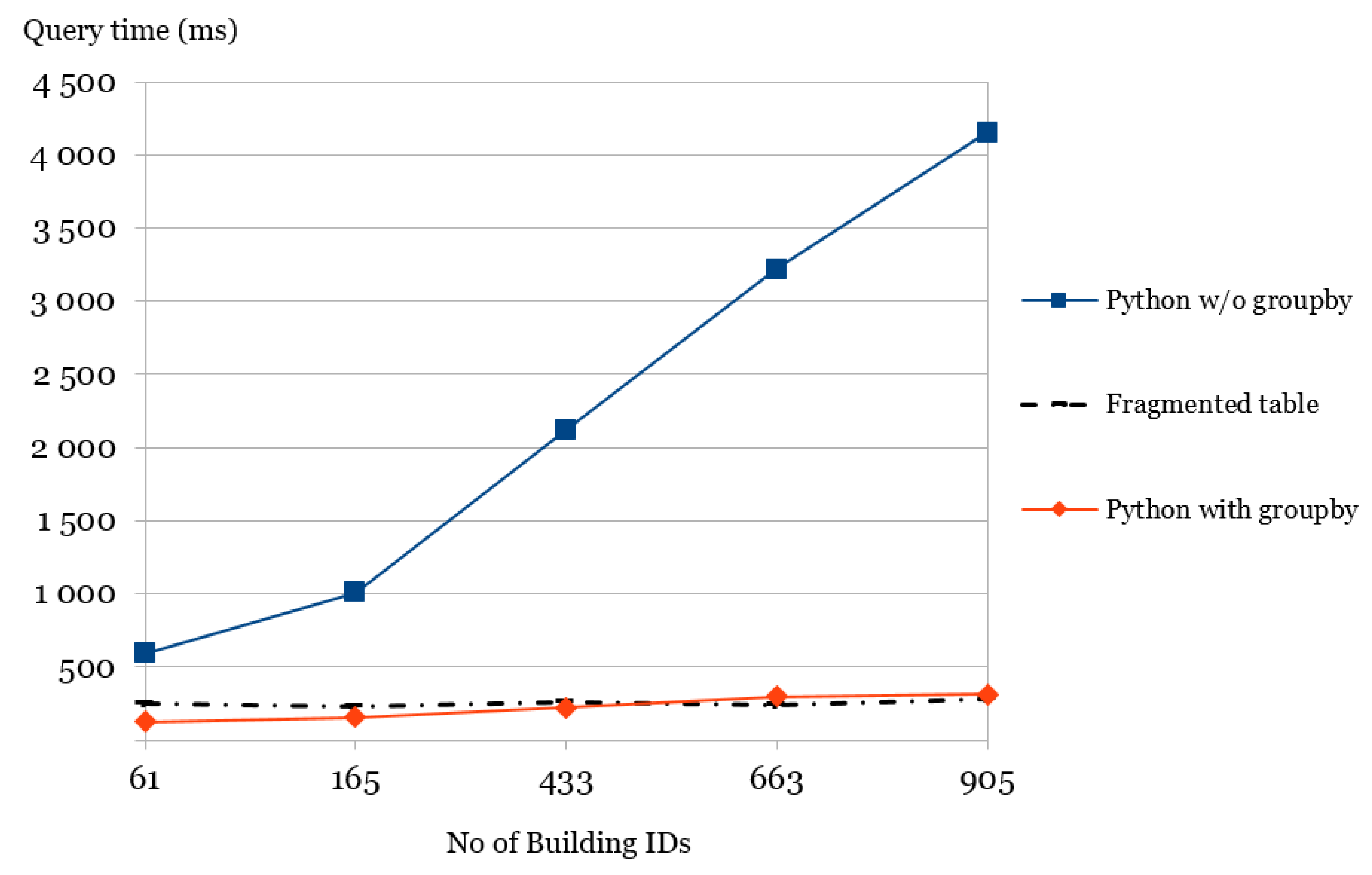
4.1.1. A More Complex Query Using the Extended Small Dataset

We recall that in the case of the SMALL dataset, SDBL via Python stores each $Points$ file for a given building ID under its own sub-folder (in addition to storing all the building IDs in a single larger $Points$ file under folder ‘ID_5’). Since it would be interesting to see the effect of a large number of sub-directories on a more complex query using the SDBL via Python, we resorted to using the extended version of the SMALL dataset. The extended version contains a larger geographic area with a higher point density, containing a total of 8,971,327 points representing 1940 different building IDs, which in turn, were comprised of a total of 906,926 points. We used a query that finds the maximum value for the Z-coordinate for each building ID in a basic $(X,Y$) range while excluding two particular building IDs. More precisely, we varied the range $X\ge X_{min}$ AND $Y\ge Y_{min}$ by using five different pairs of values for $X_{min}$ and $Y_{min}$ as shown in the ranges $R_1$–$R_5$ in

Table 8. The five more complex queries that access the extended small dataset and their completion times in milliseconds for three different implementations. The column ‘No of building IDs touched’ refers to the number of building IDs that contributed points towards the query. The hot query times for the fragmented table (fourth column) were almost identical to the cold query times and are therefore not shown.

Complex Queries (Five Different Ranges) Uses the Extended Small Dataset to locate the Max. Z-Coordinate in Each Building ID Other Than ID = ‘41679380’ and ID = ‘416794274’ in a Given $(\mathit{X},\mathit{Y})$ Region ${\mathit{R}}_{\mathit{x}}$, Defined Below.	No of Building IDs Touched	Python with Groupby (ms)	Fragmented Table (ms)	Python w/o Groupby (ms)
$R_1:X>=$ 379,020 and $Y>=$ 6,674,206	61	125	250	590
$R_2:X>=$ 379,520 and $Y>=$ 6,667,206	165	156	230	1010
$R_3:X>=$ 378,520 and $Y>=$ 6,667,206	433	219	260	2120
$R_4:X>=$ 378,200 and $Y>=$ 6,667,006	663	297	240	3220
$R_5:X>=$ 378,020 and $Y>=$ 6,664,206	905	310	280	4150

(while excluding building IDs ‘416793804’ and ‘416794274’). This effectively results in five queries.

Each of these five queries was run in three different implementations, with two Python variations, referred to as Python-with-groupby and Python-without-groupby and one fragmented PostgreSQL table implementation. The SQL query for the fragmented table case where $X_{min}=$ 378,020 and $Y_{min}=$ 6,664,206 is shown in Listing 2.

Although both Python implementations use SDBL via Python, they differ in how they access the data. The Python-with-groupby applies the pandas groupby function on a single dataframe that is obtained by reading a single larger $Points$ file under folder ‘ID_5’ (prior to applying the groupby function, the pandas query function was used to find the matching set of building IDs that fit the given $(X,Y)$ range and the two non-desired buiding IDs were excluded). The use of the pandas groupby is illustrated in Listing 1. The preparation time for both Python implementations was the same, 485 s, whereas the preparation time for the fragmented PostgreSQL table was obtained similarly as for the downsampled SMALL dataset and turned out to be 119 s.

Listing 1. Applying the pandas function groupby to the dataset Pts_BlockXY which contains the set of points in the desired range with the two unwanted buildings excluded as specified in the query of Section 4.1.1.

1 Pts_Block_grouped  =  Pts_BlockXY.loc[Pts_BlockXY.groupby(‘s’).z.idxmax()]
        

As for the Python-without-groupby approach, it processes each $Points$ file that meets the query criteria, albeit avoiding reading those $Points$ files whose extreme values for X and Y do not meet the given $(X,Y)$ range as described in Section 3.7. This effectively means that if one of the five queries over range $R_i$ returns $N_i$ building IDs, the Python-without-groupby will have read and processed $N_i$ $Points$ files. The three implementation approaches are briefly summarized below.

• Python-with-groupby: uses a single $Points$ file under folder ‘ID_5’ that is read into a dataframe. The dataframe is then pre-processed so that building IDs marked for exclusion in the query are dropped and only points within the given $(X,Y)$ range are included. Finally, the pandas groupby function is applied to the resulting dataframe to yield the final set of maximum Z-coordinate points (Pts_Block_grouped in Listing 1) for each building ID.
• Python-without-groupby: reads each $Points$ file from a separate sub-folder (under parent folder ‘ID_5’) that is within the given $(X,Y)$ range (and which does not belong to a building ID marked for exclusion) into a temporary dataframe df. From df, the maximum Z-coordinate is then computed and appended to a list to yield the final result.
• Fragmented table: uses a PostgreSQL table that contains all the points (rows) related to buildings, with a table structure that is identical to the one used for the downsampled SMALL dataset. The fragmented table contains 906,926 rows, the number of points related to buildings in the extended dataset.

The results are shown in Table 8 and in a graph format in Figure 5. From Table 8, it is seen that when the query touches (or refers to) a total of 61 buildings, all three queries complete well under 1 s, with Python-with-groupby and the fragmented table queries completing within 300 ms (125 ms and 250 ms respectively). The table also shows that when 905 building IDs are returned, the Python-with-groupby and fragmented table queries still complete in around 300 ms (310 ms and 280 ms respectively). However, the performance of the Python-without-groupby query has slowed down remarkably, taking over 3 s (3220 ms) to complete. This is attributed to the fact that the query actually needs to read and query 905 $Points$ files. As can be seen from the graph (Figure 5), the line-segment marked ‘Python without groupby’ sharply degrades in performance as the number of building IDs (and thus the number of $Points$ files) processed exceeds 165. This is in contrast with the Python-with-groupby approach which can always read all the building IDs from just a single $Points$ file.

Listing 2. The PostgreSQL complex query using the extended SMALL dataset for finding the highest Z-coordinate point among each building in a given (X,Y) region ($X\ge$ 378,020 and $X\ge$ 6,664,206), while excluding two building IDs (ID = ‘41679380’ and ID = ‘416794274’). Among the five range queries run, this query resulted in the largest number of building IDs, numbering 905.

1 EXPLAIN ANALYZE
2 SELECT MAX(Z) FROM P2xyz_s_5
3 WHERE X  > =  378020 AND  Y  > =  6664206
4 GROUP BY S HAVING S NOT IN (‘416793804’,‘416794274’)
        

4.2. The Results for the Medium Dataset

For the MEDIUM dataset, the results are shown in Table 5. The data is loaded into the fragmented PostgreSQL tables (time required is 43,806 ms) using a Python script similarly as with the SMALL dataset, except that the semantic ID is no longer stored in a table column since it now represents a semantic class (according to semantic3D [63]) and therefore all points/rows in a table share the same $S_{ID}$ value.

The preparation time for the fragmented PostGIS tables (48,791 ms) consisted of the time to create and populate the PostGIS fragments with attributes $(X,Y,Z,I)$ using data from the corresponding PostgreSQL fragments  (42,755 ms) and to create two functional indexes on X and Y for the fragment with $S_{ID}=5$ (requiring 6036 ms). The other fragments did not require functional indexes as no reference is made to their coordinates in the queries.

Regarding the preparation time for the unfragmented benchmark PostgreSQL table (274,937 ms), it consists of creating an empty table with columns $(X,Y,Z,I,S)$ (requiring 217 ms), populating the table with data from the nine fragmented tables (251,330 ms) and indexing it on the attribute $S_{ID}$ (23,390 ms).

Regarding the actual queries, the Python approach and the fragmented PostgreSQL approach clearly employ two entirely different different memory models: the former tries to keep the entire data in memory, while the latter fetches the required datapages from disk as needed. So it is interesting to note that with the MEDIUM dataset, although the Python approach is still relatively fast, for  the range queries $Q_3$ and $Q_4$, the fragmented PostgreSQL table approach is even slightly faster. For the point query $Q_{2B}$ that simply returns a large set of rows, the Python approach is clearly faster (93.39 vs. 595.43 ms). This is probably due to the fact that this particular query is processed through sequential reads which translate to about 40 disk page accesses (with a block size of 8 K) in order to read all the data for semantic class ID $S_{ID}=2$ (the table occupies 337 MB).

The fragmented PostGIS table approach is, as expected, clearly slower than the fragmented PostgreSQL approach, but also slower than the unfragmented benchmark PostgreSQL approach (which combines data from all the semantic IDs). This is at least partly due to the extra time required to convert the binary point representation into a more readable format with the help of the function PC_ASTEXT(pt) as shown in Listing A6.

4.3. The Results for the Large Dataset

We loaded the data into the fragmented PostgreSQL tables in the same way as was done with the MEDIUM dataset, and the large size of the dataset was clearly apparent in the required preparation time, which was now slightly over 1 $\mathrm{h}$  38 $\min$, or as shown in seconds in Table 6, 5882 s.

The preparation time for the unfragmented benchmark PostgreSQL table (9368 s), as with the MEDIUM dataset, consisted of creating an empty table with columns $(X,Y,Z,I,S)$ and populating it with data from the nine fragmented tables (requiring 8923 s) and indexing it on the attribute S (i.e., $S_{ID}$), requiring a further 445 s.

When examining the results of the LARGE dataset in Table 6, we recognize the same phenomenon that was visible with the previous MEDIUM dataset, whereby the fragmented table approach provides the fastest times for the range queries $Q_3$ and $Q_4$ but is markedly slower for other queries. What is noteworthy is that now the unfragmented table approach turns out to be markedly slower throughout than the fragmented tables. For instance, the times for the unfragmented and fragmented PostgreSQL query $Q_3$ are 20.25 s vs. 3.64 s and for query $Q_4$ 14.24 s vs. 5.65 s respectively.

As for using the SDBL via Python for point queries that return a single point without specifying $S_{ID}$ proved to be rather easy to achieve. We modified the Python script so that given a point $(X,Y,Z)$, it scans all nine semantic $Points$ files for the required point until it is found. And as mentioned in Section 3.7, we made use of the minima and maxima of $(X,Y,Z)$ for each semantic ID file so that a file was loaded into memory only if the point being queried was contained within the separarely stored minima and maxima.

Similarly, in order to use SDBL via PostgreSQL to query a single point without specifying $S_{ID}$, the fragmented table approach was simply extended through the use of the SQL union-operator in the query as shown in Listing 3. In such a case, the query assumes that the points to retrieve may be in any one (or several) table fragments, and therefore all nine ($S_{ID}$ 0 to 8) table fragments need to be queried. However, the results in Table 7 suggest that this is neither a complex nor slow query to process. For purposes of comparison, we also queried the unfragmented table (from the LARGE dataset) using the point query in Listing 4. The query for the fragmented table was slightly faster (29.5 ms) than the query for the unfragmented table (45.5 ms).

Listing 3. A PostgreSQL point query making use of the UNION-operator (range 0 to 8) for finding a given point without knowledge of its semantic ID.

1 EXPLAIN ANALYZE
2 SELECT * FROM P2xyz_L_0 WHERE X = 42.552 AND Y  =  94.641 AND Z  =  2.531
3 UNION
4 SELECT * FROM P2xyz_L_1 WHERE X = 42.552 AND Y  =  94.641 AND Z  =  2.531
5 ……
6 UNION
7 SELECT * FROM P2xyz_L_8 WHERE X = 42.552 AND Y  =  94.641 AND Z  =  2.531
        

Listing 4. A PostgreSQL point query that directly accesses a single point from a non-fragmented table that contains all points in the dataset.

1 EXPLAIN ANALYZE SELECT * FROM P2xyz_L WHERE X = 42.552
2 AND Y  =  94.641 AND Z  =  2.531
        

The results in Table 7 show that querying without a semantic ID certainly can be done rather easily. For the Python implementation, we also tried creating an explicit index on $(X,Y,Z)$, but the time required to create the index far outweighed any benefits as building the index and running the point query now took over 47 s  to complete (47,710 ms) as seen from Table 7. Running the same point query in Python using just the implicit index generated by pandas [70] proved to be satisfactory, and required 7780 ms.

5. Discussion and Conclusions

The SDBL approach was presented using two quite different formats, as it can be implemented via Python and pandas making use of directories or via the use of PostgreSQL as a RDBMS. The SDBL via Python approach can be characterized as a simple column-oriented store with the additional twist that semantic indexing is provided via the use of directories. The semantic3D data [63] with the semantic class stored for each point in a separate file (file $Semantics$) is helpful as the semantic information does not augment the size of the $Points$ file with the actual point cloud data. The SDBL via Python approach takes this semantic layout one step further by eliminating the need for the file $Semantics$ as the large $Points$ file gets decomposed into smaller $Points$ files that share the same semantic class and are stored in the same directory that carries the name of the semantic class.

On the other hand, the SDBL via PostgreSQL approach reduces the size of a relational table that holds point cloud data by fragmenting a larger table into smaller ones according to the semantic class: a particular table ends up containing rows or points that all belong to the same semantic ID. The two presented approaches, SDBL via Python and SDB via PostgreSQL also differ with respect to their memory model. When using SDBL via Python, the primary data working object is the pandas dataframe, which albeit its strong resemblance to a relational table in terms of its structure, is nevertheless non-persistent [73]. In other words, it is up to the programmer to choose a suitable data format (such as the feather package which we used) in order to save the dataframe onto disk for later use. The pandas package gets its speed from in-memory processing, that is, by attempting to keep all the required data in memory. This is in contrast with using SDBL via PostgreSQL, which gets its speed from the ability to quickly locate the correct data rows and then transfer the required disk blocks from disk into memory. We next briefly discuss the advantages and limitations of the two SDBL approaches.

5.1. Advantages of the Presented SDBL Approach

While breaking up large point clouds into smaller files—commonly known as tiling [23]—is useful as a means of archiving and distributing the point cloud data, it does impose an additional loading time which slows down queries considerably [74]. Moreover, tiling cannot guarantee that points belonging to the same semantic class will end up in the same tile file. In fact, different points of the same semantic object are bound to end up in separate tiles when the object’s edges cross the tile boundaries [75,76]. The SDBL via Python approach maintains semantic-based files and is therefore one way of overcoming this problem. Moreover, the SDBL via Python approach, though it is categorized as a column-oriented store, is easy to implement and maintain as it does not rely on any third-party big data tool (e.g., Hadoop). Compared to a file-based approach such as LAStools [77], SDBL via Python is likely to result in a much smaller set of files, even if there are hierarchies involved, for Reference [15] report that their test data set was comprised of over 60,000 files. Moreover, SDBL via Python is specifically designed for querying via semantic classes, and there is no need for an additional indexing mechanism since indexing is handled through the operating system: the different folders contain different semantic classes. These features give SDBL via Python an advantage over file-based solutions for queries where semantics play a fundamental role, such as in the fields of autonomous driving and industrial robotic applications [78] or when using indoor navigation or BIM (Building Information Modeling) [79].

As for using SDBL via PostgreSQL, Bayer, the father of the B-tree, has aptly pointed out [80] that the relational database model as such already incorporates multi-dimensionality. A record from a given table with n attributes can be seen as a point in space with n dimensions [80]. The challenge in using a RDBMS to store and effectively access point clouds therefore essentially rests on the index. More specifically, as we cannot assume that a large point cloud dataset will fit into memory, we would like that at least the index, or most of it, will be in memory so as to speed up queries. In fact, the authors of Reference [56] purposefully maintain the number of rows in a table below a few millions.

Reducing the total number of points/rows in a table through fragmentation is one way of achieving this. Moreover, fragmenting a table according to its semantic ID increases the likelihood that points that are co-located are stored contiguously on disk, thus eventually increasing the data retrieval speed. And as the results for the MEDIUM and LARGE datasets showed, the fragmented PostgreSQL approach is clearly faster than the unfragmented PostgreSQL approach for all queries. For the SMALL dataset, point queries $Q_{2A}$ and $Q_{2B}$ turn out to be slightly faster for the unfragmented PostgreSQL table than the fragmented tables PostgreSQL approach, but this small difference may be attributed to measurement inaccuracy as for the other queries in the SMALL dataset ($Q_1$, $Q_3$ and $Q_{2A}$) the fragmented tables approach is clearly faster than the unfragmented table approach.

If there is no compelling need to use a RDBMS for storing a point cloud, then using SDBL programmatically with Python (along with the pandas and feather packages) and directories should provide satisfactory results. The use of directories and their naming according to $S_{ID}$ provides for a quick way of locating data based on semantic classes. The benefits is that indexing is now effectively taken care of by the underlying operating system, which is responsible for file and directory management. The idea of using directories as the indexing-mechanism is taken from our previous work  [81].

5.2. Limitations of the Presented SDBL Approach

Though we did not use the color attributes $(R,G,B)$, the presented approach does not actually limit their use. Including the color attributes will, of course, result in slightly larger files/tables and hence it is likely that there will be a noticeable reduction in the speed of the queries related to large datasets. In fact, the current implementation for the MEDIUM dataset (that did not use colors) was successfully run in a configuration with only 8GB of RAM, albeit with much slower query times.

While the presented approach is built on the premise that each query includes the semantic ID, it is possible to apply it to point queries that do not specify the $S_{ID}$, as was shown in Section 4.3. In this respect, we do not foresee any major obstacle in using SDBL in various applications. However, if SDBL via Python is used with a set of several queries where each query refers to a different semantic ID, this will imply that for each query, the data will need to be loaded from a file into a pandas dataframe (in memory) for the purpose of a single query. Though SDBL should be of benefit here in that it reduces the size of the files, the Python script will nevertheless need to load each $Points$ file from disk for the purpose of running a single query. As the Semantic3D format uses a total of nine semantic classes, without  sub-hierarchies, the maximum number of $Points$ files will not therefore exceed nine.

The results for the more complex query type using the extended SMALL dataset in Section 4.1.1 show that if a relatively large number (say well over 100) of $Points$ files are read, the performance of Python via SDBL quickly degenerates into a file-based approach, meaning that the advantages gained by the memory-based pandas dataset approach are lost. However, in the case of sub-hierarchies and a query that accesses a large number of semantic sub-classes (i.e., building IDs), this situation can easily be remedied by using a single larger $Points$ file that resides in the parent folder and contains all points in the sub-folders. This approach is effectively the one used for the Python-with-groupby query (Section 4.1.1); it should also prove useful when using queries that involve points in boundary semantic classes (such as a building and the ground underneath it).

Should such $Points$ files become very large (say well over 200 million rows), the query times could be made faster by breaking up the semantic ID classes in question into a sub-hierarchy, which in turn could be stored in corresponding sub-directories. So for instance, the semantic class for buildings could be further classified into a sub-hierarchy of roofs and façades as was done in Reference [82]. This arrangement should prove useful provided the query needs to access specific semantic objects and care is taken to avoid the problem of accessing too many $Points$ files in a query as previously discussed. The use of a sub-hierarchy can also be used to counteract the fact that the distribution of the semantic IDs is likely to be uneven for the different semantic classes [78].

Finally, as this study was limited to using easily deployable, one node solutions, we did not test how SBDL would benefit from parallel processing.

5.3. How the Presented SDBL Approach Relates to Previous Work

In their articles [56,83] on creating a point cloud server, Cura et al. envisage grouping point clouds according to various properties, including semantic data. The authors note that if for instance building data is grouped together, care must be taken not to have too large a group since finding a particular point would then entail reading the whole group [56]. The benefit in using SDBL via Python is that the data related to the active $S_{ID}$ is likely to be in memory. As an example, if the user issues a query related to buildings, the building dataset remains in memory (as a pandas dataframe) until the user switches the semantic ID to some other target such as high vegetation $(S_{ID}=3)$.

Cura et al. [56] use a RDBMS (PostgreSQL and PostGIS) where the number of points is reduced through patching and refer to their interesting design as PCS, short for Point Cloud Server. However, unlike with our SDBL via PostgreSQL, using PCS does not require that all points in a patch belong to the same semantic class. Moreover, SDBL via PostgreSQL does not use patches or compress the points. Interestingly, PCS makes use of functional indexes to allow querying patches of points without exploding them. Whenever a new patch is generated, several functional indexes on different properties are computed and stored in a ‘simplified format’ (with less accuracy and hence less space) in the database. It then becomes possible to disregard whole patches of points (e.g., those that are not buildings) without exploding them [56]. When a suitable patch is found however, its points do of course need to be exploded in order to be retrieved. The query times reported for the PCS approach separate the process of finding a patch from actually retrieving and unpacking it [56] and therefore the times provided are not directly comparable with our approach.

Van Oosterom et al. [15] conducted a large and detailed benchmark on querying very large point clouds that includes using PostgreSQL (without patches) and PostGIS with patches. In one of their rectangular queries (query no 2) on dataset ‘210M’, (210,631,597 points) using PostgreSQL with patches and with no additional attributes besides $(X,Y,Z)$, the authors reported a hot query time of 2.15 s (the authors used a powerful server with 128 GB RAM and 2 × 8-core Intel Xeon processors) for a query that returned 563,108 points. In contrast, our SDBL via PostgreSQL fragmented rectangular query that returned 945,357 points completed in 1.39 s for the LARGE dataset (total of nearly half a billion points). It should come as no suprise that the query times we found for the fragmented PostgreSQL approach are competitive with query times for a similar query using PostGIS with patches that was run in a more powerful hardware platform. After all, since the SBDL via PostgreSQL query assumes that all points in the rectangular area belong to the same semantic class, it can therefore make use of a fragmented table that is much smaller row-wise (only 8,903,610 rows) than the total number of points in the dataset.

In Reference [25], Poux et al. define a framework for a Smart Point Cloud or SPC which separates the semantics from the geographical within a framework of three classes. SPC uses an interesting semantic classification scheme where each point is classified at level 0 if it relates to the ground or other boundaries such as walls and ceilings. When the point is part of an object $O_1$ that rests on the ground (such as a table), it is classified at level 1 and, if the object $O_1$ acts as a host to another object $O_2$, then that object $O_2$ is known as the first guest and is classified at a level immediately above, that is, level 2 in this case [25]. Such a scheme should prove very useful for indoor point cloud segmentation [79] and could be implemented using SDBL via Python for instance.

In Reference [84], Poux details how a point cloud can be processed so as to extract the semantic data and store it into a point cloud database (PostgreSQL V.9.6) for semantic queries. The author shows how an SQL point query would return the name of the object that hosts the given point. However, the emphasis of the work is on classifying the semantics of a point cloud efficiently (an area of 68 rooms is analyzed and classified in just 59 min) rather than querying.

5.4. Future Directions

It would be interesting to test the presented SDBL via a Python and via a PostgreSQL approach with a large, real world point cloud dataset that would incorporate semantic ID hierarchies. For instance, if  buildings are further classified into roof and façades, this would simply require the use of two additional sub-directories for the SBDL via Python approach and the use of two additional fragmented tables for the SBDL via PostgreSQL approach. One would expect that the query times would not become significantly slower, and  testing this premise should make for a promising future research project.

References

1. Vo, A.V.; Laefer, D.F.; Bertolotto, M. Airborne laser scanning data storage and indexing: State-of-the-art review. Int. J. Remote Sens. 2016, 37, 6187–6204. [Google Scholar] [CrossRef] [Green Version]
2. Haala, N.; Petera, M.; Jens Kremerb, G.H. Mobile LiDAR mapping for 3D point cloud collection in urban: A performance test. Int. Arch. Photogramm. Remote Sens. Spat. Inf. Sci. 2008, 37, 1119–1124. [Google Scholar] [CrossRef] [Green Version]
3. Kukko, A.; Kaartinen, H.; Hyyppä, J.; Chen, Y. Multiplatform Mobile Laser Scanning: Usability and Performance. Sensors 2012, 12, 11712–11733. [Google Scholar] [CrossRef] [Green Version]
4. Remondino, F.; Spera, M.G.; Nocerino, E.; Menna, F.; Nex, F. State of the art in high density image matching. Photogramm. Rec. 2014, 29, 144–166. [Google Scholar] [CrossRef] [Green Version]
5. Khoshelhamand, K.; Elberink, S.O. Accuracy and Resolution of Kinect Depth Data for Indoor Mapping Applications. Sensors 2012, 12, 1437–1454. [Google Scholar] [CrossRef] [PubMed] [Green Version]
6. Weinmann, M.; Schmidt, A.; Mallet, C.; Hinz, S.; Rottensteiner, F.; Jutzi, B. Contextual Classification of Point Cloud Data by Exploiting Individual 3D Neighborhoods. ISPRS Ann. Photogramm. Remote Sens. Spat. Inf. Sci. 2015, 271–278. [Google Scholar] [CrossRef] [Green Version]
7. Koppula, H.S.; Anand, A.; Joachims, T.; Saxena, A. Semantic Labeling of 3D Point Clouds for Indoor Scenes. In Advances in Neural Information Processing Systems, Proceedings of the 25th Annual Conference on Neural Information Processing Systems (NIPS 2011), Granada, Spain, 12–14 December 2011; Shawe-Taylor, J., Zemel, R.S., Bartlett, P.L., Pereira, F.C.N., Weinberger, K.Q., Eds.; Curran Associates: Red Hook, NY, USA, 2011; pp. 244–252. [Google Scholar]
8. Virtanen, J.P.; Kukko, A.; Kaartinen, H.; Jaakkola, A.; Turppa, T.; Hyyppä, H.; Hyyppä, J. Nationwide Point Cloud—The Future Topographic Core Data. ISPRS Int. J. Geo-Inf. 2017, 6, 243. [Google Scholar] [CrossRef]
9. Ekman, P. Scene Reconstruction from 3D Point Clouds. Master’s Thesis, Aalto University School of Science, Espoo, Finland, 2017. [Google Scholar]
10. Chu, E.; Beckmann, J.; Naughton, J. The Case for a Wide-table Approach to Manage Sparse Relational Data Sets. In Proceedings of the 2007 ACM SIGMOD International Conference on Management of Data (SIGMOD ’07), Beijing, China, 12–14 June 2007; ACM: New York, NY, USA, 2007; pp. 821–832. [Google Scholar] [CrossRef]
11. Alvanaki, F.; Goncalves, R.; Ivanova, M.; Kersten, M.; Kyzirakos, K. GIS Navigation Boosted by Column Stores. Proc. VLDB Endow. 2015, 8, 1956–1959. [Google Scholar] [CrossRef]
12. Ramamurthy, R.; DeWitt, D.J.; Su, Q. A Case for Fractured Mirrors. VLDB J. 2003, 12, 89–101. [Google Scholar] [CrossRef]
13. Asano, T.; Ranjan, D.; Roos, T.; Welzl, E.; Widmayer, P. Space-filling Curves and Their Use in the Design of Geometric Data Structures. Theor. Comput. Sci. 1997, 181, 3–15. [Google Scholar] [CrossRef] [Green Version]
14. Kim, J.; Seo, S.; Jung, D.; Kim, J.S.; Huh, J. Parameter-Aware I/O Management for Solid State Disks (SSDs). IEEE Trans. Comput. 2012, 61, 636–649. [Google Scholar] [CrossRef]
15. van Oosterom, P.; Martinez-Rubi, O.; Ivanova, M.; Horhammer, M.; Geringer, D.; Ravada, S.; Tijssen, T.; Kodde, M.; Gonçalves, R. Massive Point Cloud Data Management. Comput. Graph. 2015, 49, 92–125. [Google Scholar] [CrossRef]
16. Psomadaki, S. Using a Space Filling Curve for the Management of Dynamic Point Cloud Data in a Relational DBMS. Master’s Thesis, Delft University of Technology, Delft, The Netherlands, 2016. [Google Scholar]
17. Vo, A.V.; Konda, N.; Chauhan, N.; Aljumaily, H.; Laefer, D.F. Lessons learned with laser scanning point cloud management in Hadoop HBase. In Advanced Computing Strategies for Engineering, Proceedings of the 25th EG-ICE International Workshop 2018, Lausanne, Switzerland, 10–13 June 2018; Smith, I.F.C., Domer, B., Eds.; Springer: Berlin/Heidelberg, Germany, 2018; Part II; pp. 1–16. [Google Scholar]
18. Sippu, S.; Soisalon-Soininen, E. Transaction Processing: Management of the Logical Database and Its Underlying Physical Structure; Springer: Berlin, Germany, 2015. [Google Scholar]
19. Richter, R.; Döllner, J. Concepts and techniques for integration, analysis and visualization of massive 3D point clouds. Comput. Environ. Urban Syst. 2014, 45, 114–124. [Google Scholar] [CrossRef]
20. Isenburg, M. LASzip: Lossless Compression of Lidar Data. Photogramm. Eng. Remote Sens. 2013, 79, 209–217. [Google Scholar] [CrossRef]
21. van Oosterom, P.; Martinez-Rubi, O.; Tijssen, T.; Gonçalves, R. Realistic Benchmarks for Point Cloud Data Management Systems. In Advances in 3D Geoinformation. Lecture Notes in Geoinformation and Cartography; Abdul-Rahman, A., Ed.; Springer: Cham, Swizerland, 2017; pp. 1–30. [Google Scholar] [CrossRef]
22. Martinez-Rubi, O.; van Oosterom, P.; Gonçalves, R.; Tijssen, T.; Ivanova, M.; Kersten, M.L.; Alvanaki, F. Benchmarking and Improving Point Cloud Data Management in MonetDB. SIGSPATIAL Spec. 2014, 6, 11–18. [Google Scholar] [CrossRef] [Green Version]
23. Boehm, J. File-centric Organization of large LiDAR Point Clouds in a Big Data context. In Proceedings of the IQmulus 1st Workshop on Processing Large Geospatial Data, Cardiff, UK, 8 July 2014; pp. 69–76. [Google Scholar]
24. Guan, X.; Van Oosterom, P.; Cheng, B. A Parallel N-Dimensional Space-Filling Curve Library and Its Application in Massive Point Cloud Management. ISPRS Int. J. Geo-Inf. 2018, 7, 327. [Google Scholar] [CrossRef] [Green Version]
25. Poux, F.; Hallot, P.; Neuville, R.; Billen, R. Smart point cloud: Definition and remaining challenges. ISPRS Ann. Photogramm. Remote Sens. Spat. Inf. Sci. 2016, IV-2/W1, 119–127. [Google Scholar] [CrossRef] [Green Version]
26. Chamberlin, D.D.; Boyce, R.F. SEQUEL: A Structured English Query Language. In Proceedings of the 1974 ACM SIGFIDET (Now SIGMOD) Workshop on Data Description, Access and Control (SIGFIDET ’74), Ann Arbor, MI, USA, May 1974; ACM: New York, NY, USA, 1974; pp. 249–264. [Google Scholar] [CrossRef]
27. Codd, E.F. A Relational Model of Data for Large Shared Data Banks. Commun. ACM 1970, 13, 377–387. [Google Scholar] [CrossRef]
28. Bayer, R.; McCreight, E. Organization and Maintenance of Large Ordered Indices. In Proceedings of the 1970 ACM SIGFIDET (Now SIGMOD) Workshop on Data Description, Access and Control, SIGFIDET ’70, Rice University, Houston, TX, USA, July 1970; ACM: New York, NY, USA, 1970; pp. 107–141. [Google Scholar] [CrossRef]
29. Schön, B.; Bertolotto, M.; Laefer, D.F.; Morrish, S. Storage, manipulation, and visualization of LiDAR data. In Proceedings of the 3rd ISPRS International Workshop 3D-ARCH 2009, Trento, Italy, 25–28 February 2009. [Google Scholar]
30. PostgreSQL 11.2 Documentation. Documentation, The PostgreSQL Global Development Group, USA. 2019. Available online: https://www.postgresql.org/files/documentation/pdf/11/postgresql-11-A4.pdf (accessed on 15 October 2019).
31. Blasby, D. Building a Spatial Database in PostgreSQL. Report, Refractions Research. 2001. Available online: http://postgis.refractions.net/ (accessed on 15 October 2019).
32. Ramsey, P. LIDAR in PostgreSQL with PointCloud. Available online: http://s3.cleverelephant.ca/foss4gna2013-pointcloud.pdf (accessed on 15 October 2019).
33. Zicari, R.V. Big Data: Challenges and Opportunities. In Big Data Computing; Akerkar, R., Ed.; CRC Press, Taylor & Francis Group: Boca Raton, FL, USA, 2014; pp. 103–128. [Google Scholar]
34. Sicular, S. Gartner’s Big Data Definition Consists of Three Parts, Not to Be Confused with Three ’V’s. Available online: http://businessintelligence.com/bi-insights/gartners-big-data-definition-consists-of-three-parts-not-to-be-confused-with-three-vs/ (accessed on 3 September 2019).
35. Zicari, R.V.; Rosselli, M.; Ivanov, T.; Korfiatis, N.; Tolle, K.; Niemann, R.; Reichenbach, C. Setting Up a Big Data Project: Challenges, Opportunities, Technologies and Optimization. In Big Data Optimization: Recent Developments and Challenges, Studies in Big Data 18; Emrouznejad, A., Ed.; Springer: Cham, Switzerland, 2016; pp. 17–45. [Google Scholar] [CrossRef]
36. Evans, M.R.; Oliver, D.; Zhou, X.; Shekhar, S. Spatial Big Data: Case Studies on Volume, Velocity and Variety. In Big Data: Techniques and Technologies in GeoInformatics; Karimi, H.A., Ed.; Taylor and Francis: Boca Raton, FL, USA, 2010; pp. 149–173. [Google Scholar]
37. Wadkar, S.; Siddalingaiah, M. Pro Apache Hadoop; Apress: New York, NY, USA, 2014. [Google Scholar]
38. Cattell, R. Scalable SQL and NoSQL Data Stores. SIGMOD Rec. 2011, 39, 12–27. [Google Scholar] [CrossRef] [Green Version]
39. Gessert, F.; Wingerath, W.; Friedrich, S.; Ritter, N. NoSQL Database Systems: A Survey and Decision Guidance. Comput. Sci. 2017, 32, 353–365. [Google Scholar] [CrossRef]
40. Hecht, R.; Jablonski, S. NoSQL Evaluation: A Use Case Oriented Survey. In Proceedings of the 2011 International Conference on Cloud and Service Computing (CSC ’11), Hong Kong, China, 12–14 December 2011; IEEE Computer Society: Washington, DC, USA, 2011; pp. 336–341. [Google Scholar] [CrossRef]
41. Davoudian, A.; Chen, L.; Liu, M. A Survey on NoSQL Stores. ACM Comput. Surv. 2018, 51, 40:1–40:43. [Google Scholar] [CrossRef]
42. Héman, S. Updating Compressed Column-Stores. Ph.D. Thesis, Vrije Universiteit Amsterdam, Amsterdam, The Netherlands, 2015. [Google Scholar]
43. Wang, Y.; Sun, Y.; Liu, Z.; Sarma, S.E.; Bronstein, M.M.; Solomon, J.M. Dynamic Graph CNN for Learning on Point Clouds. ACM Trans. Graph. 2019, 38, 146:1–146:12. [Google Scholar] [CrossRef] [Green Version]
44. Xiang, L.; Shao, X.; Wang, D. Providing R-Tree Support for MongoDB. Int. Arch. Photogramm. Remote Sens. Spatial Inf. Sci. 2016, XLI-B4, 545–549. [Google Scholar] [CrossRef]
45. Dean, J.; Ghemawat, S. MapReduce: Simplified Data Processing on Large Clusters. Commun. ACM 2008, 51, 107–113. [Google Scholar] [CrossRef]
46. Dean, J.; Ghemawat, S. MapReduce: A Flexible Data Processing Tool. Commun. ACM 2010, 53, 72–77. [Google Scholar] [CrossRef]
47. Santos, M.Y.; Costa, C.; Galvão, J.A.; Andrade, C.; Martinho, B.A.; Lima, F.V.; Costa, E. Evaluating SQL-on-Hadoop for Big Data Warehousing on Not-So-Good Hardware. In Proceedings of the 21st International Database Engineering & Applications Symposium, IDEAS 2017, Bristol, UK, 12–14 July 2017; ACM: New York, NY, USA, 2017; pp. 242–252. [Google Scholar] [CrossRef]
48. Floratou, A.; Minhas, U.F.; Özcan, F. SQL-on-Hadoop: Full Circle Back to Shared-nothing Database Architectures. Proc. VLDB Endow. 2014, 7, 1295–1306. [Google Scholar] [CrossRef] [Green Version]
49. Armbrust, M.; Xin, R.S.; Lian, C.; Huai, Y.; Liu, D.; Bradley, J.K.; Meng, X.; Kaftan, T.; Franklin, M.J.; Ghodsi, A.; et al. Spark SQL: Relational Data Processing in Spark. In Proceedings of the 2015 ACM SIGMOD International Conference on Management of Data, SIGMOD ’15, Melbourne, VIC, Australia, 31 May–4 June 2015; ACM: New York, NY, USA, 2015; pp. 1383–1394. [Google Scholar] [CrossRef]
50. Pajic, V.; Govedarica, M.; Amovic, M. Model of Point Cloud Data Management System in Big Data Paradigm. ISPRS Int. J. Geo-Inf. 2018, 7, 265. [Google Scholar] [CrossRef] [Green Version]
51. Comer, D. The Ubiquitous B-Tree. ACM Comput. Surv. 1979, 11, 121–137. [Google Scholar] [CrossRef]
52. Wedekind, H. On the selection of access paths in a data base system. In Proceedings of the IFIP Working Conference Data Base Management, Cargese, Corsica, France, 1–5 April 1974; Klimbie, J., Koffeman, K., Eds.; North-Holland: Amsterdam, The Netherlands, 1974; pp. 385–397. [Google Scholar]
53. Johnson, T.; Shasha, D. B-trees with Inserts and Deletes: Why Free-at-empty is Better Than Merge-at-half. J. Comput. Syst. Sci. 1993, 47, 45–76. [Google Scholar] [CrossRef] [Green Version]
54. Garcia-Molina, H.; Ullman, J.D.; Widom, J. Database System Implementation; Prentice-Hall: Upper Saddle River, NJ, USA, 2000. [Google Scholar]
55. Ooi, B.C.; Tan, K.L.; Tan, K.L. B-trees: Bearing Fruits of All Kinds. Aust. Comput. Sci. Commun. 2002, 24, 13–20. [Google Scholar]
56. Cura, R.; Perret, J.; Paparoditis, N. A scalable and multi-purpose point cloud server (PCS) for easier and faster point cloud data management and processing. ISPRS J. Photogramm. Remote Sens. 2017, 127, 39–56. [Google Scholar] [CrossRef]
57. Terry, J. Indexing Multidimensional Point Data. Ph.D. Thesis, Institute for Integrated and Intelligent Systems, Griffith University, South Brisbane, Australia, 2008. [Google Scholar]
58. Bayer, R.; Markl, V. The UB-Tree: Performance of Multidimensional Range Queries; Technical Report, Institut für Informatik; TU München: Munich, Germany, 1999. [Google Scholar]
59. Lawder, J. The Application of Space-filling Curves to the Storage and Retrieval of Multi-Dimensional Data. Ph.D. Thesis, University of London (Birkbeck College), London, UK, 2000. [Google Scholar]
60. Mokbel, M.F.; Aref, W.G. Irregularity in Multi-dimensional Space-filling Curves with Applications in Multimedia Databases. In Proceedings of the Tenth International Conference on Information and Knowledge Management (CIKM ’01), Atlanta GA, USA, 5–10 October 2001; ACM: New York, NY, USA, 2001; pp. 512–519. [Google Scholar] [CrossRef] [Green Version]
61. Ghane, A. The Effect of Reordering Multi-Dimensional Array Data on CPU Cache Utilization. Master’s Thesis, Simon Fraser University, Burnaby, BC, Canada, 2013. [Google Scholar]
62. Dandois, J.P.; Baker, M.; Olano, M.; Parker, G.G.; Ellis, E.C. What is the Point? Evaluating the Structure, Color, and Semantic Traits of Computer Vision Point Clouds of Vegetation. Remote Sens. 2017, 9, 355. [Google Scholar] [CrossRef] [Green Version]
63. Hackel, T.; Savinov, N.; Ladicky, L.; Wegner, J.D.; Pollefeys, K.S.M. Semantic3D.net: A new Large-scale Point Cloud Classification Benchmark. ISPRS Ann. Photogramm. Remote Sens. Spat. Inf. Sci. 2017, II-3/W4, 91–98. [Google Scholar] [CrossRef] [Green Version]
64. Weinmann, M.; Weinmann, M.; Schmidt, A.; Mallet, C.; Bredif, M. A Classification-Segmentation Framework for the Detection of Individual Trees in Dense MMS Point Cloud Data Acquired in Urban Areas. Remote Sens. 2017, 9, 277. [Google Scholar] [CrossRef] [Green Version]
65. Pusala, M.K.; Salehi, M.A.; Katukuri, J.R.; Xie, Y.; Raghavan, V. Massive Data Analysis: Tasks, Tools, Applications, and Challenges. In Advances in 3D Geoinformation. Lecture Notes in Geoinformation and Cartography; Springer: New Delhi, India, 2016; pp. 11–40. [Google Scholar]
66. National Land Survey of Finland. Maps and Spatial Data. Available online: https://www.maanmittauslaitos.fi/en/maps-and-spatial-data/expert-users/product-descriptions/laser-scanning-data (accessed on 3 December 2019).
67. National Land Survey of Finland. Topographic Database. Available online: https://www.maanmittauslaitos.fi/en/maps-and-spatial-data/expert-users/product-descriptions/topographic-database (accessed on 3 December 2019).
68. Poux, F.; Neuville, R.; Nys, G.A.; Billen, R. 3D Point Cloud Semantic Modelling: Integrated Framework for Indoor Spaces and Furniture. Remote Sens. 2018, 10, 1412. [Google Scholar] [CrossRef] [Green Version]
69. Al-Kateb, M.; Sinclair, P.; Au, G.; Ballinger, C. Hybrid Row-column Partitioning in Teradata. Proc. VLDB Endow. 2016, 9, 1353–1364. [Google Scholar] [CrossRef] [Green Version]
70. McKinney, W. Pandas: Powerful Python Data Analysis Toolkit. Available online: https://pandas.pydata.org/pandas-docs/stable/pandas.pdf (accessed on 12 December 2019).
71. Ramm, J. feather Documentation Release 0.1.0. Available online: https://buildmedia.readthedocs.org/media/pdf/plume/stable/plume.pdf (accessed on 12 December 2019).
72. Bayer, M. SQLAlchemy Documentation: Release 1.0.12. Available online: https://buildmedia.readthedocs.org/media/pdf/sqlalchemy/rel_1_0/sqlalchemy.pdf (accessed on 12 December 2019).
73. Sinthong, P.; Carey, M.J. AFrame: Extending DataFrames for Large-Scale Modern Data Analysis (Extended Version). arXiv 2019, arXiv:1908.06719. [Google Scholar]
74. Wang, J.; Shan, J. Space-Filling Curve Based Point Clouds Index. In Proceedings of the 8th International Conference on GeoComputation, GeoComputation CD-ROM, Ann Arbor, MI, USA, 31 July–3 August 2005; pp. 1–16. [Google Scholar]
75. Xu, S.; Oude Elberink, S.; Vosselman, G. Entities and Features for Classficication of Airborne Laser Scanning Data in Urban Area. ISPRS Ann. Photogramm. Remote Sens. Spat. Inf. Sci. 2012, I-4, 257–262. [Google Scholar] [CrossRef] [Green Version]
76. Vosselman, G. Point cloud segmentation for urban scene classification. ISPRS-Int. Arch. Photogramm. Remote Sens. Spat. Inf. Sci. 2013, XL-7/W2, 257–262. [Google Scholar] [CrossRef] [Green Version]
77. rapidlasso GmbH. LaStools. Available online: https://rapidlasso.com/lastools/ (accessed on 31 December 2019).
78. Thomas, H.; Goulette, F.; Deschaud, J.E.; Marcotegui, B.; LeGall, Y. Semantic Classification of 3D Point Clouds with Multiscale Spherical Neighborhoods. In Proceedings of the 2018 International Conference on 3D Imaging, Modeling, Processing, Visualization and Transmission (3DIMPVT), Verona, Italy, 5–8 September 2018; IEEE: Piscataway, NJ, USA, 2018; pp. 390–398. [Google Scholar] [CrossRef] [Green Version]
79. Poux, F.; Billen, R. Voxel-Based 3D Point Cloud Semantic Segmentation: Unsupervised Geometric and Relationship Featuring vs Deep Learning Methods. ISPRS Int. J. Geo-Inf. 2019, 8, 243. [Google Scholar] [CrossRef] [Green Version]
80. Bayer, R. Software Pioneers; Chapter B-trees and Databases, Past and Future; Springer: New York, NY, USA, 2002; pp. 232–244. [Google Scholar]
81. El-Mahgary, S.; Soisalon-Soininen, E.; Orponen, P.; Rönnholm, P.; Hyyppä, H. OVI-3: An Incremental, NoSQL Visual Query System with Directory-Based Indexing. Working Paper.
82. Özdemir, E.; Remondino, F. Classification of aerial point clouds with deep learning. ISPRS-Int. Arch. Photogramm. Remote Sens. Spat. Inf. Sci. 2019, XLII-2/W13, 103–110. [Google Scholar] [CrossRef] [Green Version]
83. Cura, R.; Perret, J.; Paparoditis, N. Point Cloud Server (PCS): Point Clouds in-base management and processing. ISPRS Ann. Photogramm. Remote Sens. Spat. Inf. Sci. 2015, II-3/W5, 531–539. [Google Scholar] [CrossRef] [Green Version]
84. Poux, F. The Smart Point Cloud: Structuring 3D Intelligent Point Data. Ph.D. Thesis, University of Liège, Liège, Belgium, 2019. [Google Scholar]
Sample Availability: The full datasets, together with the Python scripts, are available from https://doi.org/10.5281/zenodo.3540413.
Figure 1. The point cloud visualization for the SMALL dataset representing a collection of buildings in the Otaniemi district that is part of the Espoo municipality in Finland. The dataset was produced from the openly available, classified airborne laser scanning (ALS) point cloud provided by the Finnish National Land Survey [66], by obtaining a unique building ID for all points in a building from the topographic database [67] via spatial correlation using the QGIS application (Version 2.18.12). The ALS point cloud was then manually segmented for Otaniemi and downsampled to produce the final point cloud. The semantic ID is only used to denote specific buildings (all other points are assigned a value of 0), which number a total of 84.
Ijgi 09 00072 g001
Figure 2. A point cloud visualization for the MEDIUM dataset from Semantic3D [63] representing Bildstein station. File: http://semantic3d.net/data/point-clouds/training1/bildstein_station1_xyz_intensity_rgb.7z.
Ijgi 09 00072 g002
Figure 3. A point cloud visualization for the LARGE dataset from Semantic3D [63] representing a station. File: http://semantic3d.net/data/point-clouds/training1/sg27_station2_intensity_rgb.7z.
Ijgi 09 00072 g003
Figure 4. Two different range queries: rectangular (a) and radial (b).
Ijgi 09 00072 g004
Figure 5. A graph representing the time in milliseconds for the five different types of more complex queries using the extended small dataset as defined in Table 8. Note how the performance of the Python-without-groupby queries rapidly deteriorate due to the need to process an increasing number of P o i n t s files, with one P o i n t s file being read and processed for each separate building ID.
Ijgi 09 00072 g005