Research on an Urban Building Area Extraction Method with High-Resolution PolSAR Imaging Based on Adaptive Neighborhood Selection Neighborhoods for Preserving Embedding

Abstract

Feature extraction of an urban area is one of the most important directions of polarimetric synthetic aperture radar (PolSAR) applications. A high-resolution PolSAR image has the characteristics of high dimensions and nonlinearity. Therefore, to find intrinsic features for target recognition, a building area extraction method for PolSAR images based on the Adaptive Neighborhoods selection Neighborhood Preserving Embedding (ANSNPE) algorithm is proposed. First, 52 features are extracted by using the Gray level co-occurrence matrix (GLCM) and five polarization decomposition methods. The feature set is divided into 20 dimensions, 36 dimensions, and 52 dimensions. Next, the ANSNPE algorithm is applied to the training samples, and the projection matrix is obtained for the test image to extract the new features. Lastly, the Support Vector machine (SVM) classifier and post processing are used to extract the building area, and the accuracy is evaluated. Comparative experiments are conducted using Radarsat-2, and the results show that the ANSNPE algorithm could effectively extract the building area and that it had a better generalization ability; the projection matrix is obtained using the training data and could be directly applied to the new sample, and the building area extraction accuracy is above 80%. The combination of polarization and texture features provide a wealth of information that is more conducive to the extraction of building areas.

1. Introduction

The aggravated urbanization and expansion of cities reflect the impact of human activities on the natural environment. Research on urban land use using remote sensing can reflect the relationship among economic development, human activity, and the natural environment [1]. The Synthetic Aperture Radar (SAR) feature of all-weather detection compensates for the shortcomings of optical remote sensing [2]. The SAR has become an important means of remote sensing information extraction and plays an indispensable role in the field of earth observation. Traditional SAR image information is extracted by using the difference in the backscatter intensity of the target [3], but it is difficult to solve the problem of the same spectrum of foreign matter. With improvements in SAR image resolution, detailed information of the image is obvious, and texture features of the building area are more abundant and applied to the information extraction of a high-resolution SAR image. Zhao, GAO, and Kuang [4] used the variation function to calculate the texture features of SAR images and applied the unsupervised fuzzy mean classification method to extract the building area. Texture feature images and filter images obtained by wavelet transform, according to Zhu et al. [5], are used as an input layer of the BP (Back Propagation) neural network, and the texture classification of high-resolution SAR images is completed. However, in the field of radar remote sensing, a new synthetic aperture radar (SAR) satellite constellation has been successfully launched in recent years. As SAR data have shown explosive growth, the SAR big data era has been flourishing. High-resolution polarimetric synthetic aperture radar (referred to as PolSAR) images can obtain ground scene information from multiple dimensions, on the one hand to provide rich information for identification of features and on the other hand to increase the complexity of information extraction. In the context of big data, rapid and accurate automatic extraction technology is the future development trend and is of great significance in promoting the application of PolSAR.

Feature extraction is the most critical and central part of information extraction on SAR images. Studying the feature extraction method for high-resolution PolSAR images, reducing the space dimension and removing redundant information are highly important for the fast and accurate automatic extraction of building areas. Traditional feature extraction methods based on the global linear structure hypothesis premise feature of a PolSAR image set are proposed. Although they can achieve the purpose of reducing dimension, the intrinsic structure of high-dimensional data description SAR new feature extraction cannot be accurate and may affect the accuracy of information extraction. The target feature of SAR images mainly comprises radar wavelength, incident angle, polarization, observation direction, ground surface roughness, and other factors [6]. These factors are not independent of each other, and the relationship among the SAR images is nonlinear. Therefore, the feature extraction algorithm for nonlinear data structure is more suitable for high-resolution SAR images.

In recent years, manifold learning has been widely used in facial recognition, text classification and other fields, as a method of nonlinear dimensionality reduction in machine learning and pattern recognition [7,8]. Manifold learning assumes that data are sampled on a potential manifold. The aim is to find the low-dimensional manifold structure embedded in high-dimensional space. An efficient low-dimensional manifold representation is proposed to reduce the dimensionality. Manifold learning can deal with high-dimensional spatial data and effectively represent the inherent geometric structure of data; therefore, applying manifold learning to polarimetric SAR images can improve the accuracy of target recognition. The classic manifold learning method using isometric mapping (ISOMAP) [9], Locally Linear Embedding local linear embedding (LLE) [10], Laplacian Eigen maps (LE) [11], and local tangent space alignment (LTSA) [12] is proposed. Locally Preserving Projections (LPP) [13] and Neighborhoods Preserving Embedding (NPE) [14] are proposed for the problem of the out-of-sample learning of classic manifold learning. Manifold learning has many applications in remote sensing imaging, which is divided into three parts according to the type of image. In the hyperspectral image, the application is image classification [15,16,17,18]. In the Optical image, manifold learning is used to improve the performance of semantic segmentation [19]. The application of manifold learning in the SAR images includes image fusion, image retrieval, target recognition, and image classification [20,21,22,23,24,25,26,27,28,29,30]. Zhang et al. fused the optical and radar image employing ISOMAP, LLE, and PCA to classify the urban land cover [20]. Hu et al. proposed a manifold alignment fusion algorithm of hyperspectral and polarimetric SAR based on LPP [29]. Chen proposed a new relevance feedback of selecting a sample and manifold learning for content-based image retrieval [23]. Manifold learning is applied to the MSTAR database to recognize the chip target. In [25], LE is applied to the extracting feature for image classification. In [30] and Li Ting [31] the application of the LPP algorithm in SAR image building area extraction was studied. The research results show that the LPP algorithm and the tensor LPP algorithm can effectively extract urban building areas. NPE is a linearization method of LLE proposed by He et al. [14]. NPE has some similarities with the LPP algorithm; one purpose is to retain the local structure of data manifold and another is to optimize the objective function. The NPE algorithm is widely used in fault detection and the fault diagnosis of chemical process or machine condition, facial recognition and facial clustering, image indexing, and image classification [32,33,34,35,36,37,38,39,40,41,42,43,44,45,46]. Bao et al. presented the supervised NPE for feature extraction, using a class label to define the new distance to find the k nearest neighbors [43]. Watanabe K proposed that a variance in the NPE algorithm concerns the definition of the optimization problem [19]. Because of the uneven distribution of data, the neighborhood of the sample point is changed, and the NPE algorithm with fixed k value will have limitations.

To solve the above problems, an adaptive neighborhood selection method is introduced into the NPE algorithm, and a building extraction method of SAR, Adaptive Neighborhoods selection Neighborhood Preserving Embedding (ANSNPE) is proposed. The ANSNPE algorithm is applied to polarimetric SAR feature extraction, the SVM algorithm is used to classify the extracted features, and different extraction algorithms are compared [27,47]. Section 2 introduces PolSAR image features. Section 3 gives the ANSNPE algorithm and the framework of the extraction. Section 4 shows the experiments and results, and Section 5 gives the conclusion and future work.

2. PolSAR Image Features

PolSAR data describes the polarization characteristics of the ground target [48]. The rich characteristics of PolSAR can be used to extract a building. In this paper, features of the PolSAR image are divided into three categories: one is the features based on backscattering characteristics of the original image, the other is the texture features based on the statistical method, and the last one is features based on polarimetric target decomposition.

2.1. Backscattering Characteristics

In radar images, the echo intensity of objects reflects the gray change of objects. The backscattering coefficient of the SAR image is important information for radar echo. Therefore, the four band backscattering coefficients are extracted as the gray information of SAR images, shown in

Table 1. Backscattering features.

Feature	Formula
Co-polarized HH backscattering coefficient	$\langle S_{HH}{S}_{HH}^{*}\rangle$
Co-polarized HV backscattering coefficient	$\langle S_{HV}{S}_{HV}^{*}\rangle$
Co-polarized VH backscattering coefficient	$\langle S_{VH}{S}_{VH}^{*}\rangle$
Co-polarized VV backscattering coefficient	$\langle S_{VV}{S}_{VV}^{*}\rangle$

.

2.2. Texture Features

With an improvement in the resolution of SAR images, the spatial information and texture information of SAR images are more abundant. Texture information is important image information and is widely used in remote sensing applications. In this paper, the texture feature is extracted using the classic gray level co-occurrence matrix statistical method. The principle is to calculate the probability of a pair of pixels satisfying the distance of D in a certain direction in a certain window and then to generate the co-occurrence matrix. To describe texture features more intuitively using GLCM, Harakic et al. [49] carried out two statistical analyses on the basis of the co-occurrence matrix, and the typical texture parameters are shown in

Table 2. Texture feature parameter formula based on the Gray level co-occurrence matrix (GLCM).

Feature	Formula
Mean	${\displaystyle \sum }_{i=1}^K{\displaystyle \sum }_{j=1}^{K}i{P}_{d,\theta }\left(i,j\right)$
Variance	${\displaystyle \sum }_{i=1}^K{\displaystyle \sum }_{j=1}^K\left(i-\mu \right)P_{d,\theta }\left(i,j\right)$
Homogeneity	${\displaystyle \sum }_{i=1}^K{\displaystyle \sum }_{j=1}^K\frac{P_{d,\theta }\left(i,j\right)}{1+{\left(i+j\right)}^2}$
Entropy	$-{\displaystyle \sum }_{i=1}^K{\displaystyle \sum }_{j=1}^K\log \left(P_{d,\theta }\left(i,j\right)\right)P_{d,\theta }\left(i,j\right)$
Dissimilarity	${\displaystyle \sum }_{i=1}^K{\displaystyle \sum }_{j=1}^K\left|i-j\right|P_{d,\theta }\left(i,j\right)$
Contrast	${\displaystyle \sum }_{i=1}^K{\displaystyle \sum }_{j=1}^K{\left(i-j\right)}^2{P}_{d,\theta }\left(i,j\right)$
Correlation	$\frac{{{\displaystyle \sum }}_{i=1}^K{{\displaystyle \sum }}_{j=1}^K\left(\mathrm{i}-{\mu }_1\right)\left(j-{\mu }_2\right)P_{d,\theta }\left(i,j\right)}{{\sigma }_1{\sigma }_2}$
Angular Second Moment	${\displaystyle \sum }_{i=1}^K{\displaystyle \sum }_{j=1}^K{\left(P_{d,\theta }\left(i,j\right)\right)}^2$

i, j means the row and column of the pixel, d means spatial distance, θ means angle, K means the size of window, σ means the variance, and P means probability density.

.

2.3. Polarization Characteristics

Polarization information is unique information of synthetic aperture radar. The polarization target decomposition technique helps to reveal the scattering information of ground targets by using the scattering matrix, and polarization characteristics can be obtained using the polarization target decomposition theory.

Polarization decomposition is mainly divided into four categories [50]: the first is the two components decomposition method based on Kennaugh’s matrix K (as in Huynen, Holm and Barnes, Yang); the second is the method of decomposing the covariance matrix C3 or coherent matrix T3 based on the scattering model (as in Freeman and Durden, Yamaguchi, Dong); the third is the feature vector or feature values analysis based on the covariance matrix C3 or the coherent matrix T3 (as in Cloude, Holm, vanZyl); and the fourth is the decomposition method based on the coherent scattering matrix S (as in Krogager, Puali, etc.). In this paper, five polarization decomposition algorithms are presented, as shown in

Table 3. Polarization Characteristics.

Polarizing Target Decomposition Method	Feature
Freeman & Durden	Ps,Pd,Pv
Yamaguchi	Ps,Pd,Pv
Cloude	H,α,A
Pauli	${\left|a\right|}^2,{\left|b\right|}^2,{\left|c\right|}^2$
Krogager	Ks,kd,kh
Span	|SHH|2 + 2|SHV|2 + |SVV|2

. The decomposition of the Freeman–Durden based on the physical model of radar scattering echo is decomposed into three basic characteristics. Yamaguchi decomposition indicates the power of three kinds of scattering mechanisms: body scattering, surface scattering, and secondary scattering. Cloude decomposition provides entropy, average scattering angle and anisotropy features. The Pauli obtains a target generation factor based on T3 matrix decomposition. The Krogager decomposes the scattering matrix S into the sum of three specific physical meanings of the coherent components corresponding to the scattering of the ball, dihedral, and helix.

3. ANSNPE Algorithm and Extraction Framework

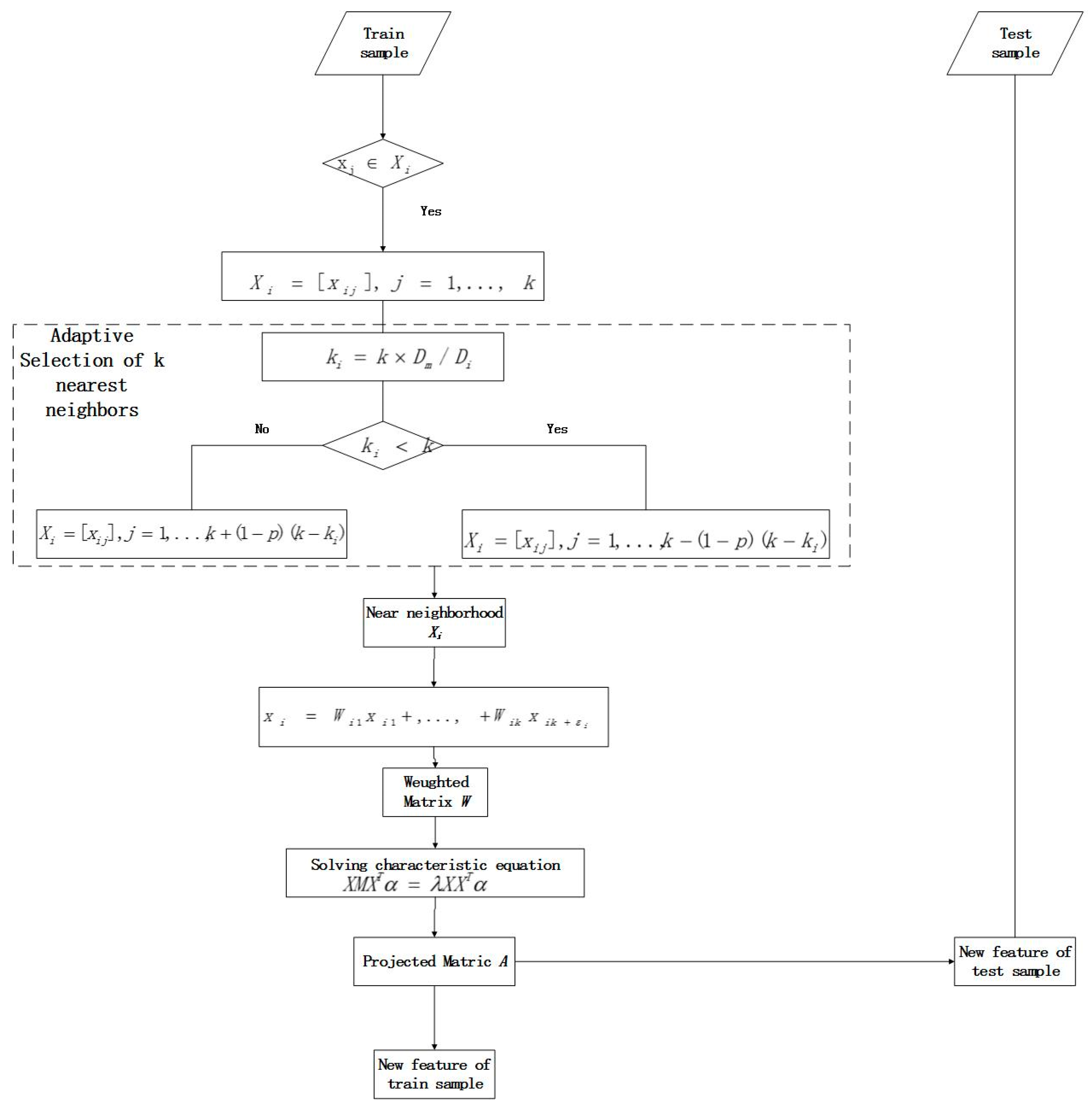
3.1. ANSNPE Algorithm

The Neighborhoods Preserving Embedding (NPE) algorithm is a linear approximation of the LLE algorithm aimed at preserving the local manifold structure of data. The premise is that in a local domain, a point can be represented linearly by the points around it. The objective is for the weight coefficients of the linear representation of the adjacent sample points in the original data space to remain consistent in the projected space [14]. Assuming that a training sample is represented by a high-dimensional feature set $\mathit{X}=\left[x_1,\dots ,x_n\right]\in R^{m\times n}$, m is the characteristic number, which is the space dimension, and n is the sample number. The intrinsic characteristic of the sample is the low-dimensional manifold structure embedded in the m dimensional space. The low-dimensional feature of the output is represented as $\mathit{Y}=\left[y_1,\dots ,y_n\right]\in R^{d\times n}(d<m)$. The major steps are as follows:

• Finding the k nearest neighbors of the sample X_i, the affine reconstruction of X_i is performed by these neighborhood points. To minimize the reconstruction error, the optimized objective function is designed as the following Equation (1);

  $$\mathrm{argmin}{\Vert {\epsilon }_i\Vert }^2=argmin{\displaystyle \sum }_i\Vert X_i-{\displaystyle \sum }_i{W}_{ij}{X}_j{\Vert }^2{\displaystyle \sum }_j{W}_{ij=1,j=1,2,\dots ,n}$$

  (1)
• Calculating the weight matrix W according to the optimized objective function;
• Solving the characteristic equation; the characteristic vectors corresponding to the d smallest eigenvalues of the equation is the projection matrix of A($A\in R^{d\times m}$);
• New features of the training image are obtained by the feature mapping of training samples by the projection matrix.

In the NPE algorithm, any sample point is represented by the linear reconstruction of its k neighbor point, and the other points in the k nearest neighbor point can be reconstructed linearly by the k-1 points. If the value of k is selected reasonably [51], the linear reconstruction error will be very close. However, if the value of k is not reasonable, the linear reconstruction error will be larger. In practical applications, the distribution density of data is generally different, and the number of corresponding neighbor points should also be changed [52]. In the NPE algorithm, it is easy to have a large reconstruction error when the fixed value of k is set for every point. Therefore, an adaptive neighborhood selection neighborhood preserving embedding (ANSNPE) algorithm is proposed by introducing the adaptive neighborhood selection method. The algorithm is shown in Figure 1, and the major steps are as follows:

• The initial neighbor parameter k, the minimum neighbor point parameter k_min, the maximum neighbor point parameter k_max, and the small event selection probability p are set. Finding the initial k nearest neighbors of samples X_i (X_i = [x_ij], j = 1, …, k);
• Selecting the k nearest to the neighbors adaptively. The mean Euclidean distance D_i and the mean manifold distance D_m of the sample point X_i are calculated to obtain the parameter k_i of sample X_i by D_i and D_m (e.g., Equations (2)–(4)). If k_i < k, it means that the D_i is larger and the neighbor data of X_i is sparse; then, it is necessary to eliminate the larger (1 − p) (k − k_i) [53] Euclidean distance in the data set. If k_i > k, it means that the D_i is smaller and that the data are more dense. At the same time, it retains X_i as the neighborhood data, and the rest (1 − p)(k − k_i) of the Euclidean distance smaller points are selected to join the neighborhood X_i;
• Obtain the final neighbor of X_i and calculate the weight matrix W according to the optimized objective function;
• Solving the characteristic equation; the characteristic vectors corresponding to the d smallest eigenvalues of the equation is the projection matrix of A($A\in R^{d\times m}$); and
• New features of the training image are obtained using the feature mapping of training samples by the projection matrix.

  $$D_i=\frac{{{\displaystyle \sum }}_{j=1}^k{\mathit{X}}_{\mathrm{i}}-{\mathit{X}}_{ij}}{k},i=1,2,\dots ,n$$

  (2)

  $$D_m=\frac{{{\displaystyle \sum }}_{i=1}^n{D}_i}{n}$$

  (3)

  $$k_i=k\times \frac{D_m}{D_i}$$

  (4)

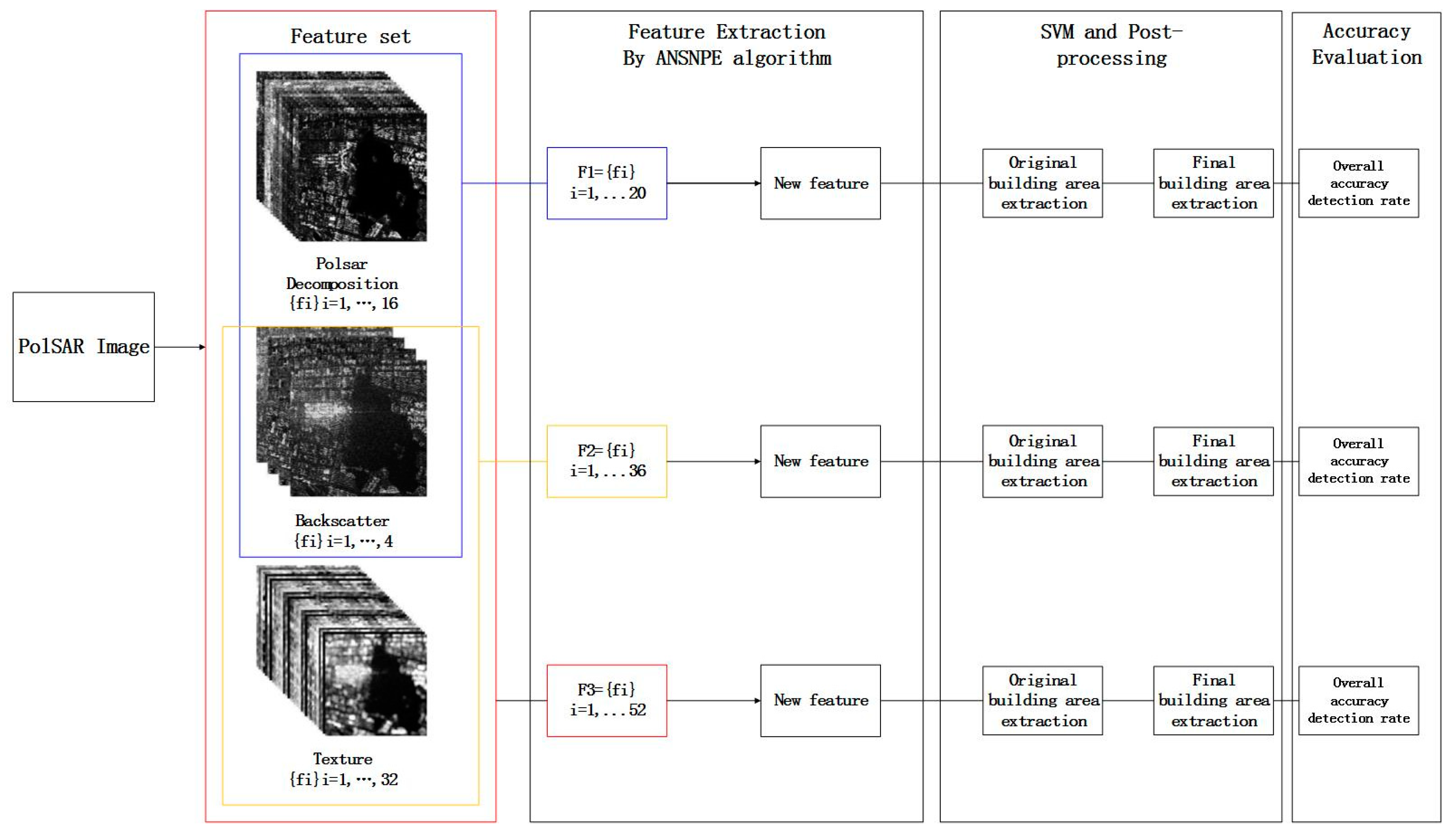
3.2. Extraction Framework

The three categories of features and their combination can be written as three feature sets, which are F1 = {f_i}_i=1,…,20, F2 = {f_i}_i=1,…,36, F3 = {f_i}_i=1,…,52, and the procedure is shown in Figure 2. ANSNPE is applied to the three feature sets to extract new features. Then, new features are as an input of the SVM classier to obtain preliminary construction area extraction results. Finally, the final extracted construction area is obtained by the post processing of the preliminary results.

4. Experiments and Results

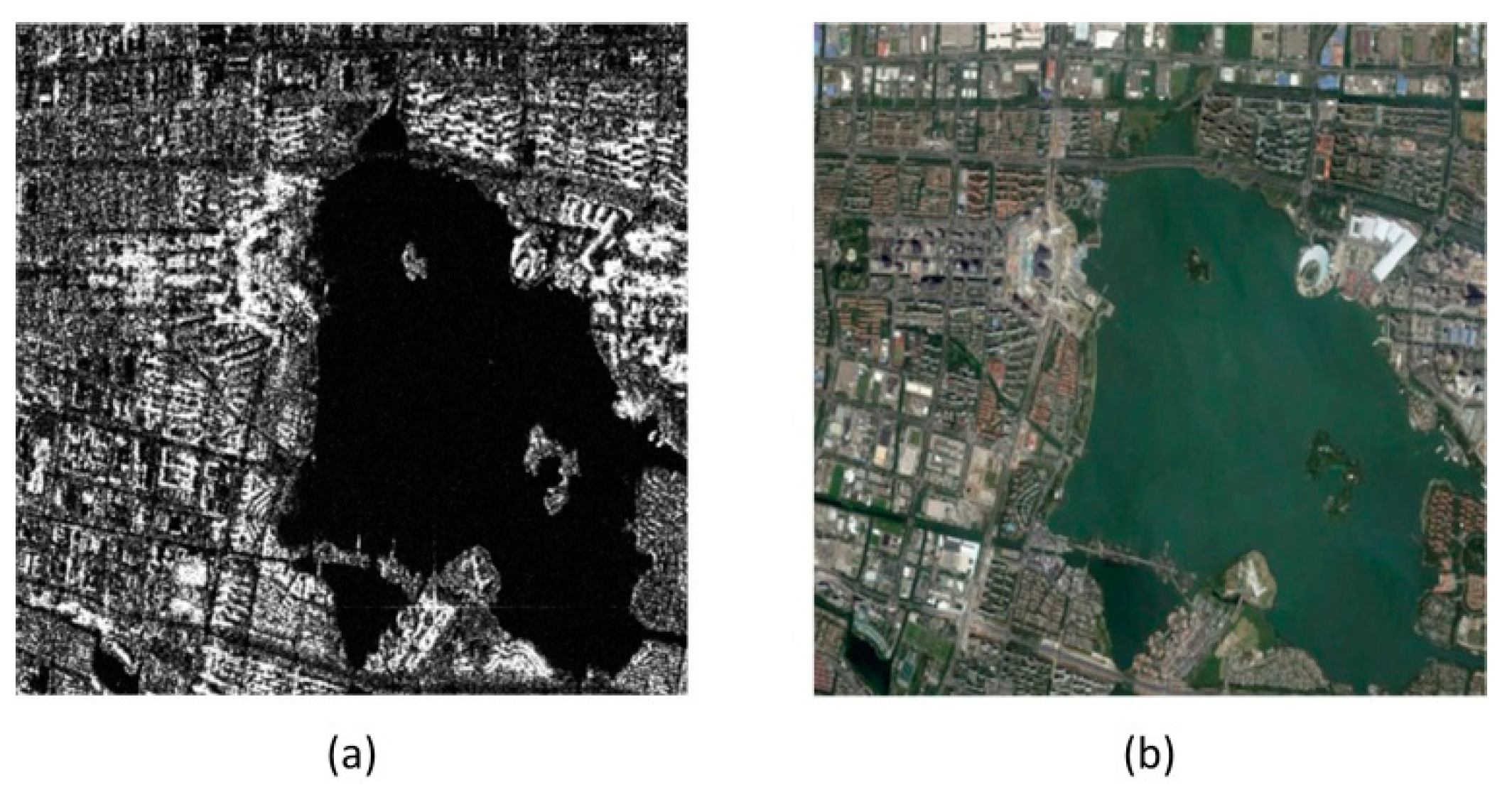
In this section, there are four experiments. One is that we discuss the selection of parameter d by using various d to obtain the extraction accuracy. In the second experiment of building extraction, the proposed method is compared with the original dimension-reduced method NPE, with linear dimensionality reduction principal component analysis (PCA), and with no dimensionality reduction. For the three data sets, the four approaches are applied. The overall accuracy (OA) are used to evaluate the performance of the different methods. In the third experiment, we discuss the applicability analysis of ANSNPE, which is the influence of selecting training samples. In the last experiment, we choose GF3 data as experiment data to demonstrate the applicability of the proposed method to different data sources.

4.1. Data

RADARSAT-2 and GF3 images of Suzhou are obtained from a subset of C-band, PolSAR data, which was acquired in 2017. Detailed information of RADARSAT and GF3 is listed in

Table 4. The Parameters of RADARSAT-2 and GF3.

Parameters	RADARSAT-2	GF3
Resolution	6.17 m	8.00 m
Direction	Ascending	Descending
Imaging Mode	Fine Quad-Pol	QPSI
Incidence Angle	4.01–4.05	29.68–31.42
Time	2017.07.17	2017.01.29

. Figure 3a shows the amplitude image of RADARSAT-2, Figure 3b shows the corresponding Google Earth image. The size of the image is 800 × 800.

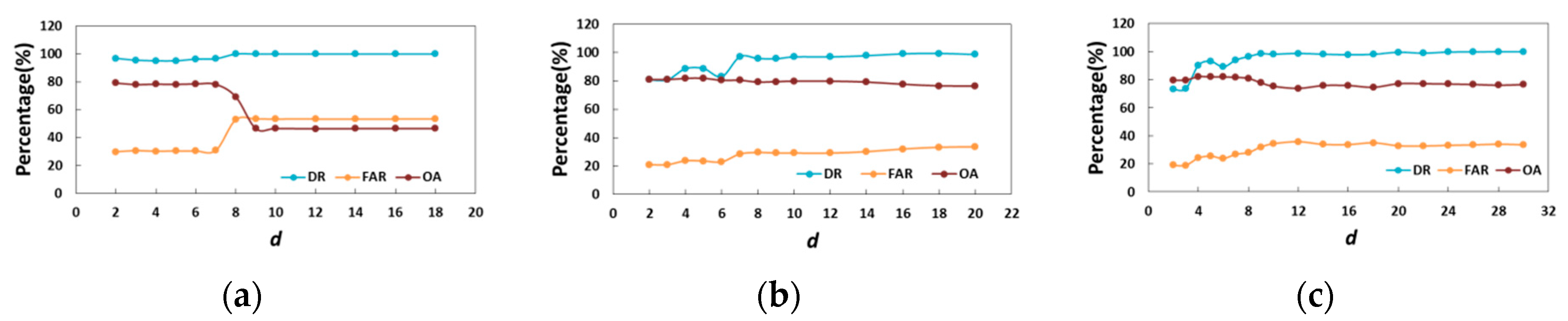
4.2. Discussion of the Parameter d

The estimation of intrinsic dimensionality is a problem. There is no approach to confirm it (Tu et al., 2010). In this paper, parameter d is determined through experiments. Figure 3 shows the extraction accuracy under various choices of d. In Figure 4, blue refers to the detection rate (DR), red refers to the overall accuracy (OA), and orange refers to the false alarm rate (FAR). The range of d is from 2 to 20 for F1 and F2 and from 2 to 20 for F3. As shown in Figure 3, for the F1 dataset, OA has the best performance when d is in the value of 2 to 7. FAR keeps stable since d is 4. Moreover, the processing time is longer when the d is higher. Consequently, the parameter d for F1 is set as 4. For the F2 dataset, d in the value of 4 has the best performance. For the F3 dataset, d in the value of 8 has the best performance. Therefore, d is respectively set as 4, 4, and 8 in the experiments for F1, F2, and F3.

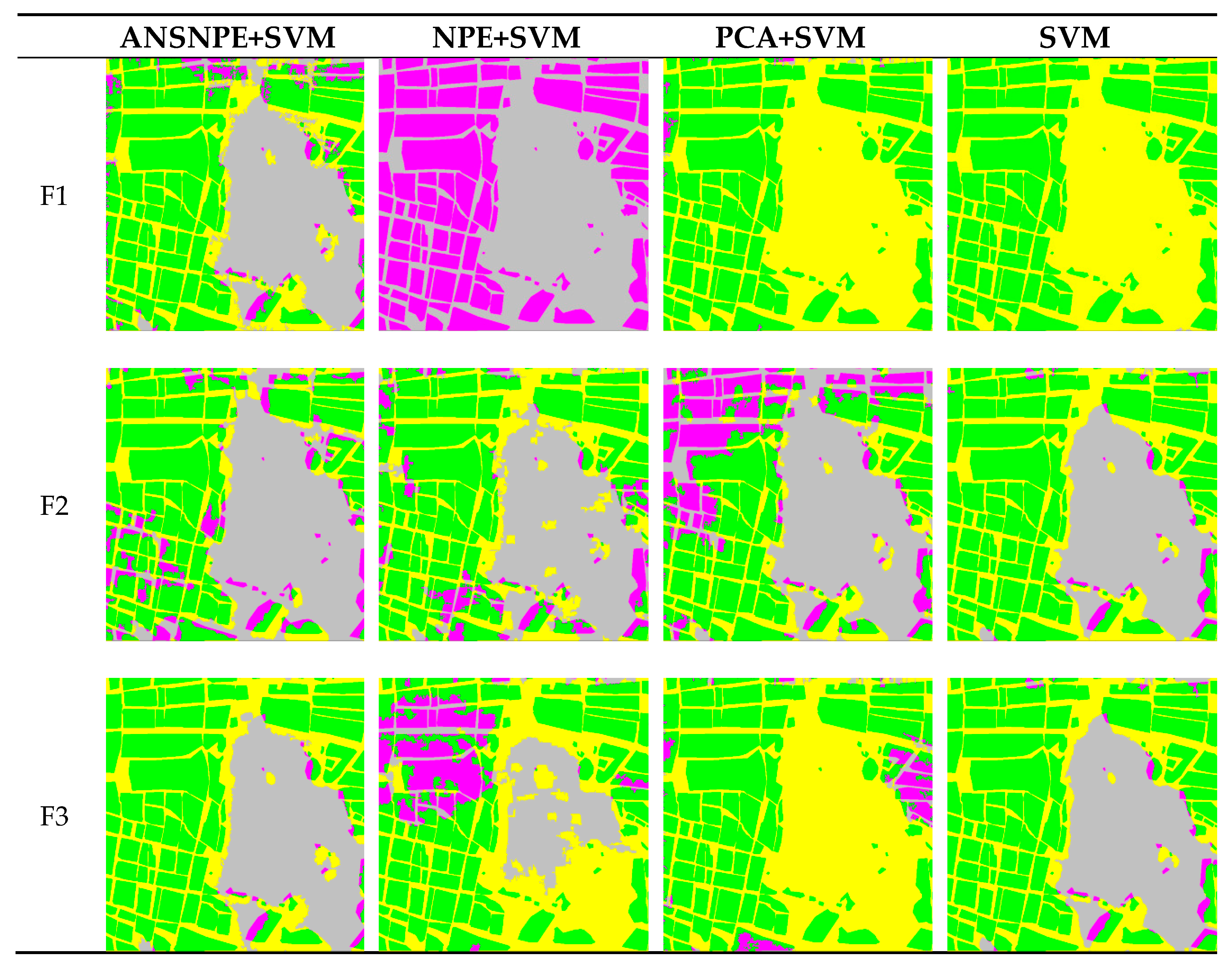
4.3. Experiments of Building Extraction

In this section, RADARSAT-2 image is used to evaluate the proposed algorithm. A total of 6400 training samples are selected from subset of RADARSAT-2 to extract features and obtain the project matrix. For comparative experiments, the other extracted methods use the same training samples. For the ANSNPE algorithm, the parameter k is set as 15, where k_min is 1, k_max is 30, and p is 0.3. Figure 5, Figure 6 and Figure 7 shows the final building area extracted results of all methods. The extraction results are compared with the true values obtained from the visual interpretation of optical images.

Table 5. Extraction accuracy of the three feature sets.

Feature Set	Evaluation	ANSNPE+SVM(%)	NPE+SVM(%)	PCA+SVM(%)	SVM(%)
F1	IDR	74.97	3.27	75.58	95.32
	IOA	74.03	54.71	36.45	68.35
	DR	95.23	0	99.55	100
	OA	78.09	53.47	46.34	46.59
F2	IDR	87.79	80.32	70.43	95.55
	IOA	81.94	69.92	75.38	76.77
	DR	88.78	89.43	73.23	99.07
	OA	81.88	73.69	75.28	77.75
F3	IDR	94.56	70.39	55.38	95.84
	IOA	81.42	50.04	29.74	76.77
	DR	96.42	76.56	92.02	99.17
	OA	80.89	50.94	43.64	77.76

gives the initial detection rate (IDR), the initial overall accuracy (IOA), the final detection rate (DR) and overall accuracy (OA) of the extracted results.

The DR and OA of F1+ANSNPE+SVM are 95.23% and 78.09%, and those of F1+SVM are 100% and 46.59%. The DR and OA of F2+ANSNPE+SVM are 88.78% and 81.88%, and those of F2+SVM are 99.07% and 77.75%. The DR and OA of F3+ANSNPE+SVM are 96.42% and 80.89%, and those of F3+SVM are 99.17% and 77.76%. The best results are in bold in Table 5. It shows that the precision of the building area extraction by the ANSNPE algorithm is higher than that of the building area directly extracted by original features.

For the F1 dataset, the performance of building area extraction by the ANSNPE algorithm is much better than one of other algorithms. The building area is not extracted by the NPE algorithm. The other two algorithms extracted about 40 percent of building area, which is water area. It illustrates that the three algorithms fail to find and preserve the intrinsic pattern structure of the SAR image. In the experiment in the F2 dataset, the result of ANSNPE is better. More building area, especially the low building area, is not be extracted by the NPE and PCA algorithm. For the F3 dataset, the same phenomenon appears. The OA of SVM, which has no feature extraction, is higher than NPE and PCA, however, it is lower than the proposed ANSNPE algorithm.

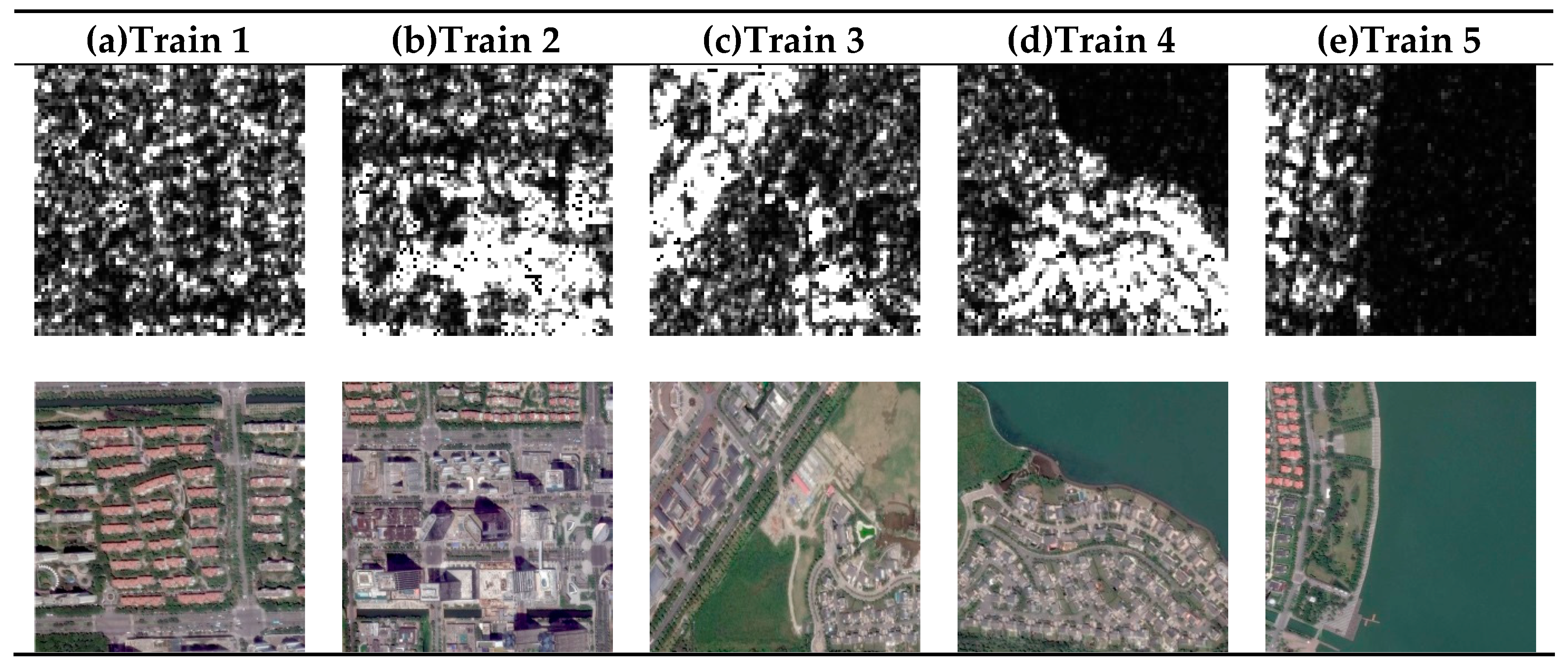
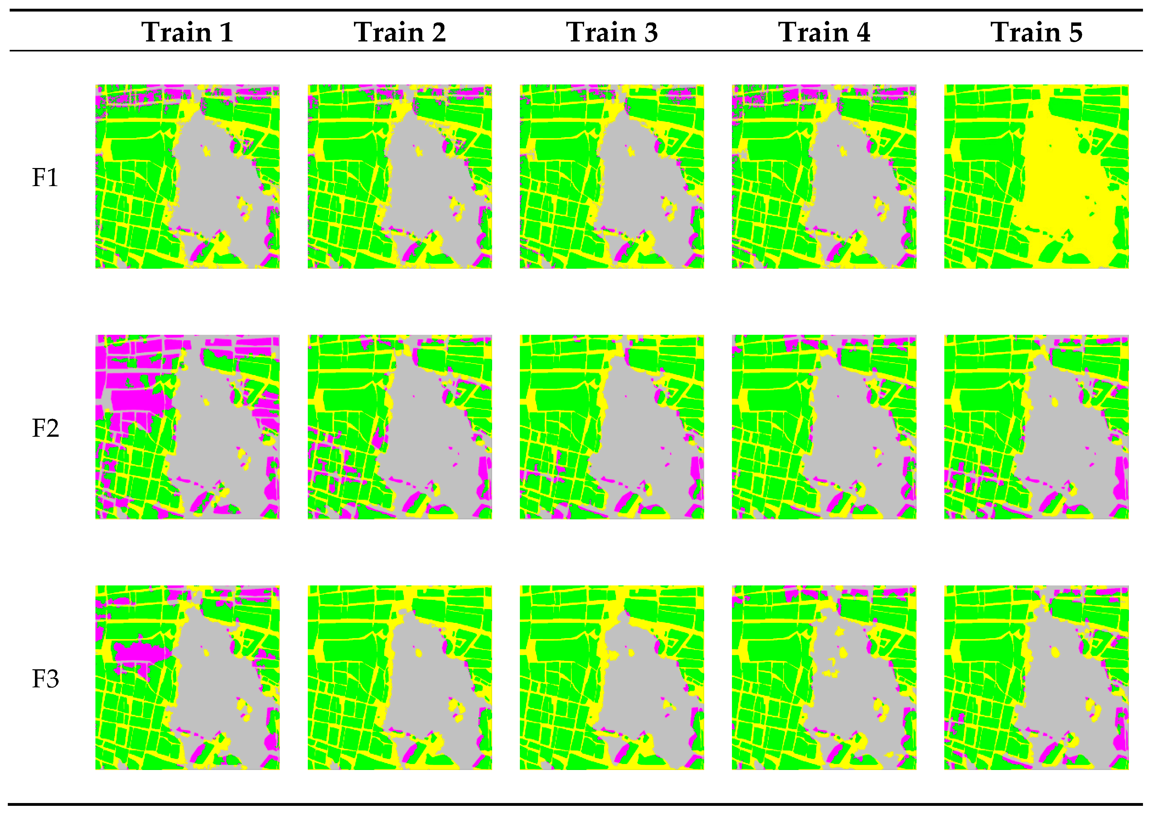
4.4. Applicability Analysis

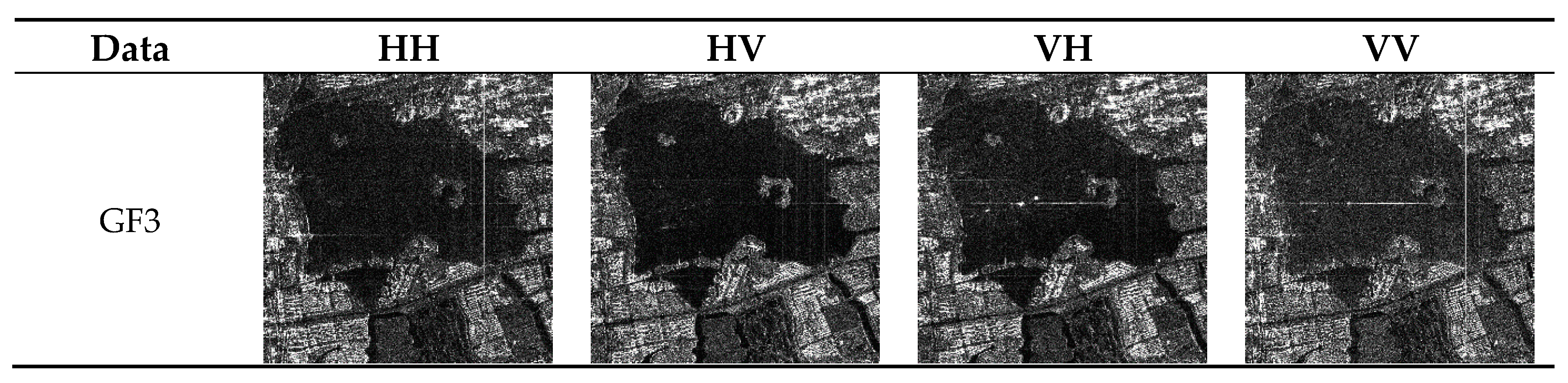
Because of the generalization of the ANSNPE algorithm, the selection of training samples may be affected by the results of test samples by generating features that cannot distinguish the building area. Therefore, depending on the type of ground objects, five training samples with different combinations of building areas, vegetation, and water are selected for study in Figure 6. The project matrix is applied to the test image, and the results are shown in Figure 7 and

Table 6. Extraction accuracy of three feature sets.

Feature Set		Train 1 (%)	Train 2 (%)	Train 3 (%)	Train 4 (%)	Train 5 (%)	Average (%)	Standard Deviation
F1	IDR	70.8	74.97	76.68	71.17	93.27	77.38	8.25
	IOA	72.62	74.03	74.2	73.33	68.06	72.45	2.26
	DR	91.52	95.23	96.78	92.51	99.99	95.21	3.04
	OA	77.27	78.09	77.63	77.51	46.61	71.42	12.41
F2	IDR	46.83	87.79	92.31	87.22	88.92	80.61	16.98
	IOA	67.62	81.94	80.99	80.45	81.73	78.55	5.49
	DR	51.39	88.78	92.96	93.68	90.59	83.48	16.13
	OA	68.65	81.88	80.51	81.35	81.72	78.82	5.11
F3	IDR	75.35	94.56	99.43	92.72	90.76	90.56	8.13
	IOA	71.69	81.42	76.52	78.01	80.46	77.62	3.44
	DR	82.66	96.42	99.57	96.16	93.49	93.66	5.83
	OA	73.69	80.89	76.53	78.66	80.47	78.05	2.67

. The best results are in bold. The average accuracy of F1+ANSNPE+SVM is 71.42%, and the standard deviation is 12.41; the average accuracy of F2+ANSNPE+SVM is 78.82%, and the standard deviation is 5.11; and the average accuracy of F3+ANSNPE+SVM is 78.05%, and the standard deviation is 2.67.

There are some differences observed among the OA of F1+ANSNPE+SVM, F2+ANSNPE+SVM, and F3+ANSNPE+SVM. The OA of F1 is lower, and the reason for this result is that some water is falsely detected as the building area. F2 and F3 had a close OA, but the DR of F3 is more than 95% and is 8% more than that of F2. Some building areas are not detected in F2. Undetected building areas are mainly concentrated where buildings are relatively low, and the texture features are not obvious. In the three experiments, the error is mainly caused by the road construction area because the effect of the top displacement of high buildings makes the brightness extend to the road, and then the classifier mistakenly identifies the road as a building area.

In the applicability analysis, different training samples are applied to the test image, and the accuracy of building area extraction is different. The average OA of F1 is lower and fluctuated greatly; only the feature set composed of polarization features is used to extract the building area to obtain low accuracy, and the information it provided is not enough. In the F2 experiments, when the training sample is train 1, the OA is lowest. As a result, the building in train 1 is low, and the texture feature is not obvious. The extracted projection matrix is applied to the high-dimensional feature set composed of texture features, which cannot be used to extract good features for the building area. However, the average OA of F3 is not much different from that of F2, and the fluctuated value is lower.

4.5. GF3 Data

The proposed method is applied on the GF3 data. Figure 8 shows the backscattering image of GF3. Figure 9 and

Table 7. Extraction Accuracy of GF3 data.

Evaluation	F1 (%)	F2 (%)	F3 (%)
IDR	68.95	66.56	75.29
IOA	87.53	87.5	88.18
DR	69.36	65.93	74.14
OA	88.32	87.24	88.32

give extracted results. In Figure 8, F3 has a better performance than F1 and F2. As can be seen from Table 7, the highest OA obtained by the proposed method with F3 and F1 is 88.32%. The highest DR is 74.14%, which is respectively about 4% and 8% higher than F1 and F2.

As shown in Figure 8, the top displacement of the building happens in the horizontal and vertical polarization images, which influences the results of F1. The non-building area is extracted as the building area. However, there are not false extracted building areas in the results of F2 at the same place. In addition, F3 can extract the building area, which is missed with F1 and F2. For GF3, all features, including the polarization feature and texture feature, are better chosen to extract building area.

5. Conclusions

PolSAR images have characteristics of high dimensions and nonlinearity. Embedding high-dimensional SAR data in high-dimensional space and describing the intrinsic geometric structure of SAR data can improve the accuracy of SAR information extraction. Therefore, it is of important theoretical and practical value to study the method of building area extraction from high-resolution PolSAR images. This paper analyzed the principle of the NPE algorithm and proposes a building area extraction method using high-resolution PolSAR images based on the ANSNPE algorithm. First, we used the gray engineering matrix and various polarization decomposition methods to make up the high-dimensional collection, consisting of 20, 36, and 52, respectively. Next, a low-dimensional projection matrix is obtained using the ANSNPE algorithm, and the high-dimensional features are reduced. Lastly, the SVM classification method is used to extract the building area and the detection rate, and the overall accuracy is calculated. Through a contrast test, it was found that the accuracy of building area extraction based on the ANSNPE algorithm is over 80%, which is higher than that obtained when using the original high-dimensional feature extraction. Through the applicability analysis, it is found that different training samples affect the accuracy of building area extraction and that polarization decomposition features provide rich information, complementary to texture features, and can extract the features that are beneficial to the extraction of building areas. Experiments on GF3 data verify that the proposed method is also applicable and that it is better to choose all features when building an area extraction with GF3. However, there are some non-extracted building areas. The next step will be to study how to reduce the accuracy of error extraction, considering the application of the better ANSNPE algorithm on the bigger area. Moreover, our aim is also to extract buildings more accurately and more rapidly.

References

1. Xu, J. Urban Change Detection from Space borne PolSAR Images with Radiometric Corrections. Ph.D. Thesis, Wuhan University, Wuhan, China, 2015. [Google Scholar]
2. Luo, D. Fusion of High Spatial Resolution Optical and Polarimetric SAR Images for Urban Land Cover Classification. Master’s Thesis, Chongqing Jiaotong University, Chongqing, China, 2015. [Google Scholar]
3. Tan, Q.L.; Shao, Y. A Study on the Development of New Classification Technology for Radar Remote Sensing Imagery. Remote Sens. Land Resour. 2001, 49, 1–7. [Google Scholar] [CrossRef]
4. Zhao, L.J.; Gao, G.; Kuang, G.Y. Variogram-based Build-up Areas Extraction from High-resolution SAR Images. Signal Process. 2009, 25, 1433–1442. [Google Scholar] [CrossRef]
5. Zhu, J.H.; Guo, H.D.; Fan, X.T.; Zhu, B.Q. The Application of the Wavelet Texture Method to the Classification of Single-Band, Single-Polarized and High-resolution Sar Images. Remote Sens. Land Resour. 2005, 64, 36–39. [Google Scholar] [CrossRef]
6. Zhao, L.J.; Qin, Y.L.; Gao, G.; Kuang, G.Y. Detection of built-up areas from High-Resolution SAR Images Using GLCM textural analysis. J. Remote Sens. 2009, 13, 483–490. [Google Scholar] [CrossRef]
7. Shang, T.T.; Jia, Y.C.; Wen, Y.; Sun, H. Laplacian Eigenmaps-Based Polarimetric Dimensionality Reduction for SAR Image Classification. IEEE Trans. Geosci. Remote Sens. 2012, 50, 170–178. [Google Scholar] [CrossRef]
8. Huang, Q.; Liu, H. Overview of Nonlinear Dimensionality Reduction Methods in Manifold Learning. Appl. Res. Comput. 2007, 24, 19–25. [Google Scholar] [CrossRef]
9. Tenenbaum, J.B.; Silva, V.; Langford, J.C. A Global Geometric Framework for Nonlinear Dimensionality Reduction. Science 2000, 290, 2319–2323. [Google Scholar] [CrossRef]
10. Roweis, S.T.; Saul, L.K. Nonlinear dimensionality reduction by locally linear embedding. Science 2000, 290, 2323–2326. [Google Scholar] [CrossRef] [PubMed] [Green Version]
11. Belkin, M.; Niyogi, P. Laplacian eigenmaps for dimensionality reduction and data representation. Neural Comput. 2003, 15, 1373–1396. [Google Scholar] [CrossRef] [Green Version]
12. Zhang, Z.; Zha, H.Y. Principal Manifolds and Nonlinear Dimension Reduction via Local Tangent Space Alignment.SIAM. J. Sci. Comput. 2005, 26, 313–338. [Google Scholar] [CrossRef] [Green Version]
13. He, X.; Niyogi, P. Locality Preserving Projections. Neural Inf. Process. Syst. 2004, 16, 153–160. [Google Scholar]
14. He, X.; Cai, D.; Yan, S.; Zhang, H.J. Neighborhood Preserving Embedding. In Proceedings of the Tenth IEEE International Conference on Computer Vision, Beijing, China, 17–20 October 2005; Volume 2, pp. 1208–1213. [Google Scholar]
15. Xia, J.S.; Bombrun, L.; Berthoumieu, Y.; Germain, C. Multiple features learning via rotation strategy. In Proceedings of the International Conference on Image Processing (ICIP), Phoenix, AZ, USA, 25–28 September 2016. [Google Scholar] [CrossRef]
16. Chang, C.S.; Chen, K.C.; Kuo, B.C.; Wang, M.S.; Li, C.H. Semi-supervised local discriminant analysis with nearest neighbors for hyperspectral image classification. In Proceedings of the Geoscience and Remote Sensing Symposium, Quebec City, QC, Canada, 13–18 June 2014. [Google Scholar] [CrossRef]
17. Xia, J.S.; Chanussot, J.; Du, P.J.; He, X. Spectral–Spatial Classification for Hyperspectral Data Using Rotation Forests With Local Feature Extraction and Markov Random Fields. IEEE Trans. Geosci. Remote Sens. 2015, 53, 2532–2546. [Google Scholar] [CrossRef]
18. Liao, W.Z.; Pizurica, A.; Philips, W.; Pi, Y. Feature extraction for hyperspectral images based on semi-supervised local discriminant analysis. In Proceedings of the 2011 Joint Urban Remote Sensing Event, Munich, Germany, 11–13 April 2011. [Google Scholar] [CrossRef]
19. Watanabe, K. Coherency Preserving Feature Transformation for Semantic Segmentation. In Proceedings of the 2018 IEEE International Conference on Systems, Man, and Cybernetics (SMC), Miyazaki, Japan, 7–10 October 2018; pp. 1368–1373. [Google Scholar] [CrossRef]
20. Zhang, H.S.; Li, J.; Wang, T.; Lin, H.; Zheng, Z.; Li, Y.; Lu, Y. A manifold learning approach to urban land cover classifification with opticalandradar dat. Landsc. Urban Plan. 2018, 172, 11–24. [Google Scholar] [CrossRef]
21. Lou, J.; Jin, T.; Zhou, Z.M. Feature extraction for landmine detection in uwb sar via swd and isomap. Prog. Electromagn. Res. 2013, 138, 157–171. [Google Scholar] [CrossRef] [Green Version]
22. Li, B.; Gong, J.B.; Tian, J.W. Selection of matching area in sar scene-matching-aided navigation based on manifold learning. In Proceedings of the Seventh International Symposium on Multispectral Image Processing and Pattern Recognition (MIPPR2011), Guilin, China, 4–6 November 2011. [Google Scholar] [CrossRef]
23. Chen, B.; Cao, Y.F.; Sun, H. Active sample-selecting and manifold learning-based relevance feedback method for synthetic aperture radar image retrieval. IET Radar Sonar Navig. 2011, 5, 118–127. [Google Scholar] [CrossRef]
24. Shi, L.; Zhang, L.F.; Yang, J.; Zhang, L.; Li, P. Supervised Graph Embedding for Polarimetric SAR Image Classification. IEEE Geosci. Remote Sens. Lett. 2013, 10, 216–220. [Google Scholar] [CrossRef]
25. Dong, G.G.; Kuang, G.Y. Target recognition in sar images via classification on riemannian manifolds. IEEE Geosci. Remote Sens. Lett. 2015, 12, 199–203. [Google Scholar] [CrossRef]
26. Shi, L.; Zhang, L.F.; Zhao, L.L.; Zhang, L.; Li, P.; Wu, D. Adaptive laplacian eigenmap-based dimension reduction for ocean target discrimination. IEEE Geosci. Remote Sens. Lett. 2016, 13, 902–906. [Google Scholar] [CrossRef]
27. Cao, H.; Zhang, H.; Wang, C. Supervised locally linear embedding for polarimetric sar image classification. In Proceedings of the 2016 IEEE International Geoscience and Remote Sensing Symposium (IGARSS), Fort Worth, TX, USA, 10–15 July 2016; pp. 7561–7564. [Google Scholar] [CrossRef]
28. Yu, M.; Zhang, S.Q.; Dong, G.G. Target recognition in sar image based on robust locality discriminant projection. IET Radar Sonar Navig. 2018, 12, 1285–1293. [Google Scholar] [CrossRef]
29. Hu, J.L.; Hong, D.F.; Wang, Y.Y. A comparative review of manifold learning techniques for hyperspectral and polarimetric sar image fusion. Remote Sens. 2019, 11, 681. [Google Scholar] [CrossRef] [Green Version]
30. Wang, H.J.; Han, J.H.; Deng, Y.Y. Polsar image classification based on laplacian eigenmaps and superpixels. Eurasip J. Wirel. Commun. Netw. 2017, 2017, 198. [Google Scholar] [CrossRef] [Green Version]
31. Wang, J.; Sun, L.Z. Research on supervised manifold learning for sar target classification. In Proceedings of the CIMSA 2009—International Conference on Computational Intelligence for Measurement Systems and Applications, Hong Kong, China, 11–13 May 2009. [Google Scholar] [CrossRef]
32. Li, T. Method Research of Recognition of Urban Building Areas from High Resolution SAR Images Based on Manifold Learning. Master’s Thesis, University of Chinese Academy of Sciences, Beijing, China, 2015. [Google Scholar]
33. Miao, A.M.; Ge, Z.Q.; Song, Z.H.; Shen, F. Nonlocal structure constrained neighborhood preserving embedding model and its application for fault detection. Chemom. Intell. Lab. Syst. 2015, 142, 184–196. [Google Scholar] [CrossRef]
34. Miao, A.M.; Li, P.; Ye, L. Neighborhood preserving regression embedding based data regression and its applications on soft sensor modeling. Chemom. Intell. Lab. Syst. 2015, 147, 86–94. [Google Scholar] [CrossRef]
35. Miao, S.; Wang, J.; Gao, Q.X.; Chen, F.; Wang, Y. Discriminant structure embedding for image recognition. Neurocomputing 2016, 174, 850–857. [Google Scholar] [CrossRef]
36. Chen, L.; Li, Y.J.; Li, H.B. Facial expression recognition based on image Euclidean distance-supervised neighborhood preserving embedding. In Proceedings of the International Symposium on Optoelectronic Technology and Application 2014: Image Processing and Pattern Recognition, Beijing, China, 13–15 May 2014. [Google Scholar] [CrossRef]
37. Zhang, S.H.; Li, W.H. Bearing Condition Recognition and Degradation Assessment under Varying Running Conditions Using NPE and SOM. Hindawi Publ. Corp. Math. Probl. Eng. 2014, 781583. [Google Scholar] [CrossRef]
38. Pang, M.; Jiang, J.F.; Lin, C.; Wang, B. Two dimensional discriminant neighborhood preserving embedding in face recognition. In Proceedings of the Sixth International Conference on Graphic and Image Processing, Beijing, China, 24–26 October 2014. [Google Scholar] [CrossRef]
39. Liu, X.M.; Yin, J.W.; Feng, Z.L.; Dong, L.; Wang, L. Orthogonal Neighborhood Preserving Embedding for Face Recognition. In Proceedings of the 2007 IEEE International Conference on Image Processing, San Antonio, TX, USA, 16–19 September 2007; pp. 1522–4880. [Google Scholar] [CrossRef]
40. Wang, N.; Li, X. Face Clustering Using Semi-supervised Neighborhood Preserving Embedding with Pairwise Constraints. In Proceedings of the 2009 4th IEEE Conference on Industrial Electronics and Application, Xi’an, China, 25–27 May 2009; pp. 2156–2318. [Google Scholar] [CrossRef]
41. Tao, X.; Dong, S.F.; Zhao, Q.X.; Han, Z. Kernel Neighborhood Preserving Embedding and its Essence Analysis. In Proceedings of the 2009 WRI Global Congress on Intelligent Systems, Xiamen, China, 19–21 May 2009; pp. 2155–6083. [Google Scholar] [CrossRef]
42. Lai, Z. Sparse local discriminant projections for discriminant knowledge extraction and classification. IET Comput. Vis. 2012, 6, 551–559. [Google Scholar] [CrossRef]
43. BAO, X.; Zhang, L.; Wang, B.J.; Yang, J. A Supervised Neighborhood Preserving Embedding for Face Recognition. In Proceedings of the International Joint Conference on Neural Networks (IJCNN), Beijing China, 6–11 July 2014. [Google Scholar] [CrossRef]
44. Wen, J.H.; Yan, W.D.; Lin, W. Supervised Linear Manifold Learning Feature Extraction for Hyperspectral Image Classification. In Proceedings of the Geoscience and Remote Sensing Symposium, Quebec City, QC, Canada, 13–18 July 2014. [Google Scholar] [CrossRef]
45. Yuan, X.F.; Ge, Z.Q.; Ye, L.J.; Song, Z. Supervised neighborhood preserving embedding for feature extraction and its application for soft sensor modeling. J. Chemom. 2016, 30, 430–441. [Google Scholar] [CrossRef]
46. Ran, R.S.; Fang, B.; Wu, X.G. Exponential Neighborhood Preserving Embedding for Face Recognition. IEICE Trans. Inf. Syst. 2018, 101, 1410–1420. [Google Scholar] [CrossRef] [Green Version]
47. Mehta, S.; Zhan, B.S.; Shen, X.J. Weighted Neighborhood Preserving Ensemble Embedding. Electronics 2019, 8, 219. [Google Scholar] [CrossRef] [Green Version]
48. Wang, X.Y.; Cao, Z.J.; Cui, Z.Y.; Liu, N.; Pi, Y. PolSAR image classification based on deep polarimetric feature and contextual information. J. Appl. Remote Sens. 2019, 2019, 13. [Google Scholar] [CrossRef]
49. Harakck, R.M.; Shanmugam, K.; Dinstein, I.H. Textural Features for Image Classification. Trans. Syst. Man Cybern. 1973, 3, 610–621. [Google Scholar] [CrossRef] [Green Version]
50. Jong-Sen, L.; Eric, P. Polarimetric Radar Imaging: From Basics to Applications; Publishing House of Electronics Industry: Beijing, China, 2013; pp. 134–168. ISBN 978-7-121-20266-7. [Google Scholar]
51. Hui, K.H.; Xiao, B.H.; Wang, C.H. Self-Regulation of Neighborhood Parameter for Locally Linear Embedding. Pattern Recognit. Artif. Intell. 2010, 23, 842–846. [Google Scholar] [CrossRef]
52. Huang, L.Z.; Zheng, L.X.; Chen, C.Y.; Min, L. Locally Linear Embedding Algorithm with Adaptive Neighbors. In Proceedings of the International Workshop on Intelligent Systems and Applications, Wuhan, China, 23–24 May 2009; pp. 1–4. [Google Scholar] [CrossRef]
53. Zhang, Y.L.; Zhuang, J.; Wang, N.; Wang, S.A. Fusion of Adaptive Local Linear Embedding and Spectral Clustering Algorithm with Application to Fault Diagnosis. J. Xi’an Jiaotong Univ. 2010, 44, 77–82. [Google Scholar] [CrossRef]
Figure 1. The flowchart of the Adaptive Neighborhoods selection Neighborhood Preserving Embedding (ANSNPE) algorithm.
Ijgi 09 00109 g001
Figure 2. The Extraction Framework.
Ijgi 09 00109 g002
Figure 3. (a) The RADARSAT-2 and (b) the corresponding Google Earth image.
Ijgi 09 00109 g003
Figure 4. Discussion of the d experiment, (a) is the result of F1 dataset, (b)is F2 dataset, (c)is F3 dataset.
Ijgi 09 00109 g004
Figure 5. Classification results of three feature sets. Yellow means incorrect building areas, which are extracted; green shows the properly extracted building areas; red shows the building areas not being extracted; and gray shows the non-built areas.
Ijgi 09 00109 g005
Figure 6. Train area and corresponding Google images. (a) Train 1: low buildings; (b) train 2: high buildings; (c) train 3: buildings and plants; (d) train 4: buildings, plants, and water; (e) train 5: building, plant, and water.
Ijgi 09 00109 g006
Figure 7. Classification results of the three feature sets. Yellow shows the incorrect building areas, which are extracted; green shows the properly extracted building areas; red shows the building areas not being extracted; and gray shows the non-built areas.
Ijgi 09 00109 g007
Figure 8. Backscattering characteristics of GF3.
Ijgi 09 00109 g008
Figure 9. Extraction of GF3 with three feature sets. (a) F1 +ANSNPE+SVM (b) F2+ANSNPE+SVM (c) F3+ANSNPE+SVM. Yellow shows the incorrect building areas, which are extracted; green shows the properly extracted building areas; red shows the building areas not being extracted; and gray shows the non-built areas.
Ijgi 09 00109 g009