Article

A High-Resolution Spatial and Time-Series Labeled Unmanned Aerial Vehicle Image Dataset for Middle-Season Rice

1
National Engineering Laboratory for Educational Big Data, Central China Normal University, 152 Luoyu Road, Wuhan 430079, China
2
National Engineering Research Center for E-Learning, Central China Normal University, 152 Luoyu Road, Wuhan 430079, China
3
Sichuan Branch, China Construction Bank Corporation, 86 Titus Street, Chengdu 610016, China
4
Office of Science and Technology Development, Wuhan University, Luo Jiashan, Wuhan 430072, China
*
Author to whom correspondence should be addressed.
ISPRS Int. J. Geo-Inf. 2020, 9(12), 728; https://doi.org/10.3390/ijgi9120728
Submission received: 14 October 2020 / Revised: 22 November 2020 / Accepted: 4 December 2020 / Published: 6 December 2020

Abstract

:
The existing remote sensing image datasets target the identification of objects, features, or man-made targets but lack the ability to provide the date and spatial information for the same feature in the time-series images. The spatial and temporal information is important for machine learning methods so that networks can be trained to support precision classification, particularly for agricultural applications of specific crops with distinct phenological growth stages. In this paper, we built a high-resolution unmanned aerial vehicle (UAV) image dataset for middle-season rice. We scheduled the UAV data acquisition in five villages of Hubei Province for three years, including 11 or 13 growing stages in each year that were accompanied by the annual agricultural surveying business. We investigated the accuracy of the vector maps for each field block and the precise information regarding the crops in the field by surveying each village and periodically arranging the UAV flight tasks on a weekly basis during the phenological stages. Subsequently, we developed a method to generate the samples automatically. Finally, we built a high-resolution UAV image dataset, including over 500,000 samples with the location and phenological growth stage information, and employed the imagery dataset in several machine learning algorithms for classification. We performed two exams to test our dataset. First, we used four classical deep learning networks for the fine classification of spatial and temporal information. Second, we used typical models to test the land cover on our dataset and compared this with the UCMerced Land Use Dataset and RSSCN7 Dataset. The results showed that the proposed image dataset supported typical deep learning networks in the classification task to identify the location and time of middle-season rice and achieved high accuracy with the public image dataset.

1. Introduction

One of the main tasks of the State Statistics Bureau is sampling, investigating, monitoring, and estimating the yield of the crops for the sampling plot to calculate the gross domestic product (GDP) in agriculture. Rice is one of the important food crops in the developing world [1], and China produces approximately 30% of the global production [2]. As more than 65% of the Chinese population relies on rice, the yield of rice has become increasingly important for food security both locally and globally.
Middle-season rice has been planted for thousands of years along the Yangtze River. In recent years, eight provinces of China in the middle and lower reaches of the Yangtze River have planted middle-season rice in which the planting area accounts for 68.1% of the area and, the total output of rice was 106.274 billion kilograms, the middle-season rice accounting for 70% of the output for all kinds of rice. Middle-season rice grows in plains and hills from June to September each year. The growth in different locations and seasons greatly impacts the yield of middle-season rice. Therefore, determining how to use high-resolution images to monitor the growth and to assess the yield is a research topic of great interest [3].
Among the methods of monitoring the growth of crops, the remote sensing applications accounted for a significant proportion [4]. Satellite remote sensing is being increasingly used to monitor crops at multiple spatial and temporal scales [5]. The unmanned aerial vehicle (UAV) remote sensing and the satellite methods also use time-series images to analyze the growing states.
Unmanned aerial vehicles (UAVs) have always been considered more efficient in terms of acquisition, very high spatial resolution, and low cost [6], and thus UAV platforms are used in many economic production and life activities. UAV applications have become an ever-expanding area in remote sensing (RS) both in academia and industry [7]. With the advent of technology and improvements in monitoring, modern agricultural practices have significantly applied remote sensing applications in crop growth assessment. With UAVs, we can revisit field collections of time-series remote sensing data at the required resolution during the whole growing season [8].
Continuous monitoring of crop growth is needed; however, the development of sensors has dramatically increased the amount of images with high resolution and created a massive volume of image data for a single monitoring station. Judging the growth from each remote sensing image, however, requires more energy than humans can devote to such a task. In contrast, machine learning can identify objects [9] and recognize features of crops from satellite or UAV images [10] by means of deep learning with existing image datasets but cannot obtain the information about the time and location due to images in the training set being in the format of .png or .jpg without these information; however, this is important to monitor the growth of crops.
In recent years, machine learning has achieved high accuracy and effectiveness in remote sensing image applications. However, the empowered ability depends on a well-labeled and organized image dataset. On the one hand, an image dataset is a benchmark that can verify the ability of the machine learning algorithms and rank them by performance. On the other hand, a well-designed image dataset can expand the applications for a given network or algorithms. Building a dataset is critical for developing, evaluating, and comparing remote sensing image processing approaches [11].
The artificially annotated imagery datasets, such as ImageNet, etc., are essential for machine learning systems, and many remote sensing image datasets have been built. Most of the existing remote sensing image datasets are used to help machine learning algorithms to classify, segment, or detect the features [12]. However, a state-of-the-art algorithm requires a well-designed image dataset.

Literature Review

Upon review of the existing remote sensing image datasets (RSIDs), we found the datasets had been built for different targets or from different data sources. First, for land cover or scene classification, there are many RSIDs. The University of California, Merced Land Use Dataset (UCLU) [13] is the first publicly available dataset for evaluating remote sensing image retrieval (RSIR) methods. This dataset contains 21 classes from 100 images with 256 × 256 pixels, and the images are cropped from large aerial images with a spatial resolution of approximately 0.3 m. The Wuhan University Remote Sensing dataset (WHU-RS19) [14] contains 19 classes from 1005 images with a size of 600 × 600 pixels, and the images have a wide range of spatial resolutions, to a maximum of 0.5 m.
Wuhan University published a remote sensing image dataset named RSSCN7; the RSSCN7 dataset [15] contains seven classes from 400 images, and each image has a size of 400 × 400 pixels. Another group from Wuhan University published a large-scale open dataset for scene classification in remote sensing images named RSD46-WHU that contains 117,000 images with 46 classes [16]. The ground resolution of most classes is 0.5 m, and the others are approximately 2 m. Northwestern Polytechnical University published a benchmark dataset for remote sensing image scene classification, named NWPU-RESISC45 [17]. This is constructed from a list with a selection of 45 representative classes from all the existing datasets available worldwide.
Each class contains 700 images of size 256 × 256 pixels, and the spatial resolution ranges from 0.2 to 30 m for images sourced from the selection derived from these existing public datasets. The Aerial Image Dataset (AID) [18] is a large-scale dataset for the purpose of scene classification. Notably, as a large dataset, it contains more than 30 classes of buildings and residential and surface targets. The AID consists of 10,000 images of size 600 × 600 pixels. Each class in the dataset contains approximately 220 to 420 images with a spatial resolution that varies between 0.5 and 8 m. These image datasets are extracted from satellite images, such as Google Earth Imagery or the United States Geological Survey (USGS).
Another category of using remote sensing image datasets is for object detection. The Remote Sensing Object Detection Dataset (RSOD-Dataset) is an open dataset for object detection. The dataset includes aircraft, oil tanks, playgrounds, and overpasses, for a total of four kinds of objects [19]. The spatial resolution is approximately 0.5 to 2 m. The count of the images is 2326. The High-Resolution Remote Sensing Detection (TGRS-HRRSD-Dataset) contains 55,740 object instances in 21,761 images with a spatial resolution from 0.15 to 1.2 m [20]. The Institute of Electrical and Electronics Engineers Conference on Computer Vision and Pattern Recognition (IEEE CVPR) holds a challenge series on Object Detection in Aerial Images, which published the DOTA-v1.0 and DOTA-v1.5. DOTA-v1.5 contains 0.4 million annotated object instances within 16 categories, and the images are mainly collected from Google Earth, satellite JL-1, and satellite GF-2 of the China Centre for Resources Satellite Data and Application.
The third category of remote sensing image dataset application is for semantic classification. The Inria Aerial Image Labelling dataset [21] covers dissimilar urban settlements, ranging from densely populated areas with a spatial resolution of 0.3 m. The ground-truth data describe two semantic classes: building and not building. The National Agriculture Imagery Program (NAIP) dataset (SAT-4 and SAT-6) [22] samples image patches from a multitude of scenes (a total of 1500 image tiles) covering different landscapes, such as rural areas, urban areas, densely forested, mountainous terrain, small to large water bodies, agricultural areas, etc.
The fourth category of remote sensing image datasets is for remote sensing image retrieval (RSIR). The benchmark dataset for performance evaluation is named PatternNet [11] and contains 38 classes where each class consists of 800 images with a size of 256 × 256 pixels. Open Images is a dataset of more than nine million images annotated with image-level labels, object bounding boxes, object segmentation masks, visual relationships, and localized narratives [23]. The dataset is annotated with 59.9 Million image-level labels spanning 19,957 classes.
The above image datasets are mostly extracted from satellite images from Google Earth imagery [11,13,14,15,16,17,18,20], Tianditu [16,19], GF-1 of China, or the USGS [21,22].
The RSID also contains many UAV image datasets. The UZH-FPV Drone racing dataset consists of over 27 sequences [24] with high-resolution camera images. The UAV Image Dataset (UAVid) contains eight categories of street scene context with 300 static images with a size of 4096 × 2160. This dataset is a target for semantic classification [25]. The AISKYEYE team at the Lab of Machine Learning and Data Mining, Tianjin University, China, presented a large-scale benchmark with carefully annotated ground truth for various important computer vision tasks, named VisDrone, and collected 10,209 static images [26].
The VisDrone dataset is captured by various drone-mounted cameras, covering a wide range of aspects, including location. Peking University collected a drone image dataset in Huludao city and Cangzhou city named the Urban Drone Dataset (UDD) [27]. The newly released UDD-6 contains six categories for semantic classification. Graz University of Technology released the Semantic Drone Dataset that focuses on the semantic understanding of urban scenes acquired at an altitude of 5 to 30 m above ground [28]. The Drone Tracking Benchmark (DTB70) is a unified tracking benchmark on the drone platform [29]. The King Abdullah University of Science and Technology (KAUST) released a benchmark for a UAV Tracking Dataset (UAV123) [30], which supports applications of object tracking from UAVs.
However, public special image datasets for farm crops are insufficient. Middle-season corn high-resolution satellite imagery data have been collected at mid-growing season for the identification of within-field variability and to forecast the corn yield at different sites within a field [3]. For weed detection in line crops [6] and evaluation of late blight severity in potato crops [31], tests have been conducted with UAV images and deep learning methods for classification. However, there is currently no article that concentrates on middle-season rice.
As we can ascertain, in the existing remote sensing image datasets or the public image datasets, such as ImageNet, the samples of the images in these datasets always refer to a single object or objects with clear patterns. These image datasets support the ability to identify an object in a category but cannot distinguish the fine classification. Therefore, such datasets are not suitable for the applications of classification of one kind of feature varying in different places and time series.
In this paper, we proposed a UAV image dataset for middle-season rice. We hoped the image dataset can support the monitoring of the growth of middle-season rice. After that, by applying the deep learning methods with this image dataset, we can improve the accuracy and the efficiency of the State Statistics Bureau in agricultural investigation. We scheduled five villages of two cities in Hubei province for source acquisition from 2017 to 2019. The samples of the images have a size of 128 × 128 and 256 × 256, the spatial resolution is 0.2 m, and the total number of the samples is over 500,000 images. This image dataset represents a large area where middle-season rice is grown.
The contributions of this paper are as follows.
First, we set up a high-resolution image dataset for middle-season rice using weekly collected images from drones during the growing period for three years in five villages of two cities. Those images reveal the yearly growth for middle-season rice in the fields of plains along the Yangtze River. This accumulative image dataset will help to monitor the growth of the crops.
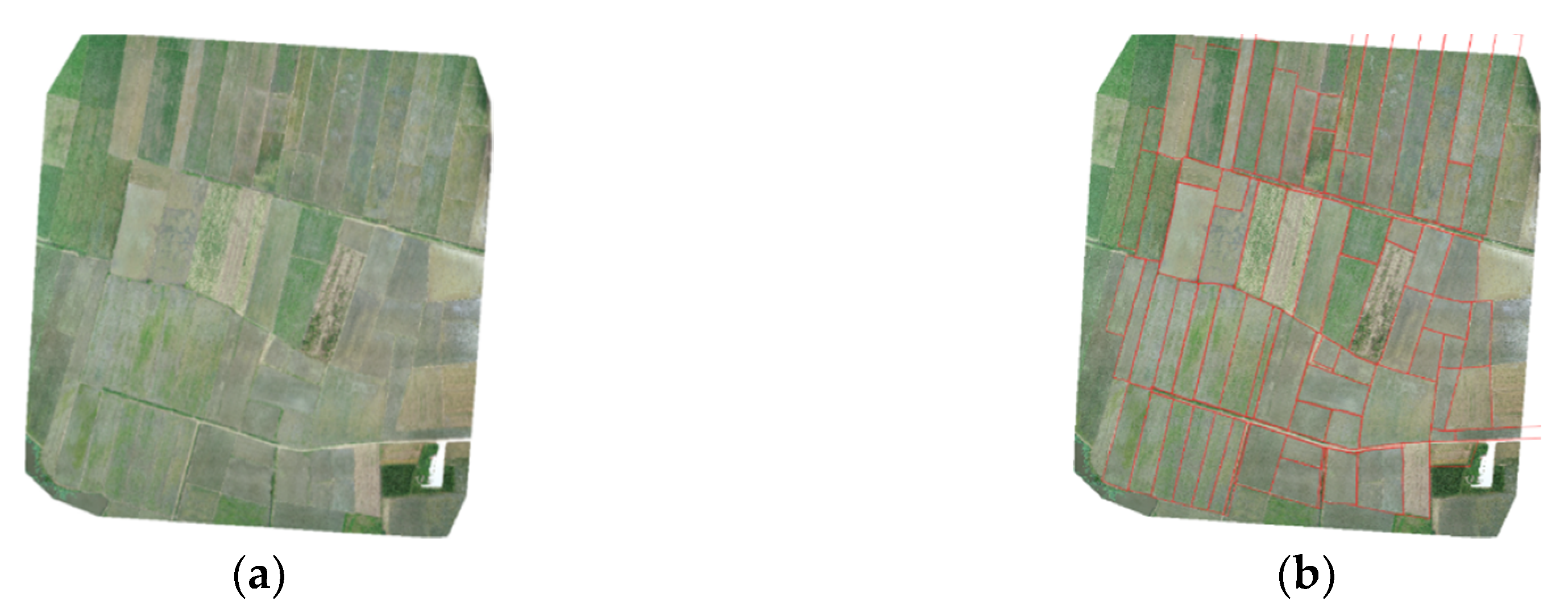
Second, we applied the vector information of the fields to tag the samples with the spatial and temporal information automatically. Therefore, we obtained thousands of samples for the middle-season rice in different periods and places. This automatic tagged method can extend the building method for the remote sensing image dataset.
Last, we use a fine classification method to learn the spatial-temporal information of the middle-season rice. The image dataset can support different deep learning networks and achieve a good result. This strategy of conversion for fine classification of the image dataset will extend the applications for the original deep learning algorithms.

2. Materials and Methods

2.1. Study Area

The growing area of middle-season rice includes more than eight provinces in China and has a subtropical warm and humid monsoon climate. The growing area is approximately 16.5 million square kilometers and accounts for 68.1 percent of the total area sown with rice.
In this paper, the selected villages were located in the middle and east of the mid-season rice production area. Figure 1 shows the selected cities and the villages on the map, where five villages of two cities in Hubei are shown. Village 1 and 2 were selected to be in Xiantao city, southern Hubei province, with a geographical location of longitude 113°36′30″–113°36′47″ and latitude 30°12′40″–30°12′55″. Village 3, 4, and 5 were selected in the administrative region of Zhijiang city, Hubei province, whose geographical location is between longitude 111°25′00″–112°03′00″ east and latitude 30°16′00″–30°40′00″ north. These regions can better reflect the middle and lower reaches of the Yangtze River in China.

2.2. Data Collection and Processing

2.2.1. The UAV and Camera System

We applied the model Phantom 4 of the DJI Spirits series with an RGB camera for data acquisition. The UAV platform and the camera were ordinary consumer products of low cost that are suitable for small areas less than 1 km 2   and half an hour of operation.
Table 1 describes the detailed parameters for the UAV platform and the camera. The model of the UAV is the DJI M200 commercial product, and this UAV can fly with a max speed of wind at 12 m/s, and reach a max speed of 82.8 km per hour. The maximum flying time was about 38 min; thus, we needed to exchange the battery three times for one flight task. The size of the drone was 887 × 880 × 378 mm, and the total payload was approximately 6.14 kg. This platform was equipped with an Inertial Measurement Unit (IMU) and Global Positioning System (GPS) to record the position and pose for each shutting, and we also installed a system clock to record the date and time for the images. The camera system was the Zenmuse X4S, which has 1-inch Complementary Metal-Oxide-Semiconductor (CMOS) sensors in RGB colors. This sensor can acquire images with a resolution of 20 million pixels under a field of view (FOV) of 84°. This camera system is equipped with three-axis consoles for stabilization during the flight. The UAV system and camera are all commercial products and were acquired not equipped.

2.2.2. Phenological Stages

Considering a standardized description and expression for the growth process of middle-season rice, we introduce the term phenological stage in this paper. On the one hand, there are specialized definitions of each phenological stage, and the obvious differences in the stages can be manually judged by a field investigator. On the other hand, the high-resolution monitoring and modeling for the crop growth in each phenological stage can achieve a higher precision yield estimation.
There are models for product assessments based on the phenological stages, and we first adapted the Biologische Bundesanstalt, Bundessortenamt, and Chemical Industry (BBCH) scale [32] as the basis for the division of phenological stages, which uses decimal code to describe the growth of crops. Taking the existing definition of the middle-season rice phenological stage into consideration, we refer to seven phenological stage settings in this paper, that is, the transplanting, tillering, booting, heading, milk, dough, and maturity stages.
Table 2 presents the phenological stages descriptions and provides the judgment of the growing outlook for each stage. We used the changes of leaves, blooming, grains, and the colors of the field to help the investigators decide which stage the field is in during the UAV flight for acquiring photos. Table 3 presents the data acquisition dates for village 2 from 2017 to 2019.
The phenological stages are an important index for growth monitoring not only for middle-season rice but also for a larger category of plants. However, is difficult for the investigators to distinguish tiny differences in a small interval from the text description of phenological stages for middle-season rice. In addition, the middle-season rice in Hubei possesses the same phenological stages, but there is a time difference of one day or several days in dates in different places and in different years. Figure 2 demonstrates an example of the seven phenological stages in the images of village 1 in Xiantao. The color of the images is different at each stage.

2.2.3. Schedule for Data Acquisition

We set the flight altitude of the UAV to 70 m in Xiantao City and 110 m in Zhijiang City, considering the terrain of the villages, and the resolution of the original raster image was 18 cm and 29 cm for different altitudes, respectively. In addition, each image included four bands, that is, the RGB channels and the transparent channel.
We scheduled a weekly data acquisition by UAV in each village by considering the sowing time and the conditions of the field. Village 1 in Xiantao City was the first place for data collection, which began in June 2017, for a total of 11 weeks; the same data collection times were used for village 5 in 2019. In contrast, the other villages, village 2, village 3, and village 4 were also scheduled from June to October lasting for 13 weeks. The difference exists for the first two weeks in the last three villages because the data acquisition started earlier for two weeks.
We scheduled the data collection in each village in strict accordance with the growth cycle of middle-season rice and arranged it with the same flight altitude and the same periods of time from 10 a.m. to 2 p.m. We designed a table to record the data acquisition. Table 3 shows an example for village 2 from 2017 to 2019. We recorded the date for the UAV flight and the raw images.
We set a different overlap from 30 to 45% during the flight according to the colors of the field blocks, with a higher overlap for a tiny difference between the boundaries and a lower overlap for a clear distinction. This is the reason for the sizable difference in the number of images for each time. We applied the Pix4dmapper software as the pre-processing tool for raw images. For data processing, we integrated all the photos of the village into one whole image that was saved as a geotiff format file. Figure 3a shows the result of the ortho-image after processing for the village.
In addition, we scheduled the data acquisition tasks to the members of the agriculture investigation team and arranged a vector data production job for the field blocks as well as the determination job of the block of middle-season rice and the phenological stage. The vector data were processed to match with the images. Figure 3b shows the result for the merging of the vector data with the image. In each field block, we noted the type of crops, and for the middle-season rice, the details of the phenological stage. This work was then repeated during each week. We needed to ensure the correct information regarding the vector and the attribution of each block.
As for the location information, we obtained the information by two methods and used cross-validation to determine the information. The first method derived the information from the matched vector data, and the second method obtained the GPS information for each shooting moment during the flight. For convenience, we set the location information of the selected village information to all images acquired there. Considering the administrative district, we set the hierarchical folders from the village and city to province to store all the images; in this manner, the images can hold the location information on a different scale. The location information was saved as the name of each folder in the saved directory.

3. Methodology

With the purpose of supporting the machine learning methods to identify the images for the correct place and time, we set up the image dataset in three steps. The first step was data preparation. We scheduled the data acquisition to accompany the survey business of the agricultural investigation team of the National Bureau of Statistics. In this stage, we collected the high-resolution images, the vector bounding data of the field block, and the correct attributes for each field block; therefore, we labeled the data for the correct place and phenological stages.
The second stage is for sample generation. We applied commercial software for the image processing, and after that, we developed a tool to obtain the piece of the field with the image and the vector data. We used an extraction algorithm to sample the block images to generate a standard image size for the dataset that was suitable for most machine learning methods. Finally, we tested our image dataset with several machine learning networks, and the results show that the dataset can be used to perform regression by all of the methods with high accuracy.
Figure 4 shows the overview flowchart of this paper and the detailed steps in each stage. As we mentioned above, the vector data of blocks and the labeling data of different phenological stages were collected with the help of investigation members.

3.1. Sample Generation

When we scheduled the data acquisition, we first assigned the data collection task to the investigation member who was on duty for all the data collection in one village. The data collection task in each village included the UAV images, which were recorded in .jpeg format with GPS, and date and time information. Applying Pix4DMapper data processing functions, the original images had been produced into the DOM in geotiff format. Based on the DOM, the agricultural investigation team drew the field blocks in the QGIS system, and the final vector data was in a shape file. The input data included the raster data of DOMs and the vector data of shp files of the field blocks. Additionally, the labeling data were stored in the vector data as attributes. We refer to the field block as the statistical unit, in this manner, we used the geometry area of the vector data to assess the image statistical accuracy.
The generated high-resolution UAV images usually had more details. The larger the image size is, the greater the computational power and video memory needed to be input into the convolutional neural network for processing. It was impossible to use the original image for training or testing by deep learning methods. The images also contained other crops in addition to the middle-season rice. Therefore, we cut the original large-size image into field blocks and used the label information to obtain the blocks of middle-season rice.
First, we clipped the labeled polygonal blocks on the raster image according to the vector. The AOI (area of interest) was applied to the raster image according to the label information in the vector and the polygon vertex coordinates. When the image and the vector data were matched, it was easy to cut the block out of the original image. With the help of the Geospatial Data Abstraction Library (GDAL), we developed a tool to cut hundreds of polygonal image blocks from the image that corresponded to geographical entities in the vector data.
Figure 5a shows a good result. While it is ideal for all vector data to match with the image, an offset is always obtained. Figure 5b shows that the vector data acquired an offset to the field block of the image. There are two possible reasons: one is that an error is generated by projection, and the other reason is because the data changed, or a low-quality vector was produced. We needed a calibration for the whole image with the vector data, or we needed a careful adjustment for the vector data after the data acquisition.
For the five villages and seven phenological stages in each village per year, we first obtained more than 12,000 image blocks. We used the image blocks to generate samples because the different blocks always exhibit a different outlook, even when planting occurs at the same time and with the same kind of seeds. The blocks typically have one kind of plant. Figure 6 shows the original image matched with the vector data in village 1 of 2018 and the generated block images for each field block.
With the help of the vector data, we obtained the block images from the raw data. However, it was still very difficult to cut the samples directly due to the irregular shape and the edge containing redundant pixels. We applied a cross-over strategy for further processing to obtain the ideal small sample from the target polygonal image block, as shown in Figure 7a. The quadrant size was 256 pixels, and only when the quadrants of the four directions existed could we obtain the sample quadrant in the middle. For the whole image, we retrieved all valid quadrants, and from only these valid quadrants could the orange quadrant in Figure 7a be selected as the final sample. The size of the sample depended on the need of the machine learning algorithm; in this paper, we employed pixel sizes of 256 × 256 and 128 × 128.
Even for the ideal matched vector and image pairs, we obtained the block image from the original without a rectangle or square shape, as shown in Figure 7b, and we also found that the pixels near the boundary were always mixed with other features, such as the path or other plants. This block image shows that the image contains many blank pixels and grass pixels. To generate uniform and clear samples, we employ the strategy that begins at the left top of the image, following the sequence from left to right and top to bottom, obeying the cross-quadrant ruler to generate the samples in different sizes.
There was always a clear difference in the texture pattern between the middle-season rice blocks and non-middle-season rice blocks. The samples between block images changed considerably. Figure 8a shows the samples for middle-season rice from the same block image in Xianto. Figure 8b shows the non-middle-season rice feature samples from the same source image.
To organize the image quadrants, we took a hierarchical structure, from district to date and so on. In the naming of the sample file, we adopted the following format: xt_1_70m_rgb_20180613_00002_00001_size_256_rotate_0_step_256.png, where XT refers to the abbreviation of the city name, namely, Xiantao city; one is the first village; 70 m refers to the height at which the drone flies; RGB describes the picture as a three-channel color image; 20180613 refers to the date of image acquisition; 00002 means that the sample square is from lot two after cutting by AOI; 00001 refers to the quadrant number one generated for plot number two; Size_256 is the cut size of 256 × 256; rotate_0 refers to the absence of rotation when cutting the quadrant (rotation angle is zero); step_256 refers to the cutting step size set to 256 pixels (the same as the cutting size); .png is the storage format. Compared with the .tif format, .png not only ensures the lossless storage of quadrant images but also removes information, such as geographical coordinates, thus, saving storage space.

3.2. Dataset Description

3.2.1. The Image Dataset

In this paper, we collected the UAV high-resolution images to generate samples in two cities from 2017 to 2019. Table 4 shows the classes and number of samples in each class. There were seven phenological stages in one year for middle-season rice; we set up seven classes for each stage and one class for the others, so there was a total of eight classes for one city per year. We obtained 120 classes in total with more than 500,000 samples in the dataset.

3.2.2. The Splits of the Dataset

We simply split the total image dataset into two parts by randomly selecting 75% of the images as the training dataset and the other 25% for the testing dataset. All classes had two folders: one contained the training images, and the other folder stored the test images. The example of images for training and testing in Xiantao on 10 August 2017 is shown in Figure 9.

3.2.3. Comparison with Typical Remote Sensing Image Datasets

We compared our UAV image dataset with serval public image datasets for deep learning in Table 5. Many RSIDs are from Google Earth imagery with a spatial resolution from 0.3 to 30 m. The existing image datasets can support the land cover classification, scene classification, and object detection applications. Our UAV image dataset is also suitable for those applications, and, with the labeled semantic of middle-season rice, this dataset can support the semantic classification of rice. The class of the existing RSID has several to hundreds of samples per class, and there was no information regarding the acquisition time and the location.
In our UAV image dataset, the different places and different phenological stages corresponded to one class that had 3000 to 6000 samples. The existing RSIDs do not have the ability to classify or detect features of different times and places. We defined massive classes to represent the spatial and temporal information.

4. Tests and Analysis

To verify the effectiveness of the proposed image dataset, we carried out two tests. The first test was the fine classification for spatial and temporal information by deep learning methods. In this test, we examined the classification of mid-season or not in the two cities and five villages and then examined the seven different phenological stages in different places. We selected the PyTorch deep learning framework and four classical neural network algorithms, namely, AlexNet [33], VGG16 [34], ResNet [35], and DenseNet [36] to test and compare with the UCMerced Land Use Dataset [13] and RSSCN7 Dataset [15].
The training hardware adopted in this paper consisted of an NVIDIA GTX-1080 graphics card with 8 GB of video memory and an NVIDIA TITAN V with 12 GB of video memory.
At the beginning of the first test, we selected 1/10 of the images from the training set for the verification set. We also adjusted the learning rate and other hyperparameters to obtain better performance.
During testing, we carried out the tensor normalization (ToTensor) operation on all test set images; thus, the RGB values of the images that ranged from 0 to 255 were normalized to 0 to 1. We applied standardization accordingly (normalize) to speed up the convergence of the algorithm and subsequently applied random shuffle (shuffle) to the training set. Then, we divided the images into small batches in the network. The batch size of the experiment varied according to the algorithm; in this paper, the value employed in the experiment was between 32 and 128. A larger value of the batch size will significantly improve the speed, but the requirement for video memory will also significantly increase.
During the experiment, we recorded the cross-entropy loss between the prediction result of the test set and the real label by the model obtained through each cycle of (epoch) training. We tested each model for 200 epochs and then calculated the average accuracy for our dataset. The test results are shown in Figure 10. We examined the classification of mid-season or not in different villages, and we added them (places) to the network. In this case, we obtained the 40 classes for identifying the villages in two cities for three years. For the examined seven different phenological stages with the different places, we added them (stages) to the end of the network. The total number of classes was 105 where we could identify each stage of the different villages in each year. The accuracy is the right classification ratio.
While there are large counts of samples in the training set, we obtained the accuracy in the validation set and test set. Table 6 shows the results for classification. On AlexNet, the accuracy of the validation set reached 91.00% in the phenological stages test and 98.01% in the middle rice and non-middle rice classification of different villages. The training session took approximately 13 h.
On VGG16 [37], the accuracy of the validation set reached 95.70% in the phenological stages test and 98.38% in the middle rice and non-middle rice classification of different villages, while the accuracy of the test set only reached 65.07% in the phenological stages test and 86.62% in the middle rice and non-middle rice classification of different villages. The training session took approximately 37 h.
On ResNet-50 [38], the accuracy of the validation set reached 97.50% in the phenological stages test and 98.80% in the middle rice and non-middle rice classification of different villages, while the highest accuracy of the test set was only 75.31% in the phenological stages test and 91.64% in the middle rice and non-middle rice classification of different villages. The training session took approximately 43 h.
On DenseNet-121 [39], the accuracy of the validation set reached 97.80% in the phenological stages test and 98.90% in the middle and non-middle rice classification of different villages, while the accuracy of the test set only reached 74.40% in the phenological stages test and 92.40% in the middle and non-middle rice classification of different villages. The training session took approximately 50 h.
The results show that the UAV image dataset of middle-season rice supported the deep learning classification task of middle-season rice, which lays a foundation for the further addition of the regional classification experiments. The fine classification of images for spatial and temporal information can improve the efficiency for the agricultural investigation team. We needed six members for one village to do the manner classification and two days to finish the works of one phenological stage. By applying the deep learning method to our dataset, two members could finish the same work in two days. The high-resolution image dataset was able to improve the accuracy for agricultural investigation.
After training the models with our dataset, we tested if the reference image dataset could achieve the result by fine classification. We applied the UCMerced Land Use Datasets and RSSCN7 image dataset for testing.
As for the UCMerced Land Use Datasets dataset, we found that 100 images contained agriculture and 92 images were related to rice. We relabeled these images to fit the classification. For the RSSCN7 image dataset, there were about 400 images related to agriculture, and we also relabeled 295 images to fit our test. For the UCMerced Land Use Datasets dataset, we tested for 50 epochs, and we tested the RSSCN7 image dataset for 100 epochs. The accuracy was the average of the cross-entropy loss between the prediction and the labeled information. Table 7 shows the result of the fine classification of different villages of different cities. The two public image datasets had few images for agriculture, and scarce images for middle-season rice. Thus, the models had very low accuracy.
To verify that our image dataset could support the public image classification as land use, we performed the second test. We used the published models and the parameters of classification tasks on three image datasets and compared the results. In this test, AlexNet, VGG, ResNet, and DenseNet were applied for land use classification. The result is shown in Table 8.
For land-use classification, the AlexNet on UCMerced Land Use Data Set obtained 93.1% [40] and RSSCN7 obtained 92.32%, while our image dataset obtained 95.95%. VGG16 achieved 93.98% on the UCMerced Land Use Data Set and 94.62% on the RSSCN 7 dataset [41]. Resnet [40] and DenseNet [42] obtained 91.92% and 97.70% on the UCMerced Land Use Dataset and 96.07% and 97.46% on the RSSCN 7 image dataset, respectively. Our image dataset obtained a higher accuracy classification for all networks.

5. Discussion

The purpose of the paper was to build an image dataset for middle-season rice based on high-resolution UAV images for accurate subclassification of the correct place and correct time by machine learning methods.
The data collected in this paper were based on agricultural investigation, and the operation process will generate considerable business data. To avoid specific business impacts, the generation of the dataset only applies the field block vector data, the place, and the time of collection. Due to business needs, data collection can be conducted on the same village for many years to form periodic image comparisons, which also reduces the amount of manual data processing. After completing the vector data production for field blocks in the first year, the same vector data will be used in subsequent years.
In practice, the vector data of the field block in the village changes little except for the adjustment of farmers in some areas. Due to the need to consider the data accuracy and data precision, this paper does not consider the method of automatic segmentation of land. After the calibration of the image, the vector data of the field block in the survey area can well fit the image. In the areas with large differences, the original image data can be checked or confirmed through field investigation and manually modified to ensure the proper amount of sampling area and the image nesting relationship. Finally, the generation of the standard quadrant can be determined.
The ground resolution of the image was a relatively high resolution of 0.2 m. In this paper, the UAV data collection was conducted for three consecutive years in Hubei province. The collected areas are mostly plains, and the area has an elevation between 20 and 50 m. Therefore, this was not sufficient to represent the middle and lower reaches of the Yangtze River with the large difference in elevation. The plants of middle-season rice may have a different outlook in mountains and hilly landforms. New places should be taken into consideration for further data acquisition.
It is difficult to obtain the time-series data in different locations for rice crops. The growing areas are distributed, and professional information about the growing stages is required. Although we scheduled careful data acquisition tasks and the images are of high quality, the machine learning algorithms still classified two different stages of images as one class. The outlook of the middle-season rice of different growing stages in different places always has little difference. In our implementation, we chose places that had an obvious outlook. The texture pattern of middle-season rice in the earlier phenological stage was uniform for rice shoots scattered in the paddy field. Another difference is that our dataset will add the class when places are extended, and the data continue to be acquired for additional years.
In this paper, we adopted consumer products, employing an unmanned aerial vehicle (UAV) system and a camera from DJI, not professional products with high-level camera modules, and positioning navigation equipment. The multi-resolution construction was only based on the highest resolution using a unified method and resampling generation. Pix4D was used in the image processing in this paper, and the accuracy of the results, the processing method, the degree of automation, and the efficiency of its image processing were not considered for optimization. Based on the processing results of widely accepted commercial software, the data processing time was not evaluated. The workload of data processing was heavy. The UAV image data collected at each sampling point required dozens of hours of image processing time on a single workstation.
Finally, four kinds of neural networks, including AlexNet, VGG, ResNet, and DenseNet, were tested for classification based on this image dataset. Our image dataset obtained a reasonable result of identifying the spatial and temporal information for the images by fine classification. AlexNet [33], VGG16 [34], ResNet [35], and DenseNet [36] achieved more than 90% accuracy. In this situation, our image dataset met the design of the target. We used these models to test with the UCMerced Land Use Dataset [13] and RSSCN7 Dataset [15], and all of them obtained an accuracy of less than 10%. The two image datasets contain few images of middle-season rice, and none of them came from the flight site villages. Therefore, using the public image dataset cannot support this application.
To judge our image set in land use or other public classification tasks, we compared the public two image datasets. The results of AlexNet [40], VGG16 [37] ResNet [38], and DenseNet [42] on the UCMerced Land Use Dataset were lower than our image dataset, due to the image resolution and the samples numbers. The same situation was found for the networks on the RSSCN 7 dataset.
This article does not focus on how to further improve the classification and the innovation of new networks. We only confirmed in this paper that the image dataset provided accurately reflected the situation of middle-season rice in the selected region, particularly at the time and under the specific climatic conditions.

6. Conclusions

This paper presents a high-resolution UAV image dataset of middle-season rice suitable for the middle and lower reaches of the Yangtze River. Through the acquisition of UAV images of five villages of two cities by the Yangtze River in Hubei in the past three years with the same cycle and the manual crop interpretation confirmation of an agricultural survey business, the vector data of regional plots were obtained, and the image dataset of the middle rice growth process was constructed. The dataset was divided into 15 categories according to the place and year.
Each category was subdivided into 11 or 13 phases according to the crop phenological stages, and more than 500,000 samples of size 256 × 256 were obtained in total. After the construction of the dataset, we used four common networks to conduct the binary classification of whether the data represented middle-season rice or not and performed the fine classification for the phenological stages and the place. The results show that this dataset achieved good results in many networks, satisfying the common classification application.
The monitoring of growth for rice crops is an interesting and difficult job. The deep learning method provides a possibility for performing this job. Our dataset supports an important foundation for the reorganization of middle-season rice with the timing of the phenological stages and locations. Combined with agricultural investigation information of the average product for a particular location, this allows us to predict the yield of middle-season rice. For each phenological stage, the agricultural investigator can find abnormal growth and send messages to the farmer.
Due to the limitations of the sample locations, the current datasets well fit the Hubei plains. However, for more suitable implementations for the Yangtze River, we should increase other sampling locations of the middle-season rice provinces, in particular the hilly and mountainous areas. Further, we will apply the new UAV system equipped with the multispectral sensors to support complex applications and improve the intelligent and automatic level of the agricultural production process.

Author Contributions

Conceptualization, Dongbo Zhou and Jie Yu; Data curation, Hao Li; Formal analysis, Hao Li and Jie Yu; Funding acquisition, Dongbo Zhou, Hao Li, and Jie Yu; Investigation, Jie Yu; Methodology, Dongbo Zhou and Shuangjian Liu; Project administration, Dongbo Zhou; Resources, Hao Li; Software, Dongbo Zhou and Shuangjian Liu; Validation, Dongbo Zhou, Shuangjian Liu, and Jie Yu; Visualization, Shuangjian Liu and Hao Li; Writing—original draft, Dongbo Zhou; Writing—review and editing, Jie Yu. All authors have read and agreed to the published version of the manuscript.

Funding

This research was funded by the National Natural Science Foundation of China, grant numbers 41671377, 41501463, and 61807013, and the National Key Technologies Research and Development Program of China under Grant 2016YFB0502604.

Conflicts of Interest

The authors declare no conflict of interest.

References

  1. Seck, P.A.; Diagne, A.; Mohanty, S.; Wopereis, M.C.S. Crops that feed the world 7: Rice. Food Secur. 2012, 4, 7–24. [Google Scholar] [CrossRef]
  2. Wang, P.; Zhang, Z.; Song, X.; Chen, Y.; Wei, X.; Shi, P.; Tao, F. Temperature variations and rice yields in China: Historical contributions and future trends. Clim. Chang. 2014, 124, 777–789. [Google Scholar] [CrossRef]
  3. Peralta, N.R.; Assefa, Y.; Du, J.; Barden, C.J.; Ciampitti, I.A. Mid-Season high-resolution satellite imagery for forecasting site-specific corn yield. Remote Sens. 2016, 8, 848. [Google Scholar] [CrossRef] [Green Version]
  4. Weiss, M.; Jacob, F.; Duveiller, G. Remote sensing for agricultural applications: A meta-review. Remote Sens. Environ. 2020, 236, 111402. [Google Scholar] [CrossRef]
  5. Karthikeyan, L.; Chawla, I.; Mishra, A.K. A review of remote sensing applications in agriculture for food security: Crop growth and yield, irrigation, and crop losses. J. Hydrol. 2020, 586, 124905. [Google Scholar] [CrossRef]
  6. Bah, M.; Hafiane, A.; Canals, R. Deep learning with unsupervised data labeling for weed detection in line crops in UAV images. Remote Sens. 2018, 10, 1690. [Google Scholar] [CrossRef] [Green Version]
  7. Yao, H.; Qin, R.; Chen, X. Unmanned aerial vehicle for remote sensing applications—A review. Remote Sens. 2019, 11, 1–22. [Google Scholar] [CrossRef]
  8. Yang, Q.; Shi, L.; Han, J.; Yu, J.; Huang, K. A near real-time deep learning approach for detecting rice phenology based on UAV images. Agric. For. Meteorol. 2020, 287, 107938. [Google Scholar] [CrossRef]
  9. Lecun, Y.; Bengio, Y.; Hinton, G. Deep learning. Nature 2015, 521, 436–444. [Google Scholar] [CrossRef]
  10. Wu, J.; Yang, G.; Yang, X.; Xu, B.; Han, L.; Zhu, Y. Automatic counting of in situ rice seedlings from UAV images based on a deep fully convolutional neural network. Remote Sens. 2019, 11, 691. [Google Scholar] [CrossRef] [Green Version]
  11. Zhou, W.; Newsam, S.; Li, C.; Shao, Z. PatternNet: A benchmark dataset for performance evaluation of remote sensing image retrieval. ISPRS J. Photogramm. Remote Sens. 2018, 145, 197–209. [Google Scholar] [CrossRef] [Green Version]
  12. Han, W.; Feng, R.; Wang, L.; Cheng, Y. A semi-supervised generative framework with deep learning features for high-resolution remote sensing image scene classification. ISPRS J. Photogramm. Remote Sens. 2018, 145, 23–43. [Google Scholar] [CrossRef]
  13. Yang, Y.; Newsam, S. Geographic image retrieval using invariant features. IEEE Trans. Geosci. Remote Sens. 2013, 51, 818–832. [Google Scholar] [CrossRef]
  14. Sheng, G.; Yang, W.; Xu, T.; Sun, H. High-Resolution satellite scene classification using a sparse coding based multiple feature combination. Int. J. Remote Sens. 2012, 33, 2395–2412. [Google Scholar] [CrossRef]
  15. Zou, Q.; Ni, L.; Zhang, T.; Wang, Q. Deep learning based feature selection for remote sensing scene classification. IEEE Geosci. Remote Sens. Lett. 2015, 12, 2321–2325. [Google Scholar] [CrossRef]
  16. Long, Y.; Gong, Y.; Xiao, Z.; Liu, Q. Accurate object localization in remote sensing images based on convolutional neural networks. IEEE Trans. Geosci. Remote Sens. 2017, 55, 2486–2498. [Google Scholar] [CrossRef]
  17. Cheng, G.; Han, J.; Lu, X. Remote sensing image scene classification: Benchmark and state of the art. Proc. IEEE 2017, 105, 1865–1883. [Google Scholar] [CrossRef] [Green Version]
  18. Xia, G.S.; Hu, J.; Hu, F.; Shi, B.; Bai, X.; Zhong, Y.; Zhang, L.; Lu, X. AID: A benchmark data set for performance evaluation of aerial scene classification. IEEE Trans. Geosci. Remote Sens. 2017, 55, 3965–3981. [Google Scholar] [CrossRef] [Green Version]
  19. Xiao, Z.; Liu, Q.; Tang, G.; Zhai, X. Elliptic Fourier transformation-based histograms of oriented gradients for rotationally invariant object detection in remote-sensing images. Int. J. Remote Sens. 2015, 36, 618–644. [Google Scholar] [CrossRef]
  20. Zhang, Y.; Yuan, Y.; Feng, Y.; Lu, X. Hierarchical and robust convolutional neural network for very high-resolution remote sensing object detection. IEEE Trans. Geosci. Remote Sens. 2019, 57, 5535–5548. [Google Scholar] [CrossRef]
  21. Maggiori, E.; Tarabalka, Y.; Charpiat, G.; Alliez, P. Can semantic labeling methods generalize to any city? the inria aerial image labeling benchmark. In Proceedings of the IEEE International Geoscience and Remote Sensing Symposium (IGARSS), Fort Worth, TX, USA, 23–28 July 2017; Volume 2017, pp. 3226–3229. [Google Scholar] [CrossRef] [Green Version]
  22. Basu, S.; Ganguly, S.; Mukhopadhyay, S.; DiBiano, R.; Karki, M.; Nemani, R. DeepSat—A learning framework for satellite imagery. In Proceedings of the 23rd SIGSPATIAL International Conference on Advances in Geographic Information Systems, Washington, DC, USA, 3–6 November 2015; pp. 1–22. [Google Scholar] [CrossRef]
  23. Kuznetsova, A.; Rom, H.; Alldrin, N.; Uijlings, J.; Krasin, I.; Pont-Tuset, J.; Kamali, S.; Popov, S.; Malloci, M.; Kolesnikov, A.; et al. The Open Images Dataset V4: Unified image classification, object detection, and visual relationship detection at scale. Int. J. Comput. Vis. 2020, 128, 1956–1981. [Google Scholar] [CrossRef] [Green Version]
  24. Delmerico, J.; Cieslewski, T.; Rebecq, H.; Faessler, M.; Scaramuzza, D. Are we ready for autonomous drone racing? The UZH-FPV drone racing dataset. In Proceedings of the 2019 International Conference on Robotics and Automation, Montreal, QC, Canada, 20–24 May 2019; pp. 6713–6719. [Google Scholar] [CrossRef]
  25. Lyu, Y.; Vosselman, G.; Xia, G.S.; Yilmaz, A.; Yang, M.Y. UAVid: A semantic segmentation dataset for UAV imagery. ISPRS J. Photogramm. Remote Sens. 2020, 165, 108–119. [Google Scholar] [CrossRef]
  26. Zhu, P.; Wen, L.; Du, D.; Bian, X.; Hu, Q.; Ling, H. Vision meets drones: Past, present and future. arXiv 2020, arXiv:1804.07437, 1–20. [Google Scholar]
  27. Chen, Y.Y.; Wang, Y.; Lu, P.; Chen, Y.Y.; Wang, G. Large-scale structure from motion with semantic constraints of aerial images. In Proceedings of the Chinese Conference on Pattern Recognition and Computer Vision (PRCV), Guangzhou, China, 23–26 November 2018; pp. 347–359. [Google Scholar] [CrossRef]
  28. Christian, M.; Michael, M.; Nilolaus, H.; Jesus Pestana, P.; Friendrich, F. Semantic Drone Dataset. Available online: http://www.dronedataset.icg.tugraz.at/ (accessed on 2 October 2020).
  29. Li, S.; Yeung, D.-Y. Visual object tracking for unmanned aerial vehicles: A benchmark and new motion models. In Proceedings of the Thirty-First AAAI Conference on Artificial Intelligence, San Francisco, CA, USA, 4–9 February 2017; pp. 4140–4146. [Google Scholar] [CrossRef]
  30. Mueller, M.; Smith, N.; Ghanem, B. A Benchmark and Simulator for UAV Tracking. In Lecture Notes in Computer Science; Springer: Berlin, Germany, 2016. [Google Scholar] [CrossRef]
  31. Duarte-Carvajalino, J.; Alzate, D.; Ramirez, A.; Santa-Sepulveda, J.; Fajardo-Rojas, A.; Soto-Suárez, M. Evaluating late blight severity in potato crops using unmanned aerial vehicles and machine learning algorithms. Remote Sens. 2018, 10, 1513. [Google Scholar] [CrossRef] [Green Version]
  32. Lancashier, P.D.; Bleiholder, H.; Van Den Boom, T.; Langeluddeke, P.; Stauss, R.; Weber, E.; Witzenberger, A. A uniform decimal code for growth stages of crops and weeds. Ann. Appl. Biol. 1991, 119, 561–601. [Google Scholar] [CrossRef]
  33. Krizhevsky, A.; Sutskever, I.; Hinton, G.E. ImageNet classification with deep convolutional neural networks. Adv. Neural Inf. Process. Syst. 2012, 25. [Google Scholar] [CrossRef]
  34. Simonyan, K.; Zisserman, A. Very deep convolutional networks for large-scale image recognition. In Proceedings of the International Conference on Learning Representations, San Diego, CA, USA, 7–9 May 2015; pp. 1–14. [Google Scholar]
  35. He, K.; Zhang, X.; Ren, S.; Sun, J. Deep residual learning for image recognition. In Proceedings of the IEEE Conference on Computer Vision and Pattern Recognition (CVPR), Las Vegas, NV, USA, 27–30 June 2016; Volume 2016, pp. 770–778. [Google Scholar] [CrossRef] [Green Version]
  36. Huang, G.; Liu, Z.; Van Der Maaten, L.; Weinberger, K.Q. Densely connected convolutional networks. In Proceedings of the 30th IEEE Conference on Computer Vision and Pattern Recognition, CVPR 2017, Honolulu, HI, USA, 21–26 July 2017; pp. 2261–2269. [Google Scholar] [CrossRef] [Green Version]
  37. Mahdianpari, M.; Salehi, B.; Rezaee, M.; Mohammadimanesh, F.; Zhang, Y. Very deep convolutional neural networks for complex land cover mapping using multispectral remote sensing imagery. Remote Sens. 2018, 10, 1119. [Google Scholar] [CrossRef] [Green Version]
  38. Zhang, W.; Tang, P.; Zhao, L. Remote sensing image scene classification using CNN-CapsNet. Remote Sens. 2019, 11. [Google Scholar] [CrossRef] [Green Version]
  39. Cui, W.; Wang, F.; He, X.; Zhang, D.; Xu, X.; Yao, M.; Wang, Z.; Huang, J. Multi-Scale semantic segmentation and spatial relationship recognition of remote sensing images based on an attention model. Remote Sens. 2019, 11, 1044. [Google Scholar] [CrossRef] [Green Version]
  40. Piramanayagam, S.; Saber, E.; Schwartzkopf, W.; Koehler, F. Supervised classification of multisensor remotely sensed images using a deep learning framework. Remote Sens. 2018, 10, 1429. [Google Scholar] [CrossRef] [Green Version]
  41. Hoffmann, E.J.; Wang, Y.; Werner, M.; Kang, J.; Zhu, X.X. Model fusion for building type classification from aerial and street view images. Remote Sens. 2019, 11, 1259. [Google Scholar] [CrossRef] [Green Version]
  42. Zhang, Y.; Gong, W.; Sun, J.; Li, W. Web-Net: A novel nest networks with ultra-hierarchical sampling for building extraction from aerial imageries. Remote Sens. 2019, 11, 1897. [Google Scholar] [CrossRef] [Green Version]
Figure 1. The selected Hubei province for middle-season rice in China. (a) The two selected cities in Hubei; the left city is Zhijiang and the right city is Xiantao; (b) the selected villages 3 and 4 in Zhijiang city, where we set three flight sites for UAV data acquisition in village 3 and two flight sites for data acquisition in village 4. We acquired the data for field blocks, not for the whole village.
Ijgi 09 00728 g001
Figure 2. The seven phenological stages for village 1 in Xiantao. (a) The transplanting stage acquired on 13 June 2018; (b) the tillering stage acquired on 13 July 2018; (c) the booting stage acquired on 19 July 2018; (d) the heading stage acquired on 3 August 2018; (e) the milk stage acquired on 16 August 2018; (f) the dough stage acquired on 30 August 2018; (g) the maturity stage acquired on 11 September 2018.
Ijgi 09 00728 g002
Figure 3. The photos acquired by UAV and the result as the ortho images. (a) The ortho image for one village processed after Pix4D; (b) the image merged with vector data for field blocks.
Ijgi 09 00728 g003
Figure 4. The overview flowchart of the processing. This is divided into three steps. The data preparation is for the data acquisition and preparation. The generation stage is building the dataset, and the test stage is the evaluation of the dataset.
Ijgi 09 00728 g004
Figure 5. A field block cut from the original image with the help of vector data. (a) The matched block cut from the image with the help of the vector; (b) the field block that acquires an offset to the image because of the shape change that occurred in different years.
Ijgi 09 00728 g005
Figure 6. The original image matched with the vector data and then generated as block images for each field block. (a) The original image of the village matched with the vector data; (b) parts of the block images for each field block.
Ijgi 09 00728 g006
Figure 7. The sample using a cross-over strategy. (a) The cross-quadrant for sampling selection; (b) the processing for the field block.
Ijgi 09 00728 g007
Figure 8. The results for the samples were generated from one field block. (a) The samples from middle-season rice in village 1 of Xiantao; (b) the samples from a non-middle-season rice field block in the same place.
Ijgi 09 00728 g008
Figure 9. The samples for the training dataset and testing dataset from Xiantao in 2017: (a) 75% of images were acquired on 14 June for the training dataset; (b) 25% of images were acquired on 10 August for testing.
Ijgi 09 00728 g009
Figure 10. The test results of the accuracy for the binary classification and eight classification experiments. (a) The accuracy of rice and non-rice classification and (b) the accuracy of eight classifications of the different phenological stages.
Ijgi 09 00728 g010
Table 1. The detailed information of the unmanned aerial vehicle (UAV) and camera system.
UAV and CameraType and SeriesParameters
UAVDJI M200Flying time: 38 min
Max speed: 82.8 km/h
Weight: 6.14 kg
Max flying height: 120 m
CameraZenmuse X4S1-inch CMOS
20 million pixels
8.8 mm/F2.8-11 FOV 84°
Spatial resolution: 0.2 m
ISO: 100–12800
Table 2. The seven phenological stages for middle-season rice.
IndexPhenologicalStage DescriptionGrowing Outlook
1TransplantingSeeding and first few leaves have unfoldedA leaf is born every three to four days and the seed roots are replaced by secondary roots
2TilleringMore than nine tillers are visibleThe individual rice leaf splits
3BootingMore nodes are detectable, and the flag leaf sheathe is swollenThe time from the exposure of the leaf pillow of the sword leaf to the first rice tip is approximately nine days
4Heading50% of plants are in bloomHalf of the rice ears come out of the sheaths
5MilkFirst grains are visible and milky ripeMore than 50% of the grain contents are filled with shell in the state of whey
6DoughGrain contents beginning to be concentratedMore than 50% of the grain contents are concentrated without any whey
7MaturityGrains become yellow and the leaves are discolored or fallenApproximately 90% of the grains are yellow and the grains become solid
Table 3. The record of data acquisition on different dates for village 2 from 2017 to 2019.
Phenological StagesDateNumber of ImagesDateNumber of ImagesDateNumber of Images
Transplanting6 June 2017908713 June 201891975 June 20198859
13 June 2017865221 June 2018851811 June 20198412
20 June 2017756926 June 2018618619 June 20196203
27 June 2017733213 July 2018745327 June 20197510
Tillering5 July 2017709919 July 201871834 July 20197211
12 July 2017811226 July 2018828112 July 20198302
Booting19 July 201771933 August 2018728218 July 20197195
26 July 2017776811 August 2018786625 July 20197764
Heading2 August 2017790116 August 201878242 August 20197904
9 August 2017801223 August 201881028 August 20198206
Milk16 August 2017655230 August 2018647217 August 20196632
Dough23 August 201769116 September 2018687325 August 20196993
Maturity30 August 2017688511 September 201868222 September 20196932
Table 4. The dataset from 2017 to 2019 in Hubei province, illustrated by two cities and five villages, with seven phenological stages.
ProvinceCityVillageYearClassesSamples
HubeiXiantao Village 12017849,348
2018848,670
2019848,843
Village 22017822,617
2018822,242
2019822,315
Zhijiang Village 32017854,425
2018853,801
2019853,967
Village 42017840,374
2018839,758
2019839,819
Village 52017825,612
2018825,501
2018825,930
Table 5. The comparison of the typical Remote Sensing Image Dataset (RSID).
RSIDSourceClasses/TimeImagesResolutionApplication
UCLUGoogle211000.3 mClassification
RSSCN7Google72800N/AClassification
NWPU-RESISC45Google4531,5000.2–30 mClassification
RSOD-DatasetGoogle and Tianditu423260.3–2 mObject Detection
DOTA-v1.5Google and GF-11528060.3–2 mObject Detection
UAVidUAV Images8300N/ASemantic Classification
visDrone2020UAV Images1010,209N/AObject Detection
Our DatasetUAV Images120>500,0000.2 mSemantic and Scene Classification
Table 6. The accuracy of fine classification by using four networks.
NetworksValidation Set Test SetTraining Hours
AlexNet (stages)91.00%58.9%13 h
AlexNet (places)98.01%86.57%
VGG16 (stages)95.70%65.07%37 h
VGG16 (places)98.38%86.62%
ResNet-50 (stages)97.50%65.07%43 h
ResNet-50 (places)98.38%86.62%
DenseNet-121 (stages)97.80%74.40%50 h
DenseNet-121 (places)98.90%92.40%
Table 7. The accuracy of fine classification with two public image datasets.
NetworksUCMerced Land Use DatasetsRSSCN7 Dataset
AlexNet (places)3.5%3.3%
VGG16 (places)5.22%5.05%
ResNet-50 (places)7.42%7.18%
DenseNet-121 (places)9.46%9.22%
Table 8. Comparing with two datasets using four classic networks.
NetworksOur Dataset UCMerced_Land Use DatasetRSSCN7 Dataset
AlexNet 95.95%93.1%92.32%
VGG 97.62%93.98%94.62%
ResNet 96.43%91.90%96.07%
DenseNet98.62%97.70%97.46%
Publisher’s Note: MDPI stays neutral with regard to jurisdictional claims in published maps and institutional affiliations.

