An Efficient Row Key Encoding Method with ASCII Code for Storing Geospatial Big Data in HBase

 , , ,
, , ,  , ,
, ,  and
and 
Abstract
1. Introduction
2. Methodology
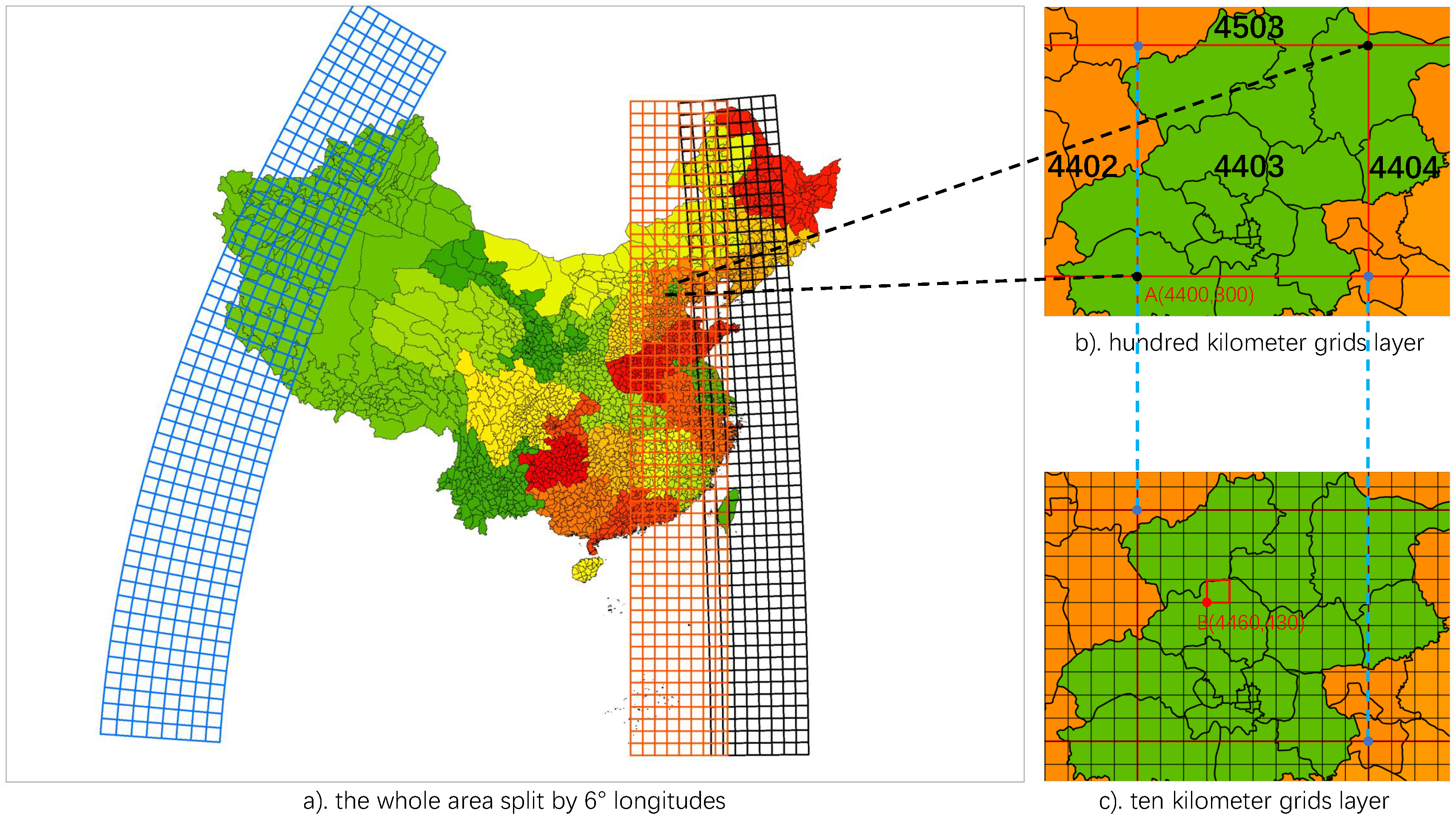
2.1. Spatial Index Multi-Grid
2.1.1. Spatial Reference
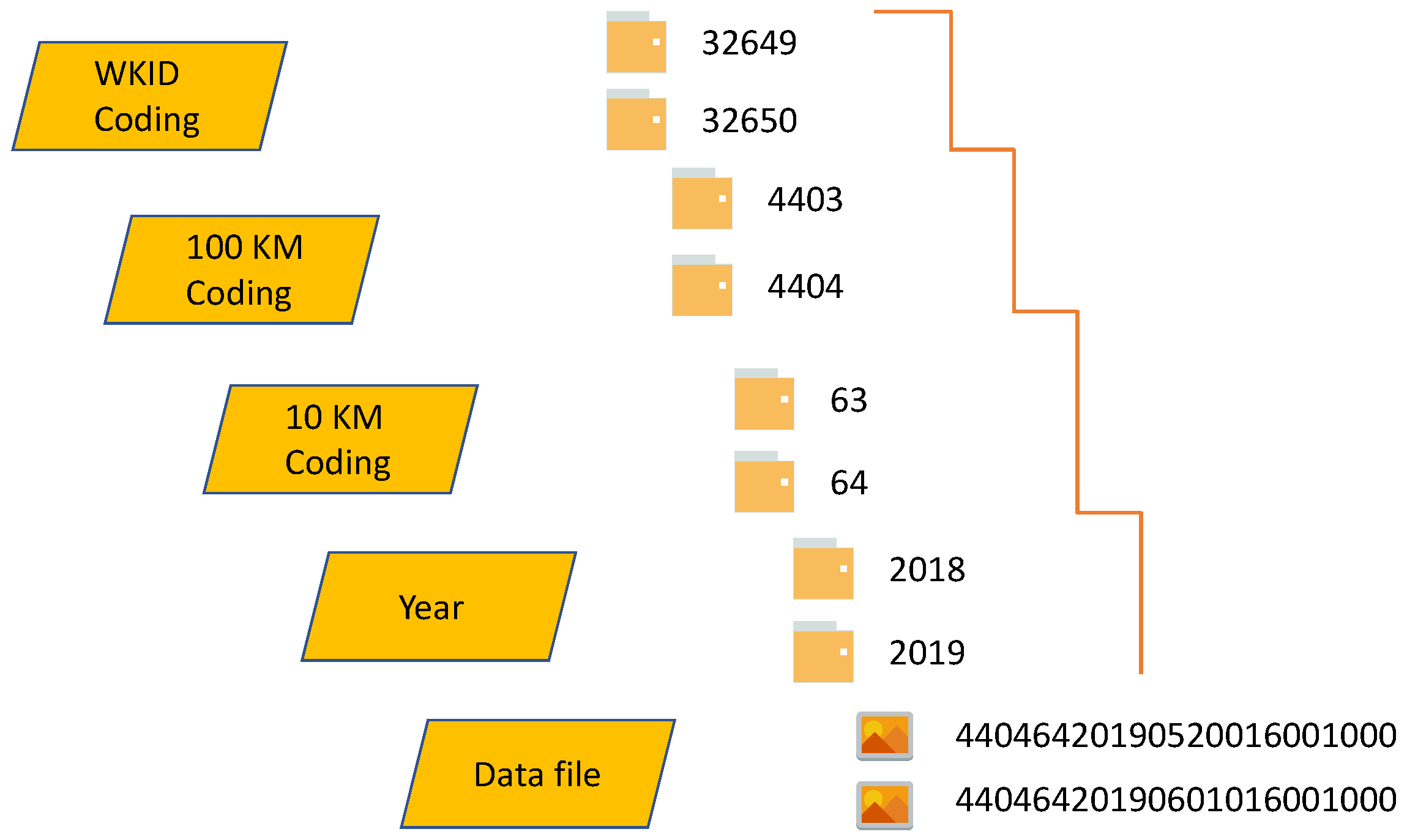
2.1.2. Partition and Coding
2.2. Spatio-Temporal HBase Table Based on RDCRMG
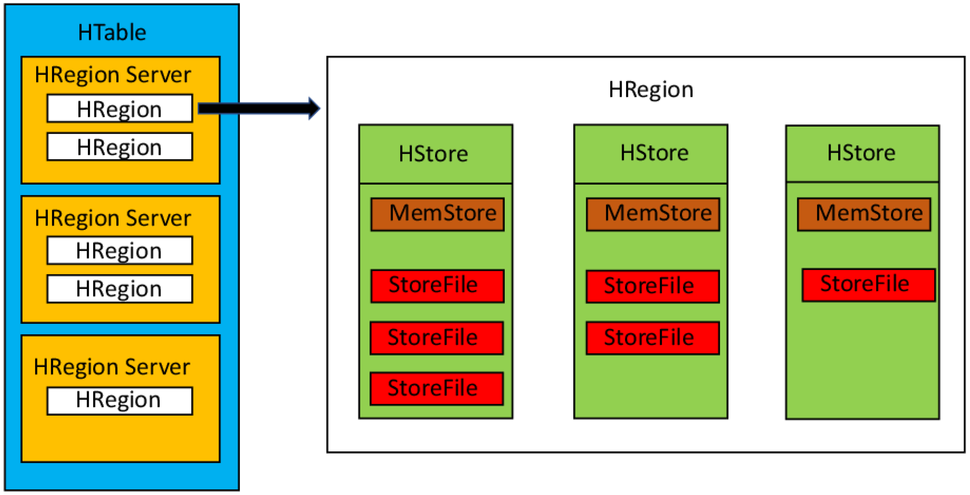
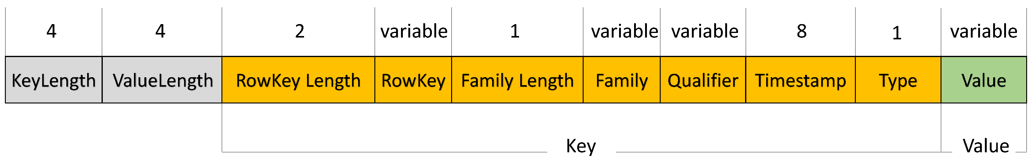
2.2.1. The Structure of a HBase Table
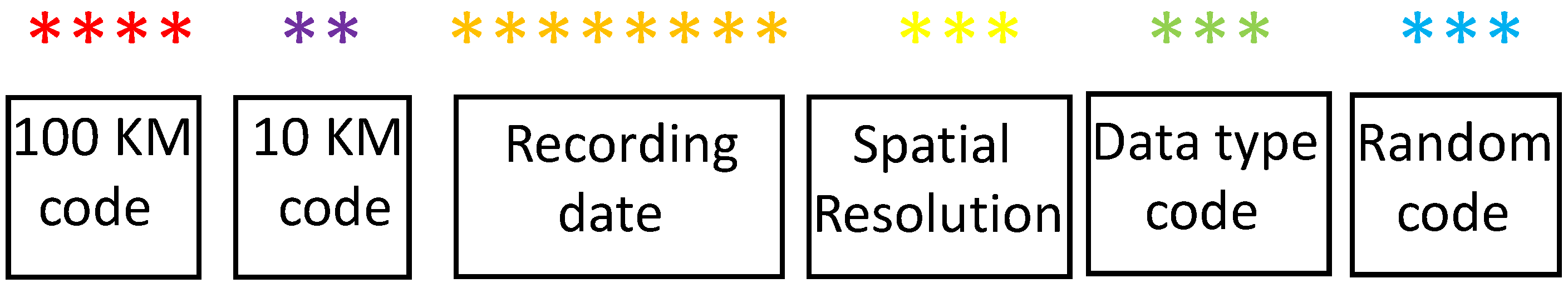
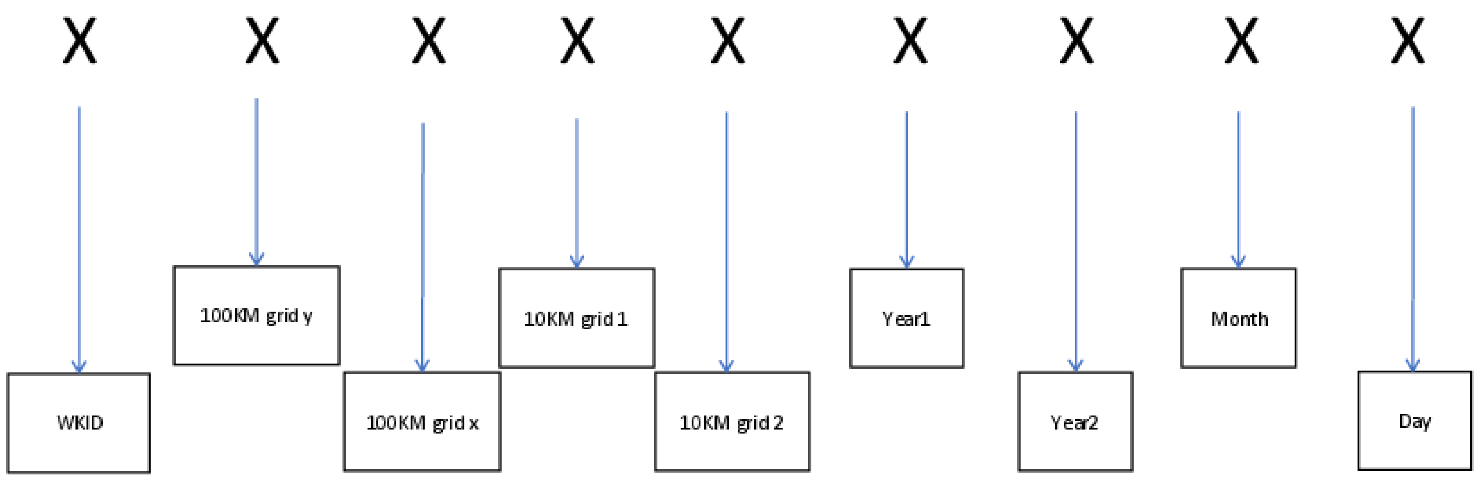
2.2.2. The Design of the Row Key
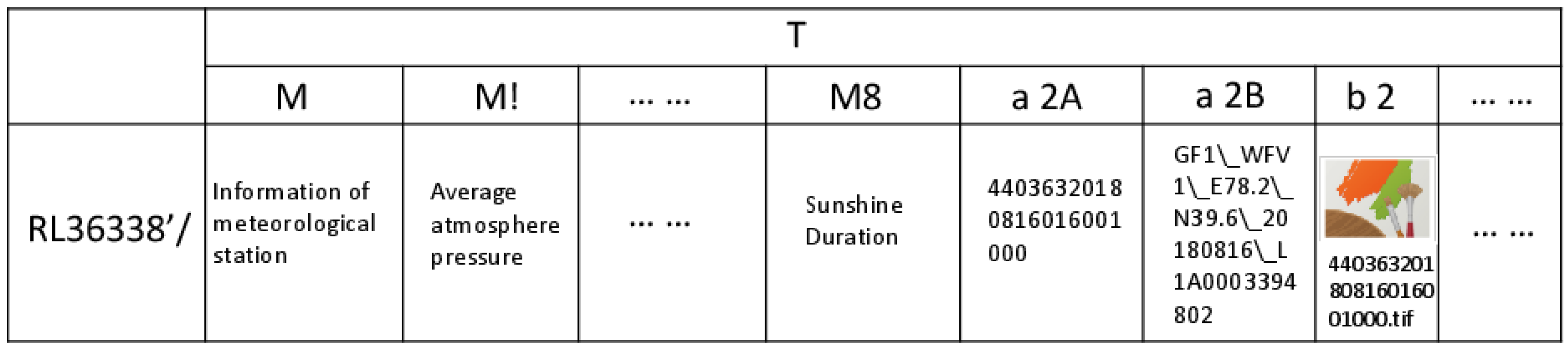
2.2.3. The Design of the Column Family
2.3. Improved Spatio-Temporal Model
2.3.1. Row Key Based on ASCII Code
2.3.2. Columns Based on ASCII Code
3. Results
3.1. Experiment Design
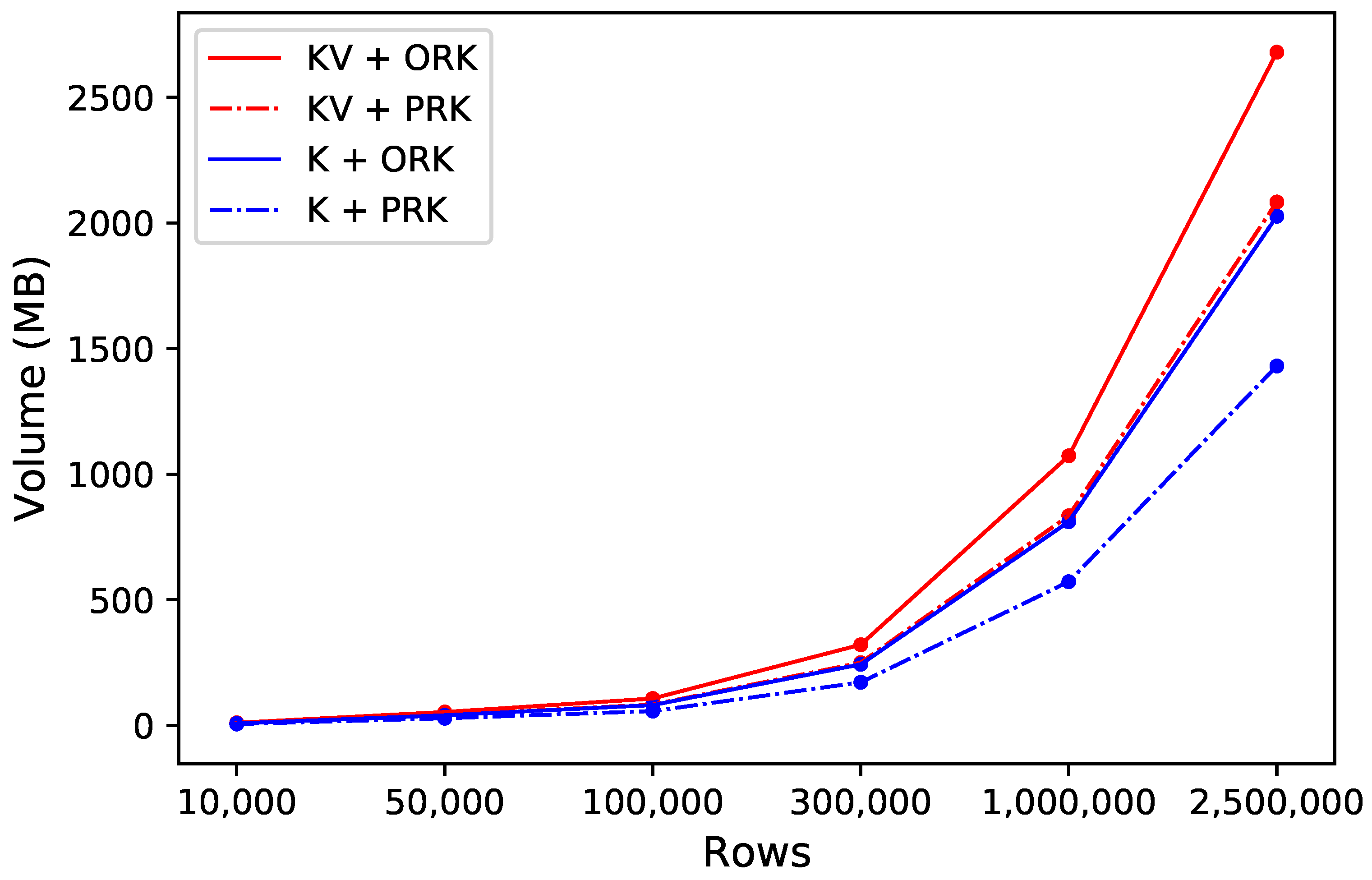
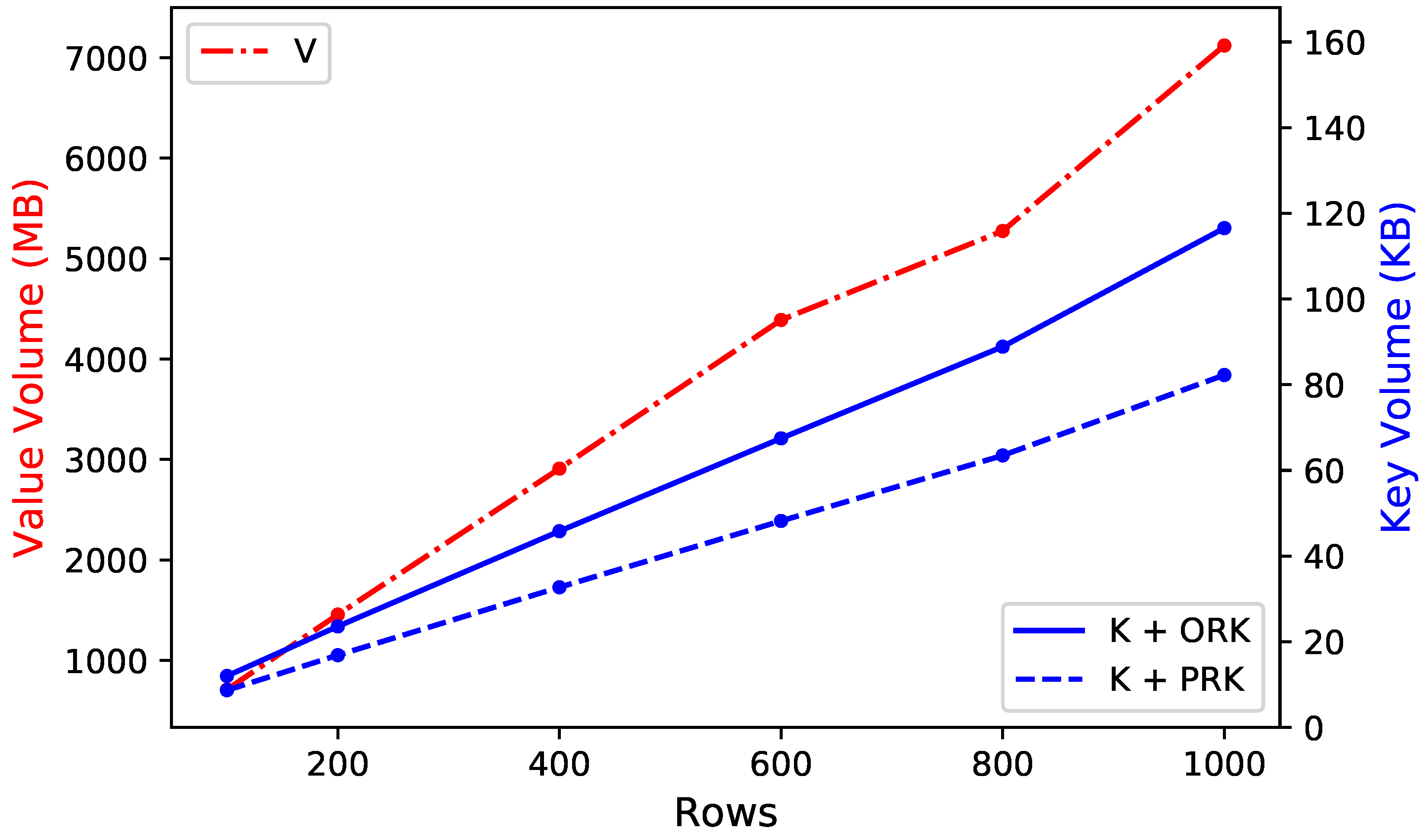
3.2. Row Key Compression Efficiency
3.3. Data Query Efficiency
3.3.1. Random Query
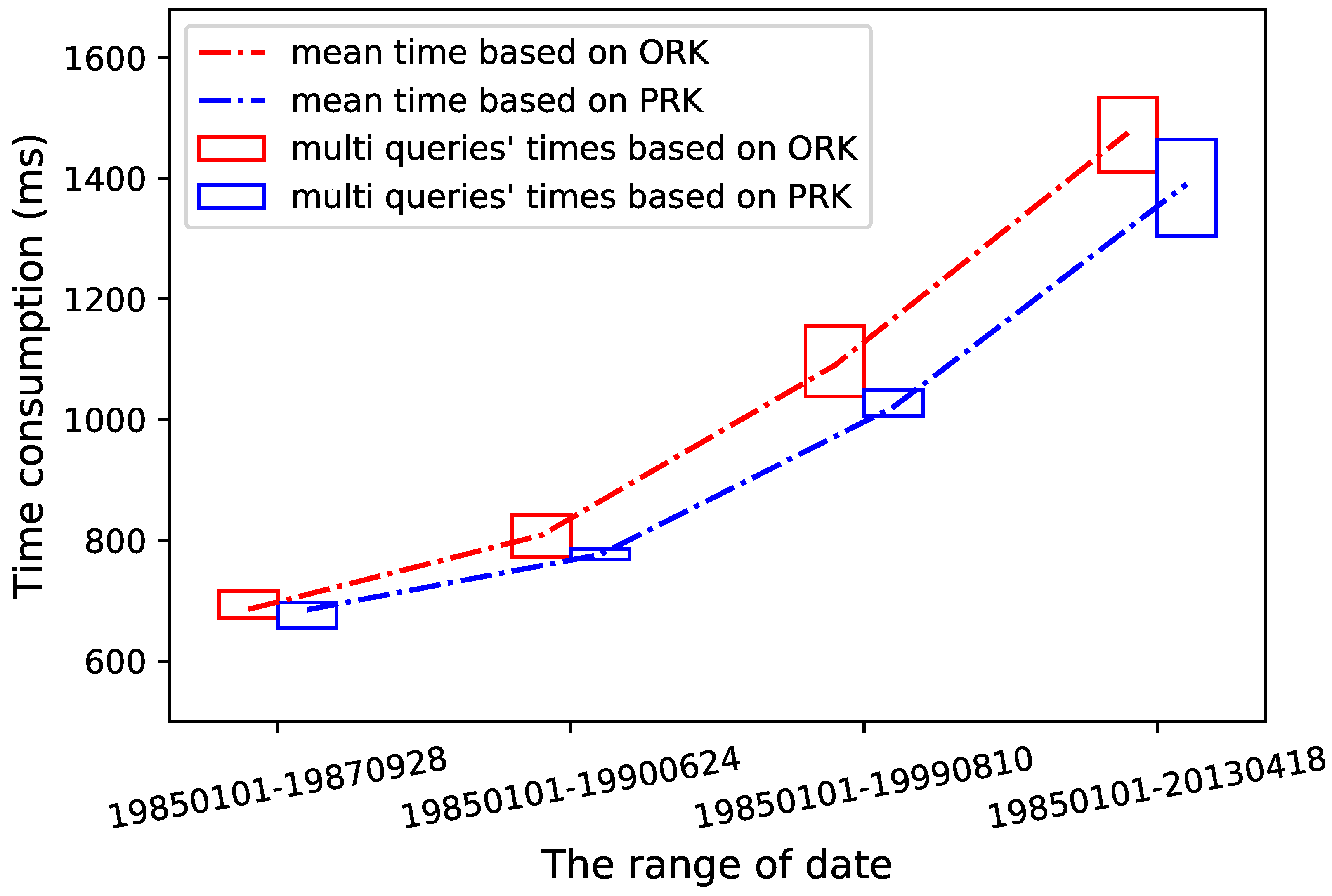
3.3.2. Region Query
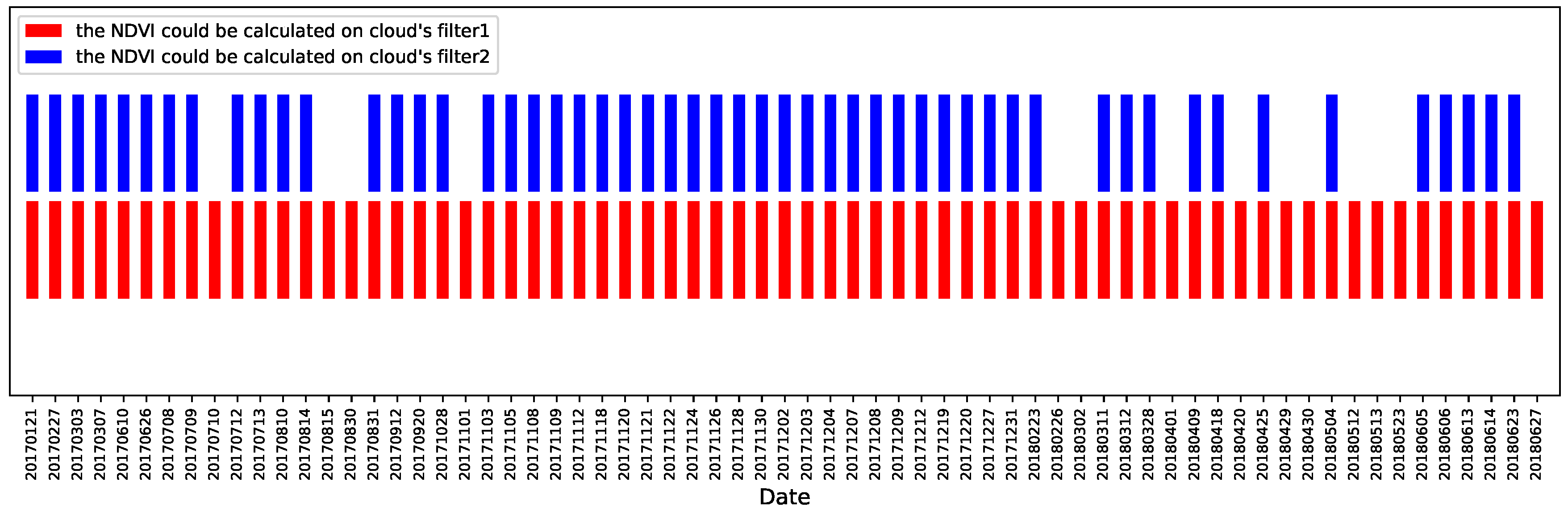
3.4. Application to Spatio-Temporal Calculation
4. Discussion
5. Conclusions
Author Contributions
Funding
Acknowledgments
Conflicts of Interest
Abbreviations
| ASCII | American Standard Code for Information Interchange |
| GF-1 | GaoFen No.1 |
| NDVI | Normalized Difference Vegetation Index |
| UTM | Universal Transverse Mercator |
| HDFS | Hadoop Distributed File System |
| RDCRMG | Raster Dataset Clean and Reconstitution Multi-Grid |
| WGS 84 | World Geodetic System 1984 |
| WKID | Spatial Reference System’s Well-Known ID |
References
- Nativi, S.; Mazzetti, P.; Santoro, M.; Papeschi, F.; Craglia, M.; Ochiai, O. Big data challenges in building the global earth observation system of systems. Environ. Model. Softw. 2015, 68, 1–26. [Google Scholar] [CrossRef]
- Zhu, X.; Cai, F.; Tian, J.; Williams, T. Spatiotemporal fusion of multisource remote sensing data: Literature survey, taxonomy, principles, applications, and future directions. Remote Sens. 2018, 10, 527. [Google Scholar]
- Wei, X.; Duan, Y.; Liu, Y.; Jin, S.; Sun, C. Onshore-offshore wind energy resource evaluation based on synergetic use of multiple satellite data and meteorological stations in Jiangsu Province, China. Front. Earth Sci. 2019, 13, 132–150. [Google Scholar] [CrossRef]
- Yao, X.; Li, G. Big spatial vector data management: A review. Big Earth Data 2018, 2, 108–129. [Google Scholar] [CrossRef]
- He, W.; Yokoya, N. Multi-Temporal Sentinel-1 and-2 Data Fusion for Optical Image Simulation. ISPRS Int. J. Geo-Inf. 2018, 7, 389. [Google Scholar] [CrossRef]
- Tan, Z.; Yue, P.; Di, L.; Tang, J. Deriving high spatiotemporal remote sensing images using deep convolutional network. Remote Sens. 2018, 10, 1066. [Google Scholar] [CrossRef]
- Ghamisi, P.; Rasti, B.; Yokoya, N.; Wang, Q.; Hofle, B.; Bruzzone, L.; Bovolo, F.; Chi, M.; Anders, K.; Gloaguen, R.; et al. Multisource and multitemporal data fusion in remote sensing: A comprehensive review of the state of the art. IEEE Geosci. Remote Sens. Mag. 2019, 7, 6–39. [Google Scholar] [CrossRef]
- Zhuo, W.; Huang, J.; Li, L.; Zhang, X.; Ma, H.; Gao, X.; Huang, H.; Xu, B.; Xiao, X. Assimilating soil moisture retrieved from Sentinel-1 and Sentinel-2 data into WOFOST model to improve winter wheat yield estimation. Remote Sens. 2019, 11, 1618. [Google Scholar] [CrossRef]
- Huang, J.; Sedano, F.; Huang, Y.; Ma, H.; Li, X.; Liang, S.; Tian, L.; Zhang, X.; Fan, J.; Wu, W. Assimilating a synthetic Kalman filter leaf area index series into the WOFOST model to improve regional winter wheat yield estimation. Agric. For. Meteorol. 2016, 216, 188–202. [Google Scholar] [CrossRef]
- Huang, J.; Tian, L.; Liang, S.; Ma, H.; Becker-Reshef, I.; Huang, Y.; Su, W.; Zhang, X.; Zhu, D.; Wu, W. Improving winter wheat yield estimation by assimilation of the leaf area index from Landsat TM and MODIS data into the WOFOST model. Agric. For. Meteorol. 2015, 204, 106–121. [Google Scholar] [CrossRef]
- Lewis, A.; Oliver, S.; Lymburner, L.; Evans, B.; Wyborn, L.; Mueller, N.; Raevksi, G.; Hooke, J.; Woodcock, R.; Sixsmith, J.; et al. The Australian geoscience data cube—foundations and lessons learned. Remote Sens. Environ. 2017, 202, 276–292. [Google Scholar] [CrossRef]
- Yao, X.; Li, G.; Xia, J.; Ben, J.; Cao, Q.; Zhao, L.; Ma, Y.; Zhang, L.; Zhu, D. Enabling the Big Earth Observation Data via Cloud Computing and DGGS: Opportunities and Challenges. Remote Sens. 2020, 12, 62. [Google Scholar] [CrossRef]
- Ye, S.; Liu, D.; Yao, X.; Tang, H.; Xiong, Q.; Zhuo, W.; Du, Z.; Huang, J.; Su, W.; Shen, S.; et al. RDCRMG: A Raster Dataset Clean & Reconstitution Multi-Grid Architecture for Remote Sensing Monitoring of Vegetation Dryness. Remote Sens. 2018, 10, 1376. [Google Scholar]
- Han, D.; Stroulia, E. Hgrid: A data model for large geospatial data sets in hbase. In Proceedings of the 2013 IEEE Sixth International Conference on Cloud Computing, Santa Clara, CA, USA, 28 June–3 July 2013; pp. 910–917. [Google Scholar]
- Ye, S. Research on Application of Remote Sensing Tupu-Take Monitoring of Meteorological Disaster for Example. Ph.D. Thesis, China Agricultural University, Beijing, China, 2016. [Google Scholar]
- Zhou, M.; Chen, J.; Gong, J. A pole-oriented discrete global grid system: Quaternary quadrangle mesh. Comput. Geosci. 2013, 61, 133–143. [Google Scholar] [CrossRef]
- Dutton, G. Universal geospatial data exchange via global hierarchical coordinates. In Proceedings of the International Conference on Discrete Global Grids, Santa Barbara, CA, USA, 26–28 March 2000; Volume 3, pp. 1–15. [Google Scholar]
- Goodchild, M.F.; Guo, H.; Annoni, A.; Bian, L.; De Bie, K.; Campbell, F.; Craglia, M.; Ehlers, M.; Van Genderen, J.; Jackson, D.; et al. Next-generation digital earth. Proc. Natl. Acad. Sci. USA 2012, 109, 11088–11094. [Google Scholar] [CrossRef]
- Cheng, C.; Song, X.; Zhou, C. Generic cumulative annular bucket histogram for spatial selectivity estimation of spatial database management system. Int. J. Geogr. Inf. Sci. 2013, 27, 339–362. [Google Scholar] [CrossRef]
- Lukatela, H. Hipparchus. Data Structure: Points, Lines and Regions in Spherical Voronoi Grid. Proceedings Auto-Carto. 1989, 9, 164–170. [Google Scholar]
- Wang, L.; Zhao, X.; Zhao, L.; Yin, N. Multi-level QTM Based Algorithm for Generating Spherical Voronoi Diagram. Geomat. Inf. Sci. Wuhan Univ. 2015, 40, 1111–1115. [Google Scholar]
- Li, D.; Shao, Z. Spatial information multi-grid and its functions. Geospat. Inf. 2005, 3, 1–5. [Google Scholar]
- Li, D.R.; Xiao, Z.F.; Zhu, X.Y.; Gong, J.Y. Research on grid division and encoding of spatial information multi-grids. Acta Geod. Cartogr. Sin. 2006, 1, 52–56. [Google Scholar]
- Li, D.; Shao, Z.; Zhu, X.; Zhu, Y. From digital map to spatial information multi-grid. In Proceedings of the 2004 IEEE International Geoscience and Remote Sensing Symposium (IGARSS 2004), Anchorage, AK, USA, 20–24 September 2004; Volume 5, pp. 2933–2936. [Google Scholar]
- Bjørke, J.T.; Grytten, J.K.; Hæger, M.; Nilsen, S. A Global Grid Model Based on "Constant Area" Quadrilaterals. ScanGIS Citeseer 2003, 3, 238–250. [Google Scholar]
- Bjørke, J.T.; Nilsen, S. Examination of a constant-area quadrilateral grid in representation of global digital elevation models. Int. J. Geogr. Inf. Sci. 2004, 18, 653–664. [Google Scholar] [CrossRef]
- Ghemawat, S.; Gobioff, H.; Leung, S.T. The Google file system. In Proceedings of the Nineteenth ACM Symposium on Operating Systems Principles, Bolton Landing, NY, USA, 19–22 October 2003. [Google Scholar]
- Palankar, M.R.; Iamnitchi, A.; Ripeanu, M.; Garfinkel, S. Amazon S3 for science grids: A viable solution? In Proceedings of the 2008 International Workshop on Data-Aware Distributed Computing, Boston, MA, USA, 25 June 2008; pp. 55–64. [Google Scholar]
- Eldawy, A.; Mokbel, M.F. Spatialhadoop: A mapreduce framework for spatial data. In Proceedings of the 2015 IEEE 31st International Conference on Data Engineering, Seoul, Korea, 13–17 April 2015; pp. 1352–1363. [Google Scholar]
- Alarabi, L.; Mokbel, M.F.; Musleh, M. St-hadoop: A mapreduce framework for spatio-temporal data. GeoInformatica 2018, 22, 785–813. [Google Scholar] [CrossRef]
- Borthakur, D. The hadoop distributed file system: Architecture and design. Hadoop Proj. Website 2007, 11, 21. [Google Scholar]
- Liu, X.; Han, J.; Zhong, Y.; Han, C.; He, X. Implementing WebGIS on Hadoop: A case study of improving small file I/O performance on HDFS. In Proceedings of the 2009 IEEE International Conference on Cluster Computing and Workshops, New Orleans, LA, USA, 31 August–4 September 2009; pp. 1–8. [Google Scholar]
- Khetrapal, A.; Ganesh, V. HBase and Hypertable for Large Scale Distributed Storage Systems; Department of Computer Science, Purdue University: West Lafayette, IN, USA, 2006; Volume 10. [Google Scholar]
- Apache HBase. The Apache Software Foundation. 2012. Available online: http://hadoop.apache.org (accessed on 8 August 2020).
- Kaplanis, A.; Kendea, M.; Sioutas, S.; Makris, C.; Tzimas, G. HB+ tree: Use hadoop and HBase even your data isn’t that big. In Proceedings of the 30th Annual ACM Symposium on Applied Computing, Salamanca, Spain, 13–17 April 2015; pp. 973–980. [Google Scholar]
- Team, A.H. Apache Hbase Reference Guide, Apache, Version; 2016, Volume 2. Available online: https://hbase.apache.org/book.html (accessed on 8 August 2020).
- Liu, Y.; Chen, B.; He, W.; Fang, Y. Massive image data management using HBase and MapReduce. In Proceedings of the 2013 21st International Conference on Geoinformatics, Kaifeng, China, 20–22 June 2013; pp. 1–5. [Google Scholar]
- Wang, L.; Cheng, C.; Wu, S.; Wu, F.; Teng, W. Massive remote sensing image data management based on HBase and GeoSOT. In Proceedings of the 2015 IEEE International Geoscience and Remote Sensing Symposium (IGARSS), Milan, Italy, 26–31 July 2015; pp. 4558–4561. [Google Scholar]
- Nishimura, S.; Das, S.; Agrawal, D.; El Abbadi, A. Md-hbase: A scalable multi-dimensional data infrastructure for location aware services. In Proceedings of the 2011 IEEE 12th International Conference on Mobile Data Management, Lulea, Sweden, 6–9 June 2011; Volume 1, pp. 7–16. [Google Scholar]
- Wang, L.; Chen, B.; Liu, Y. Distributed storage and index of vector spatial data based on HBase. In Proceedings of the 2013 21st international conference on geoinformatics, Kaifeng, China, 20–22 June 2013; pp. 1–5. [Google Scholar]


| RowKey | Column-Family-A | Column-Family-B | Column-Family-C | |||
|---|---|---|---|---|---|---|
| Column-A | Column-B | Column-A | Column-B | Column-C | Column-A | |
| Key001 | t2: xx t1: yy | t4: xx t3: yy t2: nnn | ||||
| Key002 | t3: xx | t4: xx t1: yy | ||||
| Key003 | t3: xxx t1: yy | t4: xx t3: yy t2: nnn | t2: kk t1: yy | |||
| Dec | Character | Dec | Character | Dec | Character | Dec | Character |
|---|---|---|---|---|---|---|---|
| 0 | NUL (null character) | 32 | space | 64 | @ | 96 | ‘ |
| 1 | SOH (start of header) | 33 | ! | 65 | A | 97 | a |
| 2 | STX (start of text) | 34 | " | 66 | B | 98 | b |
| 3 | ETC (end of text) | 35 | # | 67 | C | 99 | c |
| 4 | EOT (end of transmission) | 36 | $ | 68 | D | 100 | d |
| 5 | ENQ (enquiry) | 37 | % | 69 | E | 101 | e |
| 6 | ACK (acknowledge) | 38 | & | 70 | F | 102 | f |
| 7 | BEL (bell (ring)) | 39 | ’ | 71 | G | 103 | g |
| 8 | BS (backspace) | 40 | ( | 72 | H | 104 | h |
| 9 | HT (horizontal tab) | 41 | ) | 73 | I | 105 | i |
| 10 | LF (line feed) | 42 | * | 74 | J | 106 | j |
| 11 | VT (vertical tab) | 43 | + | 75 | K | 107 | k |
| 12 | FF (form feed) | 44 | , | 76 | L | 108 | l |
| 13 | CR (carriage return) | 45 | - | 77 | M | 109 | m |
| 14 | SO (shift out) | 46 | . | 78 | N | 110 | n |
| 15 | SI (shift in) | 47 | / | 79 | O | 111 | o |
| 16 | DLE (data link escape) | 48 | 0 | 80 | P | 112 | p |
| 17 | DC1 (device control 1) | 49 | 1 | 81 | Q | 113 | q |
| 18 | DC2 (device control 2) | 50 | 2 | 82 | R | 114 | r |
| 19 | DC3 (device control 3) | 51 | 3 | 83 | S | 115 | s |
| 20 | DC4 (device control 4) | 52 | 4 | 84 | T | 116 | t |
| 21 | NAK (negative acknowledge) | 53 | 5 | 85 | U | 117 | u |
| 22 | SYN (synchronize) | 54 | 6 | 86 | V | 118 | v |
| 23 | ETB (end transmission block) | 55 | 7 | 87 | W | 119 | w |
| 24 | CAN (cancel) | 56 | 8 | 88 | X | 120 | x |
| 25 | EM (end of medium) | 57 | 9 | 89 | Y | 121 | y |
| 26 | SUB (substitute) | 58 | : | 90 | Z | 122 | z |
| 27 | ESC (escape) | 59 | ; | 91 | [ | 123 | { |
| 28 | FS (file separator) | 60 | < | 92 | ∖ | 124 | | |
| 29 | GS (group separator) | 61 | = | 93 | ] | 125 | } |
| 30 | RS (record separator) | 62 | > | 94 | 126 | ||
| 31 | US (unit separator) | 63 | ? | 95 | _ | 127 | DEL |
| Rows | Method | Time1 (ms) | Time2 (ms) | Time3 (ms) | Time4 (ms) | Time5 (ms) | Mean (ms) |
|---|---|---|---|---|---|---|---|
| 562 | ORK | 90,837 | 89,452 | 89,775 | 90,451 | 88,451 | 89,793 |
| PRK | 87,978 | 89,799 | 89,951 | 88,121 | 90,453 | 89,260 | |
| 1126 | ORK | 183,206 | 191,340 | 187,665 | 184,562 | 186,785 | 186,711 |
| PRK | 189,969 | 187,543 | 184,568 | 185,465 | 185,461 | 186,601 |
Publisher’s Note: MDPI stays neutral with regard to jurisdictional claims in published maps and institutional affiliations. |
© 2020 by the authors. Licensee MDPI, Basel, Switzerland. This article is an open access article distributed under the terms and conditions of the Creative Commons Attribution (CC BY) license (http://creativecommons.org/licenses/by/4.0/).
Share and Cite
Xiong, Q.; Zhang, X.; Liu, W.; Ye, S.; Du, Z.; Liu, D.; Zhu, D.; Liu, Z.; Yao, X. An Efficient Row Key Encoding Method with ASCII Code for Storing Geospatial Big Data in HBase. ISPRS Int. J. Geo-Inf. 2020, 9, 625. https://doi.org/10.3390/ijgi9110625
Xiong Q, Zhang X, Liu W, Ye S, Du Z, Liu D, Zhu D, Liu Z, Yao X. An Efficient Row Key Encoding Method with ASCII Code for Storing Geospatial Big Data in HBase. ISPRS International Journal of Geo-Information. 2020; 9(11):625. https://doi.org/10.3390/ijgi9110625
Chicago/Turabian StyleXiong, Quan, Xiaodong Zhang, Wei Liu, Sijing Ye, Zhenbo Du, Diyou Liu, Dehai Zhu, Zhe Liu, and Xiaochuang Yao. 2020. "An Efficient Row Key Encoding Method with ASCII Code for Storing Geospatial Big Data in HBase" ISPRS International Journal of Geo-Information 9, no. 11: 625. https://doi.org/10.3390/ijgi9110625
APA StyleXiong, Q., Zhang, X., Liu, W., Ye, S., Du, Z., Liu, D., Zhu, D., Liu, Z., & Yao, X. (2020). An Efficient Row Key Encoding Method with ASCII Code for Storing Geospatial Big Data in HBase. ISPRS International Journal of Geo-Information, 9(11), 625. https://doi.org/10.3390/ijgi9110625