Spatio-Temporal Research Data Infrastructure in the Context of Autonomous Driving

Abstract

In this paper, we present an implementation of a research data management system that features structured data storage for spatio-temporal experimental data (environmental perception and navigation in the framework of autonomous driving), including metadata management and interfaces for visualization and parallel processing. The demands of the research environment, the design of the system, the organization of the data storage, and computational hardware as well as structures and processes related to data collection, preparation, annotation, and storage are described in detail. We provide examples for the handling of datasets, explaining the required data preparation steps for data storage as well as benefits when using the data in the context of scientific tasks.

1. Introduction

There is a growing awareness in the research community of the importance of FAIR principles in data handling [1]: data should be free, accessible, interoperable, and reusable. Requirements of complex research projects can go even further: often, such projects involve rich experiments and extensive data collections with diverse, interdependent sensors. Thus, they require a complex infrastructure to monitor data collection, store, and provide a structured and intuitive access to the data. In order to go one step beyond the mere data storage and access, it is beneficial to link the data along the spatial and temporal component. To this end, all data are geo-referenced, already allowing generic processing and analysis capabilities towards integration and data fusion. Only in this way, the data acquired with considerable amounts of time and money can be exploited in the intended way, allowing usage beyond their original purpose.

An example for such a complex research project is a research training group (RTG) funded by the German Science Foundation, entitled “Integrity and collaboration in dynamic sensor networks” (GRK2159). This RTG investigates concepts for ensuring the integrity of collaborative systems in dynamic sensor networks in the context of autonomous driving and environmental perception [2]. The exploitation of different—collaborating—sensors, in conjunction with new and advanced concepts of describing the integrity of measurements is considered an important key to ultimately allow a safe interplay of autonomous systems and human beings. The project relies on the assumption that the collaboration of diverse sensors and sensor systems leads to an improvement of the navigation and the sensing of the environment by an autonomous system. The project relies on large-scale collaborative experiments, where a large range of sensor data is acquired by several multisensory systems to develop algorithms and test them thoroughly in a real environment. The range of sensors used in these measurement campaigns include 3D laser scanning (LiDAR) systems recording dense 3D point clouds of the environment, stereo cameras for imaging and photogrammetric 3D reconstruction, as well as GNSS/IMU systems for localization. In order to generate a realistic representation of the dynamic situation at the time of data capture, the data have to be integrated in a holistic data management system. This system then allows for conducting seamless experiments with arbitrary sensor combinations based on the stored data.

Such a diversity of data and demands, however, leads to organizational requirements concerning storage and documentation of the data (see also [3]). The main research question of this paper is how to structure the interdependent data obtained during these large-scale experiments so that researchers with different backgrounds can find, inspect, and analyze the data regarding different complex research questions. At the same time, the established uniform storage and documentation schema should be easily transformable into the target formats of data publication platforms to support re-use by other researchers.

In this contribution, we report on our realization of a data management system for large, heterogeneous spatio-temporal datasets that suit our requirements: Sensor data are stored in a structured, well-documented, and interoperable way. Structured metadata are associated with each dataset, supporting the automation of finding and filtering tasks. Data storage hardware is connected to computational hardware that supports big data analysis tasks using suitable data access interfaces. The proposed structure is general enough to serve as a sample for similar projects.

The remainder of the paper is structured as follows: Section 2 gives an overview over the research project, followed in Section 3 by an overview over related work and the state-of-the-art in (research) data management in general, specifically for the domain of geo-spatial data. Section 4 contains implementation details for the concepts, as well as backend and frontend components of the data storage system. In Section 5, the complete workflow from data ingestion to data usage is described with some examples, before concluding with a summary and ideas for future developments in Section 6.

2. Overview of the Research Project and Its Requirements Concerning Data Management

Research topics include collaborative localization for vehicles as well as the recognition and mapping of static and dynamic objects in the surrounding road space, with a major focus on integrity of the resulting system, i.e., the potential of the system to know its own limitations and to warn the user in time when predefined quality thresholds are transgressed [4]. In the past 30 years, different algorithms have been developed for monitoring integrity of GPS-based navigation starting from aviation, and step-by-step being transferred and adopted to car navigation [5]. However, many open issues persist [6], and novel concepts for integrity description should be exploited, e.g., in the form of quality measures such as upper bounds on the measurement errors by interval mathematics [7,8], and can be achieved, e.g., by collaboration between multiple sensors [9].

Most research topics are centered around observations from many sensors attached to multiple vehicles that are integrated with each other to improve the overall system quality. For example, point clouds are used to build dynamic reference maps that can subsequently be applied to improve self-localization [10]; 3D information from laser scanning and cameras can be integrated for robust object recognition [11]. Other research topics deal with collaboration across several vehicles to combine multiple observations from different points of view into a common perception of the environment [12]. Observing a pedestrian from multiple vehicles at the same time improves classification quality as well as its localization and 3D reconstruction [13].

The RTG hosts nine PhD candidates at a time in 3-year periods over a maximum funding period of nine years, leading to nearly 30 PhD researchers funded by the program. One of the pillars of the RTG is the continuous collection of experimental data, leading to a large pool of spatio-temporal datasets that can be integrated in arbitrary ways, this way supporting a rich variety of different research questions. While research topics of the first phase focus on temporally aligned data from a single experiment, later stages of research will be able to perform analyses across datasets collected over several years. Consequently, the sound storage and documentation of the data are mandatory for successful research. It allows the researchers to investigate complex dependencies of objects in the recorded data retroactively—similar to a real-time experiment. In this way, data gathered with different systems and platforms can be analyzed in an integrated way, allowing complex virtual experiments based on real data, thus, the research environment is called “Central Experimentation Facility”.

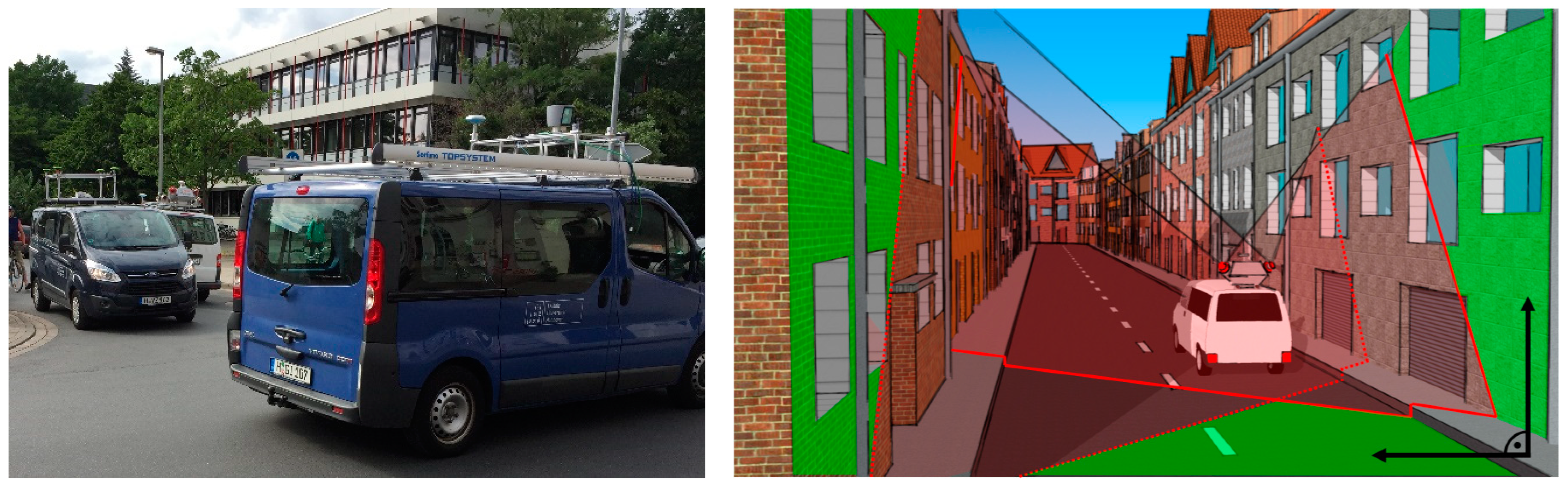
2.1. Experiments and Data

In order to collect data supporting the heterogeneous research topics, collaborative large-scale experiments (see Figure 1) are conducted in regular intervals, emulating the capabilities of automotive sensors of upcoming car generations by equipping real cars with multi-sensor platforms that collect large quantities of data about the environment. As the communication and online-processing capabilities are not in the focus of the project, one of the main goals is to provide a realistic environment in which simulations with real data can be conducted. The range of sensors used in these measurement campaigns include LiDAR systems recording dense 3D point clouds of the environment, stereo cameras for imaging and photogrammetric 3D reconstruction, as well as GNSS/IMU systems for localization. In addition, existing information from maps and 3D building models is also included in the system, which is considered as an additional sensor—a kind of memory of the past states of the environment.

As in any multi-sensor system, sensor data are obtained in each sensor’s coordinate frame. A calibration of all relative positions and orientations between sensors is performed for each experiment to allow a transformation of all measurements into a common frame. This makes a transformation of all sensor data into a global coordinate frame possible, using measurements of the on-board localization sensors to establish a relation between measurements and spatial objects with known global coordinates or between multiple vehicles. This may include vehicle-to-vehicle measurements, vehicle-to-infrastructure measurements, or direct absolute measurement of the geographic location (e.g., with GNSS).

In addition to sensors for localization, information about static and dynamic objects in the environment are continuously recorded: this includes both static objects such as the road surface and buildings as well as dynamic objects such as other vehicles and pedestrians on the road.

Due to the large number of sensors involved and the high spatial and temporal resolution of measurements, these experiments produce large volumes of raw data. During the first large-scale experiment, three vehicles equipped with multi-sensor platforms recorded data for about two hours. During this time, the data collected by three stereo-camera pairs, two laser scanner systems, and ten GNSS/IMU systems amounted to a data acquisition rate of up to 1 GB/sec of raw sensor data. This resulted in a dataset of about 5 TB after decompressing and initial post-processing, before further processing in the context of the individual research projects.

2.2. Challenges and Goals

The diversity and interrelation of the sensors, having different resolutions in space and time with measurements from different domains (point observations/areal observations), observations of static and dynamic elements of the environment, and quality (high and low precision sensors), lead to highly complex datasets. Experiments yield large numbers of separate data logs with sensor-specific data formats across multiple sensor platforms. The unprocessed experimental data represents raw sensor measurements, and it is not yet aligned to be consistent with other observations. This means that geo-referencing may not be optimal and might even be a goal in its own, as most sensor measurements cannot be geo-referenced directly. Instead, a transformation between multiple coordinate systems (applying transformation parameters obtained by sensor-to-sensor calibration) is applied, which ends up at the global positioning sensors with measurements in a global frame. Furthermore, sensor measurements are related to points on the surface of objects (static objects or dynamic objects), whose identification (through segmentation and classification) is part of the research but not part of the measurement.

Thus, sensor data undergoes a gradual transformation process from raw sensor measurements (primary data) through different representations (processed data) with an increasing degree of refinement up to semantic object information (see Figure 2). For dynamic objects, the assignment of a location in space is only applicable for the time instant of the measurement, thus temporal information needs to be stored as well. This way, data encompasses both raw data and enriched data, where “enriched” relates to different aspects, e.g., a transformation to a global coordinate system or an annotation with (light) semantics.

Even though our datasets are mostly used by researchers within the RTG, we face challenges related to research data management on a larger scale: while the participating institutes work in related domains and on a common overarching topic, they have established different ways to represent their data and results that are not immediately compatible with each other. These different communities of domain experts work together in the context of the RTG and must find a common basis in order to share their data and results, in order to avoid introducing additional steps related to understanding and transforming each other’s data representations for each individual data analysis task. In addition, since the RTG is organized in three consecutive cohorts of researchers working on a common dataset, the possibilities to communicate about data personally are limited between members of different cohorts. In these cases, good documentation of the data and its properties are crucial.

On this account, the FAIR data principles can be used to define requirements for the internal research data management. The FAIR data principles demand that research data should be findable and accessible, as well as interoperable and re-usable. This implies the necessity of a structured data storage with automatic search mechanisms on rich metadata (metadata requirements F2, R1.2-3, as well as the infrastructural requirement F4 in [1]). In order to make the complex datasets (including all versions and representations) findable for researchers, search mechanisms have to be provided that allow inspecting the data using spatio-temporal queries on both the data and the associated meta-data, close to the concept data cube [14], or more specifically the space-time cube [15]. Since access to the data is granted to RTG researchers on a file system level, principles A1 and A2 do not apply here. The remaining challenges that the proposed research data management infrastructure tries to solve are related to FAIR data principles I1-3 (interoperability of data representations). Considering these FAIR principles already on the level of internal data storage makes future publications of parts of the data easier. As principles F1, F3, and R1.1 do not directly apply to internally used data, they must be taken into account during the data publication process. This includes the assignment of globally unique identifiers (e.g., in the form of DOIs) and appropriate data usage licenses.

The goal of the research projects is to analyze and further interpret the data. These analysis processes must be applicable to the large datasets; thus, the system is linked to computational hardware for parallel processing. Analysis techniques employed in our research are closely related to the specific types of sensors. Images are processed using image processing algorithms, using, e.g., OpenCV [16] or object recognition using Deep Learning (e.g., TensorFlow [17]), LiDAR data require point-cloud algorithms (e.g., Point Cloud Library [18]). GNSS and IMU data can be coupled for robust trajectory determination. These techniques, among many others, combined with geodetic modeling of the measurement process as well as filtering of measurements from multiple sensors, generate datasets of high complexity (high-dimensional time series data across multiple sensors). Using, e.g., occupancy grids, maps are constructed containing both static features (e.g., geometry of roads and buildings), as well as spatio-temporal information, e.g., in the form of heat-maps containing information about the probability of certain classes of dynamic objects appearing at specific locations in the environment. To this end, individual objects are identified through segmentation and classification of images as well as point clouds. Derived datasets produced by the analyses of these individual research projects are stored in addition to the raw sensor data. This allows more complex analyses in the domain of (real-time) positioning, making use of higher-level knowledge. Examples for derived datasets include corrected versions of datasets (e.g., aligned point clouds), object segmentations, or 3D vehicle models.

On the computational side, the quantity and complexity of data required for individual analysis steps at a time is large, leading to high requirements regarding data transmission and computation in terms of bandwidth and computational power. Therefore, it is essential, that the (large) datasets can be processed with adequate hard- and software, so elements of parallelization are also included in the framework.

Ultimately, the goal is to allow for software reuse by developing and providing software elements [19], which are suitable to be used as a kind of construction kit for collaborative integrity. Software modules will be developed which can be plugged to conventional analysis processes to enhance their capabilities by allowing to quantify integrity. This aspect, however, is beyond the scope of this paper.

3. Related Work

Increasing digitization and novel sensor development and deployment results in more information about our environment and thus potentially leads to more insights into previously unknown interrelations. However, the difficulties in dealing with ever-increasing amounts of data, triggered by the growing number and performance of sensors, which are finding their way into all areas of everyday life, have become an important topic in research in recent years. The vast amount of datasets available for research increasingly requires technical infrastructures for adequately storing the data so that they can be easily found, accessed, integrated, and analyzed.

To facilitate better scientific data publication practice, the domain-independent, high-level FAIR principles (findability, accessibility, interoperability, and reusability) were proposed [1]. These principles require—among others—that the properties of the datasets are stored together with the data in a standardized way that is comprehensible for the machine, and that the data themselves are stored in interoperable data formats. To this end, standards were developed to annotate datasets with metadata (“data about data”). The Resource Description Framework (RDF) developed by the W3C [20] is an XML-based language to encode metadata in a structured, machine-readable way. In terms of useful properties, there have been proposals like the Dublin Core set of metadata items to add details about content, intellectual property, and instantiation of the data [21,22]. In addition, domain-specific standards were established within the different research communities, for example [23,24] for geospatial datasets. An overview over further general and domain-specific standards is available at the website of the Research Data Alliance or on metadata catalog websites [25,26].

Practical applications of the FAIR principles have been developed within individual domains of research, focusing on domain-specific requirements. Typical FAIR applications in the geo-data domain (see [27,28] for an overview) are related to geodata infrastructures (GDI, see [29]): encoding of geo-data into interoperable formats and re-using existing data transformation modules (Web Services) in a decentralized way, allowing geographical data from different sources to be integrated in a common spatial reference frame, using typical geo-information (GIS) operations that are widely applicable to different types of spatial data. These web services can cover data transformation, data integration, or data analysis tasks of varying complexity as well as visualizations of geographic data. Standardization organizations such as the Open Geospatial Consortium (OGC) [30] promote standards for better interoperability, including data formats and interface specifications. For raw sensor data accessible directly through the web, the OGC Sensor Observation Service [31] is a web service standard that defines languages for both sensor self-description (Sensor Model Language [32]) and encoding of sensor measurements (Observation and Measurements [33]).

However, the most common way to make data accessible currently is to publish datasets in public or institutional research data repositories (an overview of data repositories is provided by meta-repositories such as [34]), that support different subsets of data and metadata standards. In addition, data catalog services, e.g., [35] by OSGeo [36], MIT Geodata Repository [37], Pangaea [38], and Harvard Geospatial Library [39], provide direct access to individual, usually domain-specific datasets. So-called metadata harvesting [40] is used to transform between different standards and to integrate all the different standards utilized by repositories and publishing researchers.

4. Proposed Data Storage Solution—System Overview

Storing data in a structured and secure way is a central aspect of data management. The proposed data management system was designed to reflects the size and organizational structure of the project. The goal was to store and make easily accessible raw data as well as derived data, in addition to data documentation in the form of metadata, for a large range of sensors and data types (including LiDAR point clouds, images, as well as GNSS/IMU time-series data). Concerning data inspection, the typical way to query data is via the semantic information (e.g., “give me all data obtained with a specific type of sensor”). Besides this, a natural way to inspect and query spatial data is the spatial domain, i.e., coordinates or bounding boxes (e.g., “show me all images taken at junction X”). In addition, temporal information can be used to search or narrow down a query (e.g., “give me all trajectories which were acquired between 10 a.m. and 1 p.m. between 1 November 2018 and 23 March 2019”).

In this section, the key components of the data storage system are described. As in the RTG project the experiments form a central element, the storage of the data is organized along those conducted experiments, which gives its logical structure. A main element is a visual interface, which allows for easy visualization and inspection of the available data.

The datasets are stored persistently on a single central file server (see Section 4.1). Data are stored in a hierarchical way that reflects the structure of the large-scale experiments (see Section 4.2). A single metadata file is added into each dataset folder (see Section 4.3), where one dataset corresponds to a single set of continuous measurement of a single sensor (i.e., from start to end of recording). As this structure does not support a structured search by custom criteria, a fully automated data crawler (see Section 4.4) is used to browse the current structure of the data folders and represents all datasets with their temporal, spatial, and other metadata in a spatial database. This way, a separation between the logical view on the data (represented as data array) and the physical (hierarchical) storage can be achieved.

In addition to giving direct access to the research data files, the file server acts as host to a graphical web interface (see Section 4.5) that allows project members to visually inspect and compare all datasets in a dynamic, interactive web-map and supports data queries on the spatial metadata database. In order to run computationally expensive computations, the RTG operates a Hadoop (Big Data parallelization framework for large structured datasets, see [41]) cluster consisting of six nodes as well as a GPU server with eight GPUs, mainly used to support the training of networks in the context of Deep Learning (see Section 4.6). Figure 3 gives an overview over the system components and the associated activities for all phases of research data handling in the RTG.

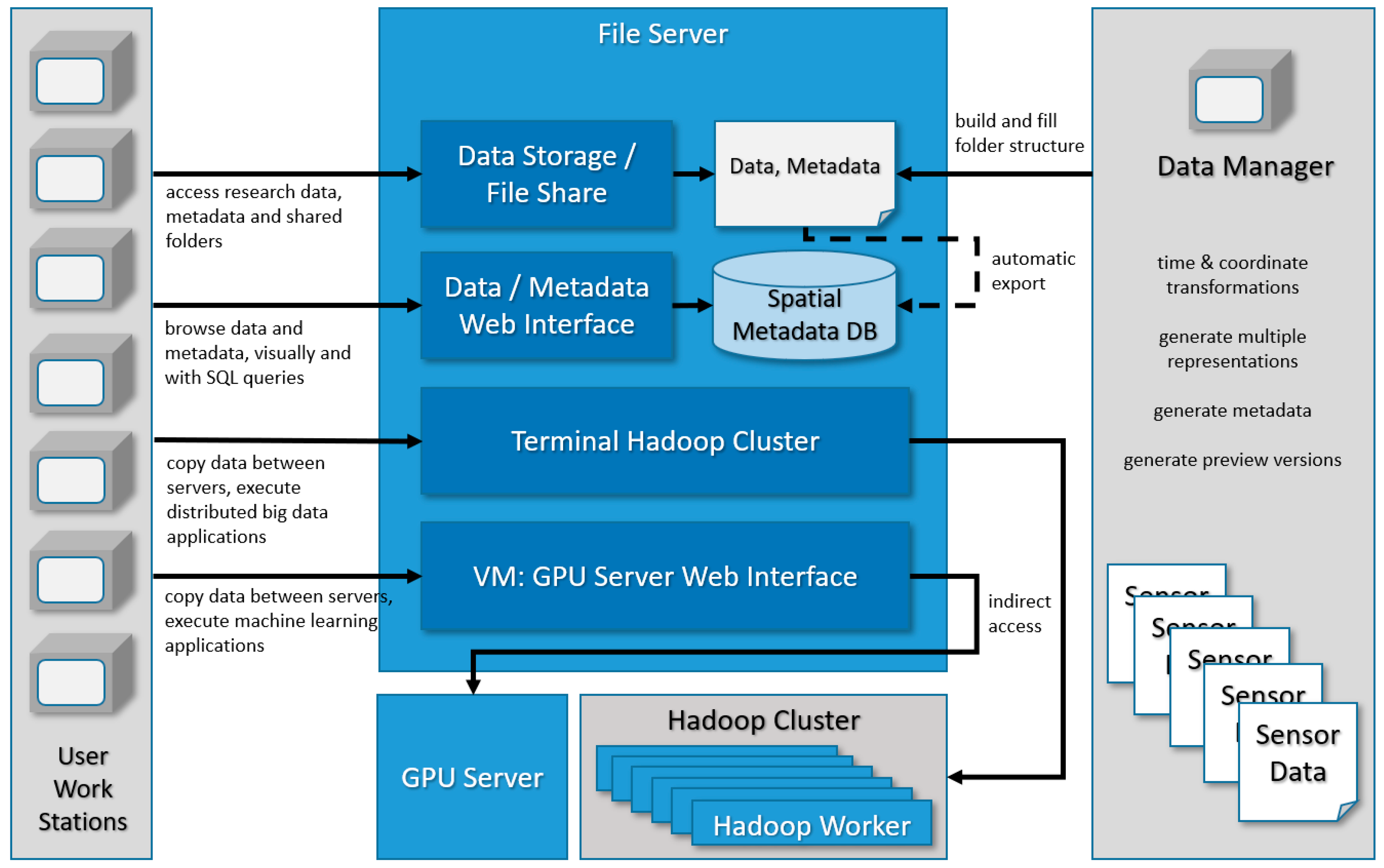
4.1. IT Infrastructure

The RTG operates a central file server in collaboration (server housing and network management services) with Leibniz University’s Department for IT services (LUIS). Data are stored physically on hard drives in a RAID-6 group, currently with a total net capacity of about 60 TB.

The file server acts as single point of access for several project-wide services: file shares are set up to provide access to all datasets for all RTG members on different client operating systems (mainly Win/Linux based). Individual home folders and shared folders for organizational units are realized in the same way, differing in ownership and access rights for different users and user groups.

Computational servers (Hadoop cluster and GPU server) are physically located next to the file server. All servers are connected in an internal 10 Gbit LAN (using Link aggregation to achieve a bandwidth of up to 20 Gbit) to support fast file transfer between the file server and the other cluster nodes, while communication with this cluster from outside is limited to 1 Gbit (for infrastructural reasons). The file server acts as gateway to access the computation clusters (that are otherwise not directly accessible) for uploading and executing the program code as well as giving access to computation results on those machines.

Authorization for all services is managed over an Active Directory (AD), in which users and roles with different access rights are be managed. Login attempts to any of the server’s interfaces (Hadoop Gateway console, web interface, Samba file shares) are delegated to and processed by the AD server. In addition, firewall rules are set up to only allow connections from certain IP ranges related to organizational units within the project, limited to a certain set of ports related to the supported services. Communication is limited to secure/encrypted protocols in all cases, namely SSL/TLS, SSH, HTTPS, and LDAPS.

4.2. Physical Data Storage

On the file system level, each dataset consists of one or multiple files, in some cases with an internal folder structure, depending on sensor type and data format. Each dataset is stored in a separate folder together with the metadata file (see Section 4.3). The granularity of a dataset is chosen depending on the structure of the corresponding experiment such that no further decomposition of the data is possible with respect to the goals of the experiment. For example, a single drive with defined start and end points might constitute an experiment; all datasets gathered along this way will also exist as separate segments corresponding to that drive.

Around those dataset folders on the bottom of the folder hierarchy, a folder structure was created that is suitable for manual browsing by the researchers, mostly driven by the organizational structure of the experiment. Currently, the top-most folder level corresponds to different measurement campaigns, the next level separates mobile platforms/vehicles, the third level separates sensors, and so on. On the bottom levels, different representations of the data are stored, including the original raw data (which are always kept to prevent loss of data during conversion steps) and converted interoperable formats for different purposes (see Section 5.1).

Through the use of the metadata crawler (see Section 4.4), a re-organization of the folder structure is possible at any time without affecting the automatic search, as long as the dataset folders on the bottom level of the folder hierarchy are kept intact.

4.3. Metadata

The term metadata refers to information about datasets. This includes information that cannot be inferred from the data in any way, i.e., information that needs to be explicitly associated with the dataset at the time of data storage. In addition, metadata can also be used to store information that is implicitly contained in the data and can be retrieved with some effort, for example to make explicit information that would otherwise require costly computations to access [42]. For our datasets, a subset of the Dublin Core features [21] was adopted in addition to some custom domain-specific metadata reflecting relations between the data and the experimental setup. This includes nominal and categorical attributes such as ownership/authorship of datasets (equivalent to creator/publisher in Dublin Core) as well as encoding/file format details (format). A generic text field (description) is used to store textual descriptions for future users, containing details about the experiment context or the calibration process.

In addition, domain-specific metadata fields were added to store associations between experiments and sensor platforms or information about sensor types and sensor device IDs. Two metadata fields are used to represent derived spatial and temporal information as a basis for spatio-temporal indexing of the datasets, inspired by the date and coverage metadata fields of the Dublin Core. The temporal interval in which the dataset was obtained (using experiment-wide synchronized, high-accuracy GPS timestamps) is explicitly stored, allowing temporal filtering of datasets. For some sensors, these timestamps are explicitly stored in the data, from which they are retrieved once and then stored as part of the metadata. For sensors that do not explicitly store timestamps, the time interval from other sensors on the same platform recording simultaneously (during data logging) was used. The same principle was applied to the location of sensor observations: localization information from GNSS/IMU systems present on all sensor platforms was transferred and associated with the datasets recorded on the same platform, again to support filtering/searching of datasets by spatial criteria. To this end, minimum bounding rectangles of the GNNS trajectories are stored with each of the datasets, as a more fine-grained spatial resolution (through temporal association of sensor observations with individual GNSS positions) would require further decomposition of the datasets into individual observations. Both of these fields contain only rough values to support spatio-temporal filtering; precise values during analyses need to be directly obtained from the data, depending on the specifics of the analysis.

A template for the metadata file, containing all mandatory metadata fields, is added to each dataset folder in the process of creating the folder structure after an experiment. This template includes comments that define semantics and allowed values (where appropriate) for each metadata field. This metadata file is then filled out by the researchers responsible for each dataset. Automatic checking of the validity of the XML (e.g., against a predefined grammar) is not performed yet but is certainly a feature to consider in the future.

4.4. Spatial Database

In order to allow for a scalable storage and multi-user access, the data are automatically imported into a spatial database (specifically [43]), where all metadata of the datasets are directly accessible for complex queries. It makes use of a script that traverses recursively the full folder structure specifically looking for the presence of a metadata file that denotes datasets. Based on the contents of the metadata file, the script generates database entries for each dataset, including the current storage location of each dataset on the file server. In the process, syntactical errors in the metadata files can be detected. During the database import, datasets are not decomposed further (e.g., into individual measurements), as this would introduce a number of additional challenges: observations are linked to specific measurement processes, introducing measurement errors and interdependencies between multiple sensors during the same experiment, which are themselves a key part of our research.

The database allows SQL queries on arbitrary data properties and their relations (e.g., spatial queries) and simple temporal queries as well as queries on all nominal and categorical metadata that are included in the metadata XML files. This search interface supports use cases such as retrieving all datasets collected at a specific time (e.g., within the same experiment), data observed at the same location (across multiple experiments), or datasets generated by the same sensor (independently of time and location), similar to the operations defined in a data cube [14].

4.5. Web Interface and WebGIS

The file server hosts a website that allows visual inspection of the data and offers filtering and visualization functionalities to the users. The central element of this web interface is a web map that displays preprocessed visualizations for all spatial datasets on top of a general map (e.g., from OSM or mapping agencies), allowing inspection, selection, and comparison of possibly relevant data. In addition to explicitly adding layers related to specific datasets to the map, datasets can be filtered—spatio-temporally or semantically—by adding SQL filter statements into a text field.

Previews of datasets are available as raster tiles and/or as vector data, depending on the type of data at hand. They can be processed and visualized quickly and contain all the necessary information for data selection and visualization (see Figure 4). For dense, spatially distributed data such as point clouds, 2D raster representations (projections to x-y-plane) are preprocessed with multiple LODs/resolutions to support different zoom levels of the web map (i.e., higher levels of detail are revealed when zooming further in without running into trouble on low zoom levels with large to high-resolution tiles). The scripts to produce a full image pyramid of tiles for multiple zoom levels are available, which can customize rendering specifics, i.e., the mapping of the data to pixel colors depending on arbitrary data properties, depending on the required analysis (see Figure 5). This way, each dataset may be associated with multiple, different visualizations.

In order to avoid mixing data and preview data, preview files (i.e., tile sets or vector data files) are placed in a separate folder as part of the web interface files. This folder mirrors the folder structure of the original data to maintain the relation with the corresponding datasets. Previews can be also be generated in a distributed way directly on the Hadoop cluster using a parallelized version of the visualization script. Resulting preview files can be imported into the web map directly from the Hadoop distributed file system (HDFS) of the Hadoop cluster using the WebHDFS REST-API.

In addition to data visualization, the Web interface also allows the inspection of the full datasets through a browser: the data storage folders can be searched manually and datasets can be inspected (if data types are supported directly by the browser, e.g., image data) and downloaded using the https protocol. For convenience, there is also an interface for browsing the contents of the Hadoop cluster file system (HDFS). For point clouds, a WebGL-based point cloud viewer was integrated. Furthermore, it provides interfaces to the metadata database, to inspect the contents of the metadata database and to execute SQL queries on it.

4.6. Hadoop Cluster/GPU Cluster

In order to provide computational capacity for big-data computation tasks, a single GPU server including eight GPUs and a Hadoop cluster consisting of six servers (nodes), are hosted physically right next to the file server to allow a high-bandwidth data connection for fast data transfer. The file server acts as a gateway to upload and run jobs.

The Hadoop cluster runs the latest version of Cloudera distribution including Apache Hadoop (CDH [41]), with installations of distributed services related to the Hadoop ecosystem, including HDFS/YARN, Spark/Spark2, HBase/Hive/Zookeeper. The file server is configured to be an edge node of the cluster configured as gateway for all supported services (HDFS/YARN/Spark, etc.), so that data can be uploaded directly from the file server to the Hadoop distributed file system (HDFS) of the cluster, e.g., to distribute and execute applications. This way, these console-based interfaces are available from the console of the file server. In addition, users have read-only access to the graphical management interface of the Cloudera Manager residing on the Hadoop master node of the cluster to supervise cluster status, resource allocation, and application progress.

In the case of the GPU cluster, the file server runs a separate virtual machine hosting DC/OS [44], a distributed operation system based on the Apache Mesos distributed systems kernel. It manages the GPU cluster resources in a single graphical interface, allowing deployment of distributed applications, including resource allocation/management for multiple concurrent users. This graphical interface is available for cluster users under a separate IP and URL in a browser. Computation results from both clusters are immediately accessible: the GPU cluster writes back results directly to the file server, while the Hadoop cluster stores results in the HDFS, which can be accessed like a normal file system from the file server console.

5. Data Management

This section describes the processes developed for preparing experimental data for data storage in Section 5.1, followed by examples for these preprocessing steps in Section 5.2 and examples for the benefits the system provides when working with stored data in Section 5.3.

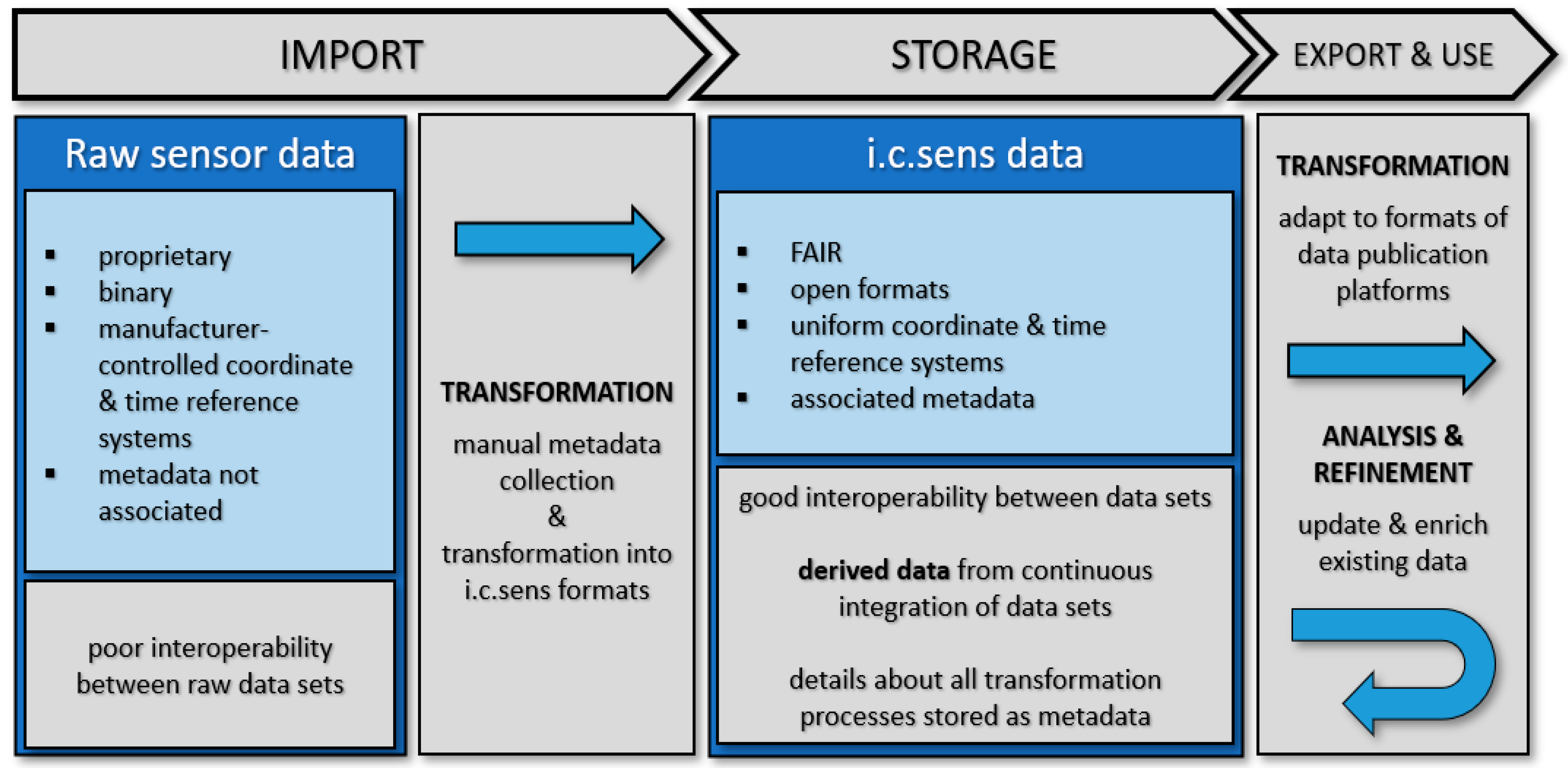
5.1. Data Preparation and Post-Processing

In the context of physical data storage, processes to maintain consistency and integrity within and across all datasets were established. As a safeguard against errors in any post-processing or transformation processes, all datasets are redundantly stored in their original format. However, depending on the sensor and the available data formats, this might result in proprietary data formats that are only accessible using sensor specific soft- or hardware, making them impractical within a large-scale project across organizational research units. In addition, internally used spatial reference systems and/or representation of time measurements might differ across sensors.

Thus, all datasets are transformed into open interoperable formats with unified spatial reference systems (specifically ETRS89/UTM zone 32N, since this is the output format of multiple sensor systems used in our experiments) and time representation (Unix time, since data logging and time synchronization in our experiments use the Robot Operating System (ROS [45]) on Linux machines) that allow both interoperability as well as compatibility of spatial/temporal measurements between all datasets. Specifically, stereo image sequences are stored as separate sequences of PNG images for each camera, with a separate ASCII table including a mapping between image IDs and timestamps; ASCII PLY format is used for point cloud data, RINEX format for GNSS data, most other types of sensor output are stored in CSV format. The transformations into those formats are performed by scripts developed for each type of raw sensor output format.

After successful data transformation metadata are collected and/or computed from the data and manually added to the metadata document (one for each version of each dataset). The metadata document is then placed into the folder of the dataset (see Section 4.3). The folder structure for experiment is built manually, following a fixed order of subdivision (see Section 4.2); all dataset folders are then placed on the bottom level of this folder hierarchy. The top-level of the folder hierarchy for the experiment contains documentation related to the experiment, planning documents, and details about the sensor platforms (including calibration information: sensor-to-sensor and sensor-to-vehicle). Calibration data for individual sensors are placed in the respective sensor folders (some levels above individual dataset level).

Once the folder structure is established and all metadata files are complete, a crawler script is executed which transfers the current state of the folder hierarchy of the file server into the metadata database (see Section 4.4). The database links the current storage locations of the individual datasets with their respective metadata, allowing a server-wide search for these registered datasets by keywords and values from metadata fields.

As a last step of the data preparation, preview versions for each dataset (e.g., raster tiles to use as overlay on a web map or a down-sampled vector-representation) are produced using the previously described sensor type-specific scripts. Preview files are placed in a folder accessible by the web interface from where they are automatically integrated into the web map (see Section 4.5).

5.2. Data Ingestion Example

In the following section, the practical implications of the steps from Section 5.1 are illustrated by taking a closer look at the data produced by the multi-sensor configuration of a car used in one of our experiments, highlighting some challenges encountered in the process. Technical details irrelevant in the context of the process are omitted.

The car is equipped with a RIEGL VMX-250 Mobile Mapping System (MMS), including two RIEGL VQ-250 2D Laser Scanners, four cameras (used for point cloud coloring), a GNSS/IMU, and a computer with proprietary software logs the measurements from these sensors. Output of the sensor is a complex project folder using proprietary file formats, requiring proprietary software to extract various sensor outputs, including solutions for the GNSS trajectory and (colored) point clouds, either in sensor coordinates or in world coordinates. In addition, a pair of stereo cameras was attached to the front of the car roof and a separate GNSS/IMU system, as the MMS does not give access to the raw GNSS data, unfortunately. Data from the stereo camera and from the GNSS/IMU system are logged using ROS nodes on a Linux system; in the process, GPS timestamps from the GNSS sensor are associated with the stereo images. The MMS logs to a different computer, using GPS timestamps as well. However, both GNSS systems use different spatial reference systems.

The different sensors on the car produce the following raw data formats: a large folder with a complex internal structure for the MMS data and so-called ROS bags logged by ROS, which contain timestamped messages (organized in so-called ROS topics) from the recording. These raw (or first) logs of the data are stored on the file server. As these formats are not directly useable by all researchers, they are transformed into interoperable formats (lossless binary standard formats for image data and well-defined ASCII text formats for GNSS and LiDAR data). For the MMS projects, the proprietary MMS software is used to derive the required data (e.g., an ASCII representation of the GNSS trajectory and the colored, full-resolution point cloud in world coordinates). For the ROS bags, the messages are exported as a single ASCII text file for the GNSS/IMU system (using sensor-specific formatting) and a folder with stereo image pairs (PNG format) with associated GPS timestamps in an ASCII text file.

In addition, a post-processing step is performed for all of the exported versions of the data, during which timestamps and spatial coordinates of all sensor data are transformed into the common representations, using format-specific scripts to automatize the transformation. This later allows our researchers to work with the prepared datasets without having to deal with coordinate and timestamp transformations themselves. Having unified timestamps and spatial coordinate reference systems makes it easily possible to export the data automatically into other formats.

For each dataset, including different versions or formats of the same dataset, a metadata XML file is created as a copy of a predefined XML template. It contains metadata fields identified as useful in the context of our research, including sensorType, sensorName, dataFormat, sensorID, experimentID, sensorPlatformID, timeInterval, spatialBoundaries, owner as well as a free-text description field for further unstructured details/comments. Some of these fields are required for certain functionalities; for example, these fields are contained in the metadata database and are thus available in SQL queries on the metadata. Arbitrary additional fields can be defined when filling the metadata; these are, however, not used by any automated processes. Metadata files are edited by the “owners” of the respective sensors, i.e., in most cases, the researchers who contributed the sensor hardware and software to the sensor platform. To reduce the risk of entry errors, predefined lists of expected values are defined in the metadata XML template for some metadata fields, e.g., the metadata field sensorType may only have values such as STEREO_CAMERA, LASER_SCANNER, GNSS, etc. Data-format-specific scripts assist in calculating the time interval and spatial boundaries for all datasets, as these values are integral part of the metadata, as they support (approximate) spatio-temporal queries in the metadata database. For sensors without self-localization capabilities (e.g., stereo cameras), the spatial boundaries of the data from one of the GNSS sensors on the same sensor platform are used. Of course, there is some redundancy among metadata files, as the same original dataset might be stored in multiple export formats.

Once all datasets have been transformed into their final formats, a folder structure is created on the server that supports manual search. To this end, relations between datasets resulting from the experiment design are reflected in the folder hierarchy, following a structure as follows:

EXPERIMENT_ID > SENSOR_PLATFORM_ID > SENSOR_TYPE > SENSOR_ID > DATA_FORMAT > datasets

For the specific sensor platform from the example this would result in the folder structure shown in

Table 1. Possible folder structure for data obtained with the sensor platform described in Section 5.2.

EXPERIMENT_1
	SENSOR_PLATFORM_1
		PLATFORM_CALIBRATION_DATA: includes data from platform calibration, i.e., raw measurements and obtained transformations between sensors
		ROS_BAGS: storage for raw version of data logged by the ROS computer (includes data from stereo camera and GNSS/IMU system) as ROS bags; useable to re-create the sensor data traffic during recording
		MMS
			FULL_PROJECT: proprietary MMS storage format can be used by proprietary software to export various types of MMS-related data; this is considered the raw data for the MMS; metadata XML file
			EXPORTED_POINT_CLOUD: point cloud data in various formats, e.g., colored point cloud with absolute coordinates separated into uniform spatial grid cells to reduce file size, full (down-sampled) point cloud; metadata XML file
			EXPORTED_TRAJECTORY: export from MMS-internal GNSS as ASCII text file; metadata XML file
		STEREO_CAMERA
			STEREO_CAMERA_1
				CAMERA_CALIBRATION_DATA: data from camera calibration, i.e., raw images and obtained (intrinsic) camera parameters
				IMAGE_DATA: includes pairs of left/right images and an ASCII table that maps timestamps to image IDs; metadata XML file
		GNSS/IMU
			GNSS/IMU_1
				PROPRIETARY_FORMAT: original sensor-dependent format, in some cases, only useable using sensor-specific proprietary software; metadata XML file
				EXPORTED_FORMAT: export to accessible, interoperable ASCII format after export from the proprietary format using proprietary software; metadata XML file

.

Bold folder names designate structuring folders by categories. Italic folder names are the bottom-level folders containing the actual datasets as well as the individual metadata files. Underlined folder names have calibration data required for integrating and interpreting the respective datasets. Some of the bold folder names mirror metadata attributes, making explicit data properties on the file system level to support manual search processes. The folder names are assigned manually and are neither strictly enforced nor used by automated search processes. In fact, since the metadata files are part of the corresponding dataset folder, folders above in the hierarchy can be re-structured arbitrarily without impeding automatic search capabilities.

At this point, a crawler script is manually executed, which traverses the file server folder hierarchy. Whenever a metadata XML file is encountered, its contents (values of predefined fields) as well as its location (which is always a dataset folder) are stored in the spatial database. For the example data, the database now contains seven entries: one for the raw ROS bags, one for the raw MMS data, the two MMS exports, the stereo camera dataset and the two GNSS datasets.

As a final step after storing the data, preview versions for each dataset are prepared that can then be displayed in the web map of the web interface; if a dataset is available in multiple formats, only a single preview is produced. For the point clouds, raster images (tiles) are created by rendering code with customizable resolution and visualization. These tiles are later displayed directly on top of the web map’s base map (see Figure 4). For the MMS and GNSS trajectories, vector representations are more suitable. To this end, heavily sub-sampled versions of the original trajectories are produced, which are later displayed as polylines on top of the web map (see Figure 5, right). There is currently no preview functionality for stereo camera images. The preview files are kept in a separate folder structure, mirroring the data folder structure to avoid mixing data and their representation, while making the relation between the original data and the preview data explicit.

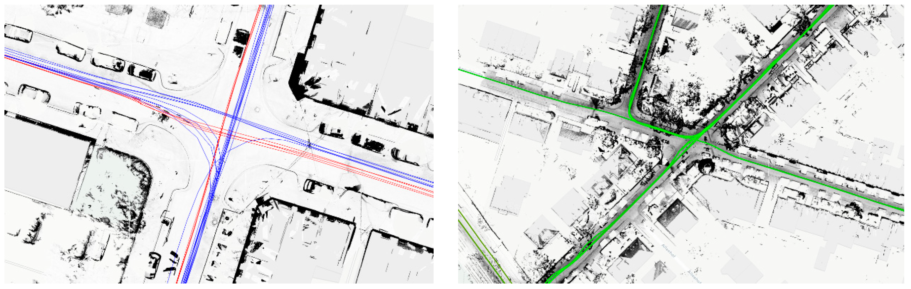
5.3. Data Usage Examples

This section briefly describes real data integration tasks that make use of multiple datasets from a single experiment using the sensor setup described in Section 4.2, illustrating how the data management system supports the preparation and execution of the necessary steps.

Example 1:

Assume that a researcher wants to detect traffic signs in a point cloud around a junction. This could simply be solved by checking the color of the 3D points and applying a semantic segmentation. As the point clouds do not contain color values, the color of the 3D points must be obtained from image data first, which is also available in the system. The projection of 3D LiDAR points into 2D images to retrieve the correct color values requires a series of transformations between multiple global or sensor-centric coordinate systems based on the LiDAR point cloud in absolute coordinates, the intrinsic camera parameters (from camera calibration), the absolute pose of the sensor platform from the GNSS-IMU system as well as the (static) transformation between the GNSS coordinate system and the camera coordinate system (from sensor-to-sensor calibration). The result of this transformation is a set of 2D image coordinates corresponding to the 3D points measured by the LiDAR sensor, from which the color values can be retrieved and assigned to the 3D points.

The data management system supports the task in a multitude of ways. The data exploration interface using the metadata database and/or the web map gives the researcher a means to inspect the data beforehand. Using the visual interface, the researcher can inspect which LiDAR data and which image data are available at that junction. In addition, the datasets on the file server can be filtered for data related to the specific car, experiment, and sensors using SQL queries. Furthermore, spatial and temporal constraints can be added to narrow down the search. This also gives direct access to the associated metadata and documentation of the experiment. The required calibration data are available in the folders related to that specific experiment/vehicle combination (sensor-to-sensor platform calibration) or in the individual sensor folders (sensor calibration), respectively.

Depending on the workflow at hand, the found datasets can then be downloaded to the researcher’s workstation (using the Samba file shares) or into the HDFS of the Hadoop cluster (using the Hadoop console interface) for further processing. In the latter case, the (Hadoop-specific) transformational code needs to be uploaded into the HDFS as well. Results of the transformation can be copied back to the file server using the same interfaces.

Example 2:

Another example is a researcher who wants to use in his vision-based system for other traffic participants (cars, pedestrians) as “mobile ground control points”. This requires that the data management system provides data, including images and poses of other cars and pedestrians, obtained from analyses in the context of our research topics. To this end, analysis results from individual research work are uploaded to the fileserver as derived datasets. As all datasets are registered in the same coordinate system and all the necessary information (position, orientation, calibration of camera) is available, the task then reduces to selecting the objects that are visible in each image, respectively.

6. Summary and Future Work

In this paper, we presented an implementation of a research data management system that features structured data storage for spatio-temporal experimental data, including metadata management and interfaces for visualization and parallel processing. We described in detail the organization of our storage and computational hardware as well as structures and processes related to data collection, preparation, and storage and demonstrated the association of data with metadata, resulting in a fully searchable database. Finally, we gave practical examples for the handling of real datasets, i.e., required data preparation steps for data storage as well as benefits when using the data in the context of real scientific tasks.

Our research domain is challenging, as the observation of highly dynamic environments using dynamic sensor platforms leads to high interdependencies between sensor calibration, self-localization, sensor measurements, and time synchronization between sensors. This complexity is difficult to handle with out-of-the-box data storage solutions. With the presented approach, some of the representational problems related to these challenges could be overcome. Adhering to the FAIR principle, all datasets are stored as open, interoperable formats. In this context, uniform time and spatial formats are used, allowing direct integration of all datasets. Calibration data (from sensor platform calibration and sensor calibration) are explicitly stored in a logical manner relative to the datasets.

While working with the described research data management system, some possible improvements were identified that we plan to employ in the future. This includes improvements in some of the standard workflows, such as the editing of metadata, which could use a bulk-editing operator (adding the same metadata field/values to a number of datasets at the same time, reducing the need for manual copying and pasting). We also want to support automatic exports of our metadata files into different metadata standards commonly used by research data repositories (see [25,26]) to support and facilitate the data publication process.

In terms of additional functionalities, interdependencies between datasets could be modeled better; this encompasses cross-references (using unique dataset IDs) between datasets via metadata, realizing versioning of datasets. Each dataset would then refer to the dataset(s) it was created from, ideally also with a reference to the code it was created with, i.e., encoding the relation “dataset B was created from dataset A using transformation software T” in the metadata files. In the same way, the relation between sensors or sensor platforms and their calibration data can be stored as metadata.

Another next step is to decompose existing datasets and, in terms of data granularity, go from the level of full experiments to the level of individual observations. For example, instead of storing full point cloud datasets, individual point observations could be stored. This would allow the spatial database to create new complex datasets from spatial queries, e.g., returning all the 3D points measured in a defined spatial area across multiple point clouds. On the database level, this kind of decomposition does not lead to any new challenges. However, the complexity of such a solution increases greatly, as all the information about the origins (e.g., properties of and interdependencies within the corresponding experiment/original point cloud, including quality measures and positional accuracies) of each point needs to be preserved as part of the output.

References

1. Wilkinson, M.D.; Dumontier, M.; Aalbersberg, I.J.; Appleton, G.; Axton, M.; Baak, A.; Blomberg, N.; Boiten, J.-W.; de Silva Santos, L.B.; Bourne, P.E.; et al. The FAIR Guiding Principles for scientific data management and stewardship. Sci. Data 2016, 3, 1–9. [Google Scholar] [CrossRef] [PubMed] [Green Version]
2. Schön, S.; Brenner, C.; Alkhatib, H.; Coenen, M.; Dbouk, H.; Garcia-Fernandez, N.; Kuntzsch, C.; Heipke, C.; Lohmann, K.; Neumann, I.; et al. Integrity and Collaboration in Dynamic Sensor Networks. Sensors 2018, 18, 2400. [Google Scholar] [CrossRef] [PubMed] [Green Version]
3. Principles for the Handling of Research Data. Available online: https://www.mpg.de/230783/Principles_Research_Data_2010.pdf (accessed on 18 August 2020).
4. Kaplan, E.D.; Hegarty, C.J. Understanding GPS/GNSS: Principles and Applications, 3rd ed.; Artech House: London, UK, 2017. [Google Scholar]
5. Reid, T.G.; Houts, S.E.; Cammarata, R.; Mills, G.; Agarwal, S.; Vora, A.; Pandey, G. Localization requirements for autonomous vehicles. SAE Int. J. Connect. Autom. Veh. 2019, 2, 173–190. [Google Scholar] [CrossRef] [Green Version]
6. Schön, S. Integrity—A Topic for Photogrammetry? In The International Archives of the Photogrammetry, Remote Sensing and Spatial Information Sciences XLIII-B1-2020, Proceedings of the XXIV ISPRS Congress, Virtual Event, 31 August–2 September 2020; Copernicus GmbH: Göttingen, Germany, 2020; pp. 565–571. [Google Scholar]
7. Voges, R.; Wieghardt, C.S.; Wagner, B. Finding Timestamp Offsets for a Multi-Sensor System Using Sensor Observations. Photogramm. Eng. Remote Sens. 2018, 84, 357–366. [Google Scholar] [CrossRef]
8. Dbouk, H.; Schön, S. Reliability and Integrity Measures of GPS Positioning via Geometrical Constraints. In Proceedings of the 2019 International Technical Meeting of The Institute of Navigation, Reston, Virginia, 28–31 January 2019; pp. 730–743. [Google Scholar]
9. Garcia Fernandez, N.; Schön, S. Optimizing Sensor Combinations and Processing Parameters in Dynamic Sensor Networks. In Proceedings of the 32nd International Technical Meeting of the Satellite Division of The Institute of Navigation (ION GNSS+ 2019), Miami, FL, USA, 16–20 September 2019; pp. 2048–2062. [Google Scholar]
10. Schachtschneider, J.; Schlichting, A.; Brenner, C. Assessing Temporal Behavior in LiDAR Point Clouds of Urban Environments. Int. Arch. Photogramm. Remote Sens. Spatial Inf. Sci. 2017, XLII-1/W1, 543–550. [Google Scholar] [CrossRef] [Green Version]
11. Peters, T.; Brenner, C. Conditional Adversarial Networks for Multimodal Photo-Realistic Point Cloud Rendering. PFG 2020, 88, 257–269. [Google Scholar] [CrossRef]
12. Coenen, M.; Rottensteiner, F.; Heipke, C. Precise vehicle reconstruction for autonomous driving applications. ISPRS Ann. Photogramm. Remote Sens. Spatial Inf. Sci. 2019, IV-2/W5, 21–28. [Google Scholar] [CrossRef] [Green Version]
13. Nguyen, U.; Rottensteiner, F.; Heipke, C. Confidence-aware pedestrian tracking using a stereo camera. ISPRS Ann. Photogramm. Remote Sens. Spatial Inf. Sci. 2019, IV-2/W5, 53–60. [Google Scholar] [CrossRef] [Green Version]
14. Gray, J.; Chaudhuri, S.; Bosworth, A.; Layman, A.; Reichart, D.; Venkatrao, M.; Pellow, F.; Pirahesh, H. Datacube: A relational aggregation operator generalizing group-by, cross-tab and sub-totals. In Proceedings of the 12th International Conference on Data Engineering, New Orleans, LA, USA, 26 February–1 March 1996; pp. 152–159. [Google Scholar]
15. Kraak, M.-J. The space-time cube revisited from a geovisualization perspective. In Proceedings of the 21st International Cartographic Conference, Durban, South Africa, 10–16 August 2003; pp. 1988–1995. [Google Scholar]
16. OpenCV. Available online: https://opencv.org/ (accessed on 18 August 2020).
17. TensorFlow. Available online: https://www.tensorflow.org/ (accessed on 18 August 2020).
18. Point Cloud Library. Available online: http://pointclouds.org/ (accessed on 18 August 2020).
19. Konkol, M.; Kray, C. In-depth examination of spatiotemporal figures in open reproducible research. Cartogr. Geogr. Inf. Sci. 2018, 46, 412–427. [Google Scholar] [CrossRef] [Green Version]
20. Miller, E. An introduction to the resource description framework. Bull. Am. Soc. Inf. Sci. 1998, 25, 15–19. [Google Scholar]
21. Weibel, S. The Dublin Core: A simple content description model for electronic resources. Bull. Am. Soc. Inf. Sci. Technol. 1997, 24, 9–11. [Google Scholar] [CrossRef]
22. Dublin Core Metadata for Resource Discovery. Available online: https://tools.ietf.org/html/rfc2413 (accessed on 18 August 2020).
23. ISO 19115-1:2014: Geographic Information—Metadata—Part1: Fundamentals. Available online: https://www.iso.org/standard/53798.html (accessed on 18 August 2020).
24. Geospatial Metadata Standards and Guidelines. Available online: https://www.fgdc.gov/metadata/geospatial-metadata-standards/ (accessed on 18 August 2020).
25. Metadata Directory. Available online: https://rd-alliance.github.io/metadata-directory/standards/ (accessed on 18 August 2020).
26. List of Metadata Standards. Available online: http://www.dcc.ac.uk/resources/metadata-standards/list/ (accessed on 18 August 2020).
27. Coetzee, S.; Ivánová, I.; Mitasova, H.; Brovelli, M.A. Open Geospatial Software and Data: A Review of the Current State and A Perspective into the Future. ISPRS Int. J. Geo-Inf. 2020, 9, 90. [Google Scholar] [CrossRef] [Green Version]
28. Breunig, M.; Bradley, P.E.; Jahn, M.; Kuper, P.; Mazroob, N.; Rösch, N.; Al-Doori, M.; Stefanakis, E.; Jadidi, M. Geospatial Data Management Research: Progress and Future Directions. ISPRS Int. J. Geo-Inf. 2020, 9, 95. [Google Scholar] [CrossRef] [Green Version]
29. Bernard, L.; Brauner, J.; Mäs, S.; Wiemann, S. Geodateninfrastrukturen. In Geoinformatik; Sester, M., Ed.; Springer Spektrum: Berlin, Germany, 2019; pp. 91–122. [Google Scholar]
30. OGC. Available online: https://www.ogc.org/ (accessed on 18 August 2020).
31. Sensor Observation Service. Available online: https://www.opengeospatial.org/standards/sos/ (accessed on 18 August 2020).
32. Sensor Model Language (SensorML). Available online: https://www.ogc.org/standards/sensorml/ (accessed on 18 August 2020).
33. ISO 19156:2011. Available online: https://www.iso.org/standard/32574.html (accessed on 18 August 2020).
34. Registry of Research Data Repositories. Available online: http://re3data.org/ (accessed on 18 August 2020).
35. GeoNetwork. Available online: https://www.osgeo.org/projects/geonetwork/ (accessed on 18 August 2020).
36. OSGeo. Available online: https://www.osgeo.org/ (accessed on 18 August 2020).
37. MIT Geodata Repository. Available online: https://libguides.mit.edu/gis/Geodata/ (accessed on 18 August 2020).
38. PANGAEA. Available online: https://www.pangaea.de/ (accessed on 18 August 2020).
39. Harvard Geospatial Library. Available online: http://hgl.harvard.edu:8080/opengeoportal/ (accessed on 18 August 2020).
40. The Open Archives Initiative Protocol for Metadata Harvesting. Available online: http://www.openarchives.org/OAI/openarchivesprotocol.html (accessed on 18 August 2020).
41. Apache Hadoop. Available online: https://hadoop.apache.org/ (accessed on 18 August 2020).
42. Heinzle, F.; Anders, K.H.; Sester, M. Pattern recognition in road networks on the example of circular road detection. In Proceedings of the 4th International Conference on Geographic Information Science, Münster, Germany, 20–23 September 2006; Springer: Berlin/Heidelberg, Germany, 2006; pp. 153–167. [Google Scholar]
43. PostGIS. Available online: https://postgis.net/ (accessed on 18 August 2020).
44. DC/OS. Available online: https://dcos.io/ (accessed on 18 August 2020).
45. ROS. Available online: https://www.ros.org/ (accessed on 18 August 2020).
Figure 1. (left) Photograph of a typical situation during our experiments: in the first Meet and Greet scenario, all three cars meet at a junction. (right) Sensors are attached to moving sensor platforms (vehicles), i.e., sets of sensors are spatially bound to a common frame, which itself is moving through a global frame.
Ijgi 09 00626 g001
Figure 2. Transformation process of raw sensor data into uniform formats supports continuous data integration in the research project and allows simple interfaces for data inspection, analysis, and visualization.
Ijgi 09 00626 g002
Figure 3. Overview of the components of the research data management system, including interfaces and processes associated with different roles within the research training group (RTG). Raw, unstructured sensor data and its metadata are uploaded to the server by the individual researchers. The transformation into unified data formats and the import of data and metadata into the structured data storage are organized by the data manager.
Ijgi 09 00626 g003
Figure 4. Screenshots from the web interface: preview of two trajectories from different vehicles (colored differently) and a point cloud on top of the web map. The renderer for the point cloud visualization is optimized to highlight vertical structures.
Ijgi 09 00626 g004
Figure 5. Additional functions of the web interface: (left:) bounding boxes (from the metadata based on global navigation satellite system (GNSS) sensors on the same sensor platform) shown in addition to the trajectories/point clouds. In this example, the point cloud renderer shows all points and local point density; (right:) trajectory of vehicle, colored by a single feature (speed).
Ijgi 09 00626 g005