Article

Detecting Intra-Urban Housing Market Spillover through a Spatial Markov Chain Model

1
School of Finance, Zhejiang University of Finance and Economics, Hangzhou 310018, China
2
National School of Development, Southeast University, Nanjing 210000, China
3
Department of Informatics, New Jersey Institute of Technology, Newark, NJ 07102, USA
4
Department of Information Engineering, China University of Geosciences, Wuhan 430074, China
5
School of Economics & Management, Guangxi Normal University, Guilin 541004, China
*
Author to whom correspondence should be addressed.
ISPRS Int. J. Geo-Inf. 2020, 9(1), 56; https://doi.org/10.3390/ijgi9010056
Submission received: 29 November 2019 / Revised: 13 January 2020 / Accepted: 14 January 2020 / Published: 19 January 2020
(This article belongs to the Special Issue Geospatial Methods in Social and Behavioral Sciences)

Abstract

:
This study analyzed the spillovers among intra-urban housing submarkets in Beijing, China. Intra-urban spillover imposes a methodological challenge for housing studies from the spatial and temporal perspectives. Unlike the inter-urban spillover, the range of every submarket is not naturally defined; therefore, it is impossible to evaluate the intra-urban spillover by standard time-series models. Instead, we formulated the spillover effect as a Markov chain procedure. The constrained clustering technique was applied to identify the submarkets as the hidden states of Markov chain and estimate the transition matrix. Using a day-by-day transaction dataset of second-hand apartments in Beijing during 2011–2017, we detected 16 submarkets/regions and the spillover effect among these regions. The highest transition probability appeared in the overlapped region of urban core and Tongzhou district. This observation reflects the impact of urban planning proposal initiated since early 2012. In addition to the policy consequences, we analyzed a variety of spillover “types” through regression analysis. The latter showed that the “ripple” form of spillover is not dominant at the intra-urban level. Other types, such as the spillover due to the existence of price depressed regions, play major roles. This observation reveals the complexity of intra-urban spillover dynamics and its distinct driving-force compared to the inter-urban spillover.

1. Introduction

The externalities and spillover effect in housing markets have attracted growing scholarly interest [1,2,3,4,5,6,7]. Extensive studies have been reported for the housing markets in the developed world [8,9,10,11], while developing countries have also begun to pay attention [7,12,13,14,15]. Meen [16] provides convincing economic explanations for the driving forces of spillover and summarizes four major mechanisms by which the housing price spillover can occur: migration, equity transfer, spatial arbitrage, and spatial patterns. Many empirical studies have examined the four mechanisms in the setting of inter-urban spillover [8,9,10,11,13,17,18,19,20,21,22,23,24,25]. Most studies support the mechanisms, such as the spatial arbitrage and spatial patterns, which generate the “ripple”-form spillover with the spatial continuous pattern. While little evidence could support the migration and equity transfer mechanisms, they can potentially lead to the spillover with spatially discontinuous pattern.
The spillover mechanisms documented in [16] are applicable to both intra and inter-urban spillovers, but most studies are on the latter, despite a few exceptions [26,27]. The intra-urban spillover occurs quite differently from its inter-urban analogue. First, spillover within cities allows discontinuity and does not have to be equipped with “ripple” form. This is because within-city relocation is relatively cheap due to the emergence of rapid commuting tools, such as rapid transit buses and metro rail transit. Cheap commuting makes the migration a feasible mechanism to drive housing price spillover; one such example is the reversed urbanization process, which reduced the attractiveness of living close to one’s workplace and lifted up housing prices in surburban areas [28,29,30]. Consequently, spillover is allowed to occur between two relatively distant locations, and thus displays discontinuity [31].
On the other hand, intra-urban spillover cannot arbitrarily occur everywhere. Instead, many other types of spatial segregation that can still restrict spillover continue to function, such as the neighborhood segregation induced by the differences in race [32], education level [33], wealth, and income [34,35], and the possible discrimination between native and migrant residents [33]. Apart from the socioeconomic segregation listed above, urban development and renewal initiatives and housing market intervention policies can also alter the trend of intra-urban spillover [36,37,38]. Finally, market sentiment inspired by various policies does play a role in affecting the range and strength of spillover [25,39,40]. All these competitive forces make the intra-urban spillover a complicated, dynamic system; the direction and boundaries of spillover cannot be so simply predicted as in the inter-urban case, which makes intra-urban spillover deserve a thorough investigation, even if it is not yet receiving sufficient attention in the existing literature.
The intra-urban spillover also differs from its inter-urban analogue in terms of the methodology need. The widely used vector auto-regressive (VAR) model [27,41,42,43] in the inter-urban spillover is not sufficient to analyze the intra-urban spillover. VAR models are designed to capture the dynamic dependence of a sequence of finite dimensional random vectors. Regarding inter-urban spillovers, the housing market in every city can be naturally abstracted as a finite-dimension random vector with its value as the city-level average price. This abstraction is valid because of the stratified network structure displayed in the inter-urban spillover. In fact, spillover effect can always be modeled as occurring through a network, in which nodes represent places among which spillover can happen. Edges describe the existence of economic/geographic connections between their end nodes; these connections form the media for spillover to happen. Because cities are usually distant from each other, the strength of economic/geographic connections is much weaker for places between two distant cities than within the same city. Therefore, the spillover network can always be stratified into two levels. The lower level includes a family of disjoint sub-networks each of which consists of nodes and edges within a city; the higher level is another network with its nodes representing cities and edges being connections among cities. Apparently, if our focus is on the inter-urban spillover, only the high level network is needed, which usually has a relatively small amount of nodes and can be embedded into a finite-(low-)dimensional VAR model [41]. However, for the intra-urban spillover within a city, only a sub-network at the low level is needed. For such a within-city network, due to the lack of geographic isolation, there is not a clear division of nodes and edges into a small amount of disjoint groups in terms of the strength of connections. Consequently, the intra-urban spillover forms an infinite and irreducible network, so VAR models are not applicable due to the lack of limitation.
Other than VAR models, there are many other (spatial-) regression-based methods with which to analyze the intra-urban spatial correlations of housing prices [44,45,46,47] (which are closely related to the intra-urban spillover studied in this paper). Methods in this class always set up a cut-off value for the range of distance only within which spillover can occur [44,45]. The methods are useful in terms of detecting the existence of the “ripple-form” spillover and/or evaluating its scale and significance. But on the other hand, the cut-off value restricts the range of analysis. Only the spillover within the predefined neighborhood can be analyzed; it excludes the possibility of the other types of spillover, such as the co-movement of housing prices across different locations that are not covered by the predefined neighborhood. More critically, due to the restriction within fixed neighborhoods, the spatial dimension of spillover is degenerated. It is represented as a dummy variable; namely, whether or not a spatial structure in the neighborhood, such as the direction and geographic range of spillover, is completely lost. In reality, this type of structural information is often more important than the quantitative scale. Finally, Markov chain models are also used in the study of housing market spillover and the other types of housing market dynamics, such as in [8,10,14,48], among which the Markov-switching model is applied most frequently. It applies particularly to the housing price fluctuations and spillovers induced by the economic boom or recession. The Markov-switching model highlights more on the temporal dependence rather than the spatial dependence of housing price. Although the spatial correlation of housing prices can be added into the framework through inserting the Markovian regime switch into a spatial regression equation [10], the resulting model separates the space from the time, and neglects the interaction between the spatial dimension and the temporal dimension, which, however, is most critical to interpreting the housing market spillover.
To fill the gap discussed above, we integrated a modified version of the constrained k-means clustering method [49,50,51,52,53] and the spatial Makarov chain model to study the intra-urban housing price spillover. Different from the Markov-switching model, a novel combination of the Markov chain model with the time series of housing price is proposed to capture the dynamics behind spillover; the constrained clustering is utilized to search for the most proper set-up for the Markov chain. The proposed method was applied to a data sample consisting of 120,618 housing transaction records (the variables include price, transaction time, and the location of every transacted housing units) in Beijing, China, from October 2011 to October 2017. The data were collected from fang.com, the largest and most well-known online platform that provides detailed transaction information of second-hand apartments in China. After analysis, we found that in the housing market of Beijing, there are 16 robust housing submarkets among which price spillover occured during the observation period 2011 October–2017 October. In addition, some interesting properties regarding the spillover process were detected, for instance:
  • Interventions of local government on a housing market bubble only generate marginal influence on housing market spillover; they does not change the spillover transition in the long run.
  • The driving forces of the housing market spillover are directed to two submarkets located around Tongzhou, a new city which is planned to be a major satellite city of Beijing and will be equipped with many valuable medical, educational, and administrative resources. Therefore, the direction of spillover transition in Beijing is highly consistent with policy preference.
  • The driving forces and mechanism behind intra-urban spillover in Beijing are significantly distinct from those behind the widely-documented inter-urban spillover. The ripple form of spillover is no longer dominant. In contrast, the migration effect induced by price-gap and the spatial pattern are two major forces driving the intra-urban spillover in Beijing, although they are considered the least important forces in inter-urban spillover studies.
This paper contributes to the existing literature from theoretical and methodological perspectives:
  • This paper proposes a new space-time method to study housing price spillover by integrating Markov chain model and constrained clustering.
  • The differences we reveal herein between the intra- and inter-urban housing market spillovers could promote future investigations, both theoretical and empirical.
  • Various types of policy shocks can differ significantly in terms of affecting the long-run spillover mechanism, which provides insight for the field of housing market regulation.

2. Data and Methods

2.1. Data Description

The intra-urban housing price spillover in Beijing, China, is studied in this paper. Like most large cities in China, Beijing has experienced a surge in housing prices in the last decade, with the average housing price having tripled from 18,741 yuan / m 2 in 2009 to 57,768 yuan / m 2 in 2017. At the same time, a large gap exists among different regions of Beijing in terms of both housing price and its variation trend. The ratio between the lowest and highest unit price posted on fang.com in Beijing was very close to 1:100 by the end of 2017, but this ratio was only 1:20 during 2011. The huge and expanding intra-urban price gap in Beijing is to some extent the consequence of the spillover, forming a stylized faction of urban housing markets in China. Therefore, we believe a comprehensive investigation is needed.
The data analyzed in this paper consist of 120,618 housing transaction records of second-hand apartments (the variables include price, transaction date, and the address of every transacted housing unit) in Beijing, China, during the period from October 2011 to October 2017. The raw data have many other attributes for each transacted apartment, such as the floor level, construction area, building period, and so on. A statistical summary of these attributes is presented in Table A1 in the Appendix A. However, these attributes were not used, nor are they useful, in the analysis of the price variation setting, as they are static and contribute mainly to the price level rather than the price difference. We will not go over the details of them. Second-hand apartments were used for the study, because there have been no new apartments in the built-up area since 2010 in Beijing. The price of each second-hand apartment is the only spatial data for housing price in Beijing. The data were collected from fang.com, the largest and most well-known online platform that provides detailed transaction information of second-hand apartments in China. The accurate longitude and latitude of every apartment/community was converted from each address by using Baidu geocoding API. (A full description of the API and the other Baidu APIs that we used in the study can be found in the url: http://lbsyun.baidu.com/.) The address description of every transacted apartment is accurate up to the community level that it belongs to; this accuracy should be enough for an analysis at the city level. After removing those records with missing values and/or with inaccurate longitude-latitude locations, there were 92,048 transactions and 6013 communities remaining; those constituted of our full sample in the following analysis.
Because the difference of housing prices between two consecutive time periods have to be repeatedly evaluated in order to estimate the Markov transition matrix, specifications of time interval and grid structure are needed for temporal comparison. Three months (or equivalently, a quarter) was used as the time window of comparison. This is because an appropriate interval length has to be long enough that it admits a dense coverage of transaction records on map, while it should not be long enough to loose important information regarding market change. The transaction frequency in our raw data was a day, but a preliminary analysis showed that the coverage could not be uniformly dense if interval length was selected to be a day or a week, or even a month. When the time horizon was expanded to a quarter, at least three hundred communities were included for all seasons during the entire data collection period. This amount can guarantee a quite good coverage of the built-up areas of Beijing. We show in Section 3.1 that the geographic ranges covered by samples on the quarterly base do not vary significantly from 2012 to 2017; this observation verifies the robustness of our selection. Finally, the National Bureau of Statistics of China also takes a quarter as the official time window to announce their housing market index, which supports the quarterly specification on time-interval length.

2.2. Markov Chain Model

The Markov chain model is established in the following way: we first assume the housing price spillover occurs among a set of locations within a city, denoted as M . Every location m M is supposed to belong to a housing submarket such that the set of submarkets form a partition of the location set, denoted as P = { P i , , P m } where P i M , P i P j = if i j , and i = 1 m P m = M .
At every fixed time t and t + 1 , spillover between locations m 0 , m 1 M can be naturally identified as the occurrence of the event that the price varies at m 1 during t + 1 in the same way as at m 0 during t. In the other words, if we denote r as a { 1 , 1 } -valued function such that r ( t , m ) takes value 1 , if at location m and time t, the housing price falls down, and 1 if the price jumps up, then the spillover from m 0 to m 1 at time t and t + 1 is identified as the following:
r ( t , m 0 ) = r ( t + 1 , m 1 ) .
The spillover process is Makarovian in the following sense: for every time t, the spillover between any two locations occurs randomly, with the occurrence probability depending solely on the submarket that the from-location belongs to and the submarket that the to-location belongs to. Formally, the occurrence probability can be defined at the submarket level and be expressed as a | P | × | P | stationary Makarov transition matrix, denoted as T ( | . | is the number of elements in a set), such that for every P i and P j with m 0 P i , m 1 P j
T i , j = P r r m 0 = r m 1 m 0 P i , m 1 P j .
Without loss of generality, we assume j = 1 | P | T i , j 1 such that 1 j = 1 | P | T i , j can be thought of as the probability of the event that the spillover decays completely.
Given the stationary Markov transition matrix T and a panel of price data
O = { O t = { r m , t : m M } : t = 1 , , T }
where T is the number of observational time, we can adopt the procedure discussed in the reference [54] to estimate entries of T ; formally, there are two estimators which can be derived, both of which are consistent for the number of observed locations being large:
T ^ i , j , t = 1 | P i | i P i 1 | M | j P j I r t , m i = r t + 1 , m j ,
T ^ i , j = 1 T t = 1 T 1 1 | P i | i P i 1 | M | j P j I r t , m i = r t + 1 , m j .
Since both estimators (4) and (5) are consistent with T i , j , they must asymptotically be equal to each other. In addition, following the literature [54], we can derive that the following statistics derived from the two estimators asymptotically follows a χ 2 distribution with degrees of freedom | P | · ( T 2 ) :
χ · , P 2 = P P t = 1 T 1 | P | | M | T ^ P , P , t T ^ P , P 2 T ^ P , P · ( 1 T ^ P , P ) χ P , · 2 = P P t = 1 T 1 | P | | M | T ^ P , P , t T ^ P , P 2 T ^ P , P · ( 1 T ^ P , P ) .

2.3. Constrained K-Means Clustering

The total number of subregions | P | and their geographic ranges in the spatial Markov chain model are still unknowns. To complete the model set-up, one option is to take administrative and/or zip-code districts as the partition set P . However, compressing administrative/zip-code districts to points is not appropriate in an intra-urban setting, as it may loose important information of economic connections between different locations. In this section we present a data-driven method to identify the partition set P . The new method combines the standard inference procedure of transition matrix T with k-means clustering through adding a set of constraint conditions to the optimization problem associated with k-means clustering. This new method is essentially a kind of the constrained clustering studied in literature [49,50,51,52], while in our setting, the constraint is derived from the spatial Markov chain model in a customer way. Formally, constrained clustering can be expressed as an constrained optimization problem as below:
min S K S S K x S x c x ¯ c , S 2
s . t . f j x S , x S > 0 , j = 1 , , m S S K , K 1 ,
where S K is a K-fold partition of the entire sample; x is the feature vector representing the value of all features associated with a housing unit in sample. The features should include the 2D geographic coordinates of every grid and the other features attached to that grid and important for analysis, such as the local price growth rate. The dimensions associated with coordinates are denoted as c; x c represents the projection of the vector x on the c dimensions. Under this notation, (7) is exactly the objective function for the standard k-means clustering with the similarity function taken to be the euclidean distance on map, which is widely discussed in the literature [55].
In addition, x S in (8) is the feature matrix with each column being a single feature vector whose entries correspond to values of that feature attached to grids in cluster S; x S is the feature matrix associated with the set of grids complement to S. f j for j = 1 , m are functions that form m constraints for every cluster S. Notice that f j depends on the features of all grids both inside and outside of a cluster (both x S and x S are involved as arguments); this set-up reflects the spatial dependence between different clusters and is designed to capture the transition structure of the spatial Markov chain model.
In the current setting, the specific form of constraints (8) and their economic meaning are derived from the spatial Markov chain transition of spillovers among housing submarkets as blow:
χ · , P 2 τ | P | · ( T 2 ) , α χ P , · 2 τ | P | · ( T 2 ) , α ,
where χ P , · 2 and χ · , P 2 are the χ 2 statistics derived in (6). τ | P | · ( T 2 ) , α is the 1 α quantile level of a χ 2 distribution with degree of freedom being | P | · ( T 2 ) .
The constraint (9) arises from the stationary property of the Makarov chain model (2). In fact, when the true Markov chain model that generates the observed price spillover data is stationary, under the correct recovery of the hidden submarkets, the following null hypothesis must hold:
H 0 : T i , j , t = T i , j , t for all i , j and t t .
Given (10) and that the two estimators (4) and (5) are consistent, the meaning of constraint (9) is clear and nothing more than that for every correctly identified submarket P and P , the transition probability estimated at every time point t must be consistent with that estimated at any other time t , and consequently consistent with the mean estimator taken over the entire time span at least in the confidential level α according to the well-known Pearson’s χ 2 test. As α is often selected among 0.1 , 0.5 and 0.01 in hypothesis test setting; we followed the convention and selected α = 0.1 . That was because in our setting, we expected the evidence to support the null hypothesis. To be prudent, we selected the greatest threshold, 0.1 .
In addition to a set of clustered sub-regions which can be identified with P , the transition probability matrix will also be output from the algorithm as the evaluation of (5) during the last iteration. Within such a data-oriented Markov chain model, neither the partition set P nor the transition matrix T need prior specification; therefore, they can better catch up with the transition mechanism hidden behind housing price panel data.

2.4. Kernel Density Estimation and Hotspot Analysis

In the original data, housing price is attached to every single housing unit. Such prices are not directly comparable over time. To facilitate analysis, we applied the kernel density estimation method and populated the price data on the housing-unit level to the price on the location level. In detail, we divided the study area into a set of 1000 m × 1000 m square sub-regions and selected their centers as the set of grids (preliminary analysis shows that 1000 m is the optimal choice because a grid size larger than 1000 m tends to mask local differences and because a grid size smaller than 1000 m can exaggerate local characteristics). Then, the Gaussian kernel density method was applied to estimate the empirical price at every grid. Formally, we got:
p ^ t , j = 1 m t b t 2 i = 1 m t K c p i c j b · p t , i ,
where c p i is the geographic coordinates, (latitude, longitude), associated with the ith transaction record; c j is the geographic coordinate associated with the jth grid. m t is the total number of all transactions in collection by quarter t. K is the standard two-dimensional Gaussian density function with zero mean. b t is the kernel width which is selected to be σ · m t 1 3 , where σ is the mean standard deviation of the latitude and longitude of all sampled housing units; such a choice of kernel width guarantees that as m t , the empirical price converges to its truth value in probability. For fixed time t, p t , i and p ^ t , j are the housing price at the ith transaction record and the estimated housing price at the jth grid, respectively.
Applying (11) to the set of transactions recorded during quarter t and letting it go over every t and every grid, we get a panel dataset in which there is a price variation path associated with every grid.
Due to the lack of data, the price (and the other attributes) estimated from (11) may not be accurate on such grids where only a few transactions are recorded within their neighborhood. Thus, it was necessary to remove grids of that type from the price panel. The Getis-Ord G i * statistic [56,57] was calculated and applied to kick out the grids within low-sample-coverage regions.
Formally, we calculated the Getis-Ord G i * statistic for distribution density of transaction records nearby every grid through the following formula:
G i * = w i w i ¯ , x x ¯ S x · S w i ,
where x ¯ ( w i ¯ ) is the empirical mean of the the vector { x 1 , , x n } ( { w i 1 , , w i n } ). x ( : = { x 1 , , x n } ) is the vector representing a feature associated with every grid j { 1 , , n } ; w i ( : = { w i 1 , , w i n } ) is the weight vector associated a grid i with every w i j being the weight assigned by grid i to grid j. n is the number of all grids. S x and S w i are the empirical standard deviations associated with the vector x and w i respectively. . , . denotes the inner product of two vectors in the n-dimensional euclidean space.
In the current setting, the feature x is chosen to be the empirical distributional density of all sampled transactions. The construction of the spatial density of a grid is as below:
x j = 1 m b 2 i = 1 m K c p i c j b
where all c p i , c j , and K have the same meaning as in (11); m is the total number of transaction records over all quarters; and b is selected in the same way as in (11).
Weight w i j is also selected through Gaussian kernel function as below:
w i j = 1 b 2 · K c i c j b
with the same choice of kernel width as for the empirical density (13).
The grids with significantly positive value on the Getis-Ord statistic are associated with the places where transactions are densely clustered in its neighborhood, and therefore stand for regions that our analysis should focus on. In contrary, places with negative Getis-Ord statistic only have transaction sparsely distributed, which should be removed from the analysis. Following this rule, 1183 grids finally remained in our data set; they correspond to 1183 paths representing the quarterly trend of price variation at every grid from October 2011 to October 2017.

2.5. Hausdorff Distance

Hausdorff distance is a popular metric measuring the distance between two sets; it has been widely applied in many fields, such as image matching and clustering efficiency evaluation [58,59]. Due to its simple definition through a minimax operation, it can be developed to a hypothetical test with a very simple form of the null hypothesis distribution. The resulting test can examine whether regions covered by two sets of sample points on map are identical. Formally, Hausdorff distance is defined as below:
d H ( S 1 , S 2 ) = max sup x S 1 inf y S 2 d ( x , y ) , sup y S 2 inf x S 1 d ( x , y ) ,
where S 1 and S 2 are two open sub-regions in a region X on map; d is a default metric of X, and in our setting can be defined as the euclidean metric on R 2 . Hausdorff distance d H is a well-defined metric of the set of all subsets of X with open interior [59], which means it has the property d H ( S 1 , S 2 ) = 0 if and only if S 1 = S 2 as sets. The empirical version d H can be defined through random samples from S 1 and S 2 as below:
d ^ H ( S 1 , S 2 ) = max max x i S 1 min y i S 2 d ( x i , y i ) , max y i S 2 min x i S 1 d ( x i , y i ) ,
where x i is the ith identically independent distributed (i.i.d.) sample uniformly drawn from region S 1 ; y i is an analogue to x i for region S 2 .
Notice that (16) can be defined even without knowing the accurate range of S 1 and S 2 ; the minimum knowledge to defined (16) is just that x and y are two sets of i.i.d. samples from two regions. Therefore, (16) can be developed as hypothetical test to exam the null hypothesis that regions S 1 and S 2 behind the two samples x i s and y i s are identical. Formally:
H 0 : S 1 = S 2 .
The distribution under H 0 is easy to compute from definition (15) as long as we know the distribution of d ( x i , y i ) , which can be generated from a simple Monte Carlo simulation; (16) and (17) will be frequently used for testing the robustness of clustering result derived from constrained clustering.

2.6. Evolution of Spillover Intensity

In this section, we introduce a way to quantify the multi-period dynamics of spillover transition. As known, the nth power of Markovian transition matrix gives the n period transition probability; i.e.,
P r S t + n = j S t = i = T i , j n
where T i , j n is the i j th entry of T n , the nth power of T .
Suppose the random force that drives housing submarket up and down is equally distributed among all submarkets (uninformative initial distribution). The following formula gives the cumulative net transit-in intensity ( CI ) of the random force among submarkets up to time t:
CI t = 1 K i = 1 t 1 · T i T i
where 1 denotes a K-dimensional row vector with all entries being constant 1; K is the number of submarkets that is equal to the cardinality | P | and can be determined by constrained clustering; for every time t, CI t is a K-dimensional vector; for every l { 1 , , K } , the value on the lth dimension of CI t represents the cumulative probability/intensity that random forces spillover into the lth submarket at all time periods no later than t.
Letting t vary, (19) can effectively portray the patterns of temporal variation of spillover intensity among submarkets.

3. Results

3.1. Study Area

In this section, we give a brief introduction to the study area of the paper and a graphic overview of the sample statistics. As the capital of China, Beijing is enclosed by rings of roading. The officially declared CBD is the G u o m a o center, lying between the south-east 2nd and 3rd ring roads. In addition to CBD, there are multiple commercial centers in Beijing with extremely high-density populations, such as the Zhongguan Village in Haidian district, which is also known as the “Silicon Valley” of China, and contains the most well-known Chinese universities, Peking University and Tsinghua University. There are several satellite centers lying around the suburb or exurb of Beijing, such as the Tongzhou new city at the southeast corner of the old urban core. The other important socioeconomic features of Beijing (up to the end of 2016) are summarized in Table 1 [60]. Because in this study, Beijing is only taken as an example to demonstrate the analytic power of the proposed Makarov model and constrained clustering method, it would be misleading to present too many details on the background of the city; interested readers can find comprehensive introductions to Beijing’s housing market by themselves in the references [61,62].
In the following two figures, We plot the spatial distribution of housing units (Figure 1) and the temporal variation trend of housing prices (Figure 2) in the housing market of Beijing during the data collection period.
Figure 1 sketches the study area and locations of all sampled housing units. Apparently, the spatial distribution of apartments roughly reflects the development status across Beijing. The main portion of apartments are located within the area enclosed by the 6th-ring road or in the areas around local centers of a few big counties in the suburbs. These regions are also the most well-developed parts of the city. In addition, it is obvious that the distribution of house units is quite even within the 5th-ring road, which coincides with the fact that all places in this region are almost evenly developed. Also notice that sampled housing units are densely distributed in the local center of Tongzhou district; its density is significantly higher than in the other administrative districts in suburb of Beijing, such as Changping and Fangshan.
Figure 2 shows quarterly variations of spatial distribution of sampled apartments during October 2012–October 2017 The distributional pattern of apartments is almost invariant over the entire time span, which agrees with the fact that Beijing is a relatively developed city; the locations of various functioning zones have been fixed. Meanwhile, an increasing number of sampled apartments appear in the band area between the local center of Tongzhou and core region of Beijing. These newly appearing samples correspond to new communities that were built after the start of data collection period and reflect the policy preference for building Tongzhou, the new city that was initiated in 2012.

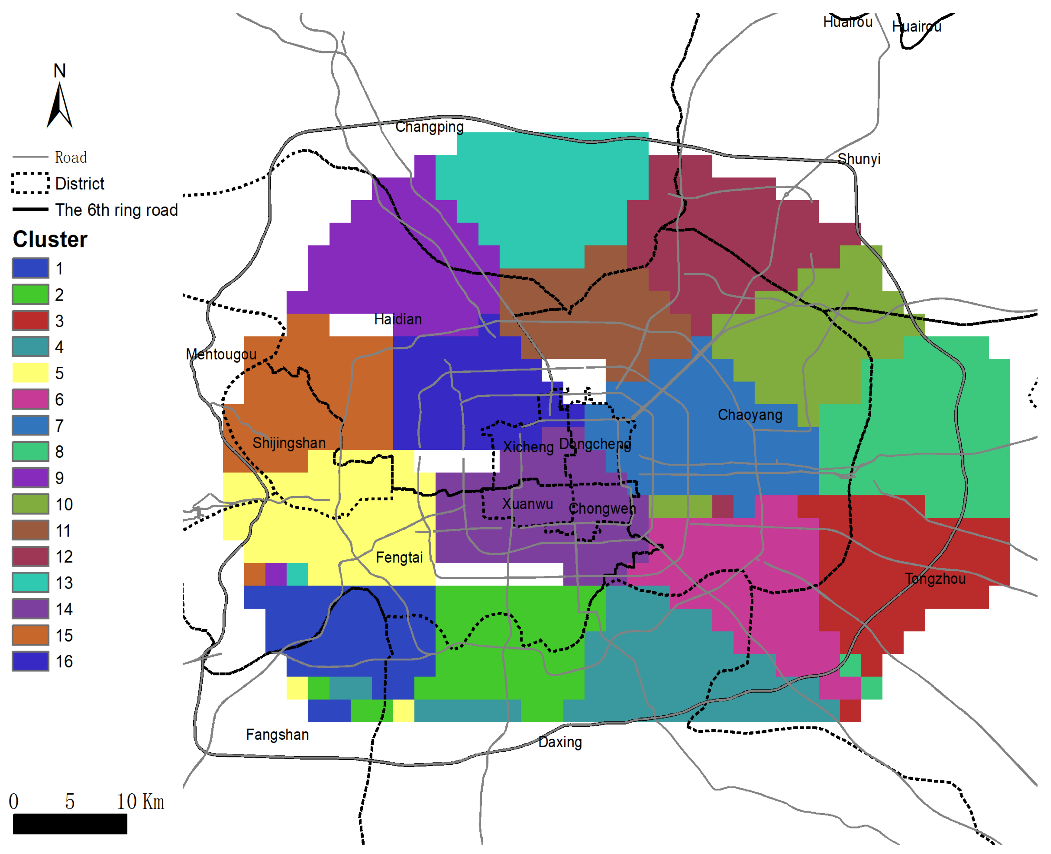
3.2. Boundaries of Housing Market and Submarkets in Beijing

Figure 3 plots the segmentation of the housing market in Beijing, generated on the set of 1000 m × 1000 m grids and colored according to the cluster membership of every grid. Hotspot analysis was applied to all grids and those “cold-spot” grids where few housing units being transacted were removed nearby. The remaining grids give a sketch of the natural boundary of the entire housing market. It is clear that second-hand housing market in Beijing is agglomerated in the area enclosed by the sixth-ring road, which is also known as a cut-off of urban-suburb and exurb area of Beijing. In addition, the housing market region is not quite symmetric according to the distance between the boundary of the market and sixth-ring road. Comparing to the south and west boundary, the distance between sixth-ring road and the north and east side of boundary of housing market is much smaller; this asymmetricity reflects that the northern and eastern parts of Beijing lead its southern and western parts in terms of economic development and completeness of infrastructures [63].
The entire housing market is divided into submarkets through constrained clustering. For robustness checking, we re-ran the algorithm 100 times under random initialization; the number of clusters returned varied from 14 to 16, and the range of each submarket was not significantly distinct based on comparing the Hausdorff distance between a submarket in one set of result with the nearest submarket in the other set of result. The small variance of clustering result with respect to random initiation shows the stability of our result. Through comparing the BIC of 100 results, we finally selected one set of submarket divisions which had 16 submarkets. The location and the range of every submarket are plotted in Figure 3. To facilitate the comparison, the range of administrative districts are sketched in Figure 3, illustrating that the range of submarkets significantly disagrees with administrative regions. This fact confirms the invalidity of directly using administrative districts as intra-urban analogue to cities in inter-urban spillover analysis.
Figure 3 also shows that spatial distribution of submarkets displays a sprawl pattern. More precisely, submarkets are clearly stratified to two layers according to their distance to the center of Beijing, marked as the Ti’an Men Square. Every layer is roughly annular-shaped; the number of submarkets lying on layers is increasing along the direction from the inner layer (closer to center) to outer layers (further away from center). This annular-sprawl pattern of submarket distribution reflects the mono-centric city structure of Beijing, as does the fact that we utilized k-means as the base clustering tool for constrained clustering, which forces every cluster to be as compact as possible.

3.3. Robustness Analysis by Policy Shock

Beijing attempted to restrict its housing market in order to squeeze the price “bubble” induced by housing speculation. Unlike indirect restrictions, such as taking the property tax [64], since the third quarter of 2013, the local government of Beijing initiated a series of intervention policies to control the market demand, including lifting up interest rate and down-payment rate of mortgage, quota restricting and freezing transactions that involved non-local buyers. The entire housing market in Beijing cooled down sharply since then, and entered a depression period until late 2016 when the intervention was relaxed. Therefore, there exists a major policy change during our data collection period. The shocks induced by policy changes can be formulated either as one-time shocks such that they do not affect distributional patterns of submarket and the spillover transitions between them, or as permanent effects on spillover transitions in terms of altering the submarkets’ structures and/or the transition probability matrix.
To distinguish the one-time and permanent shocks, we re-ran constrained clustering within two separated time intervals, which were (1) before 2013 Q3 and (2) after 2013 Q3. The structural change test was conducted toward the range and location of every submarket and the transition probabilities among submarkets. The null hypothesis was always that over the two periods, there would be no structural changes, for which we considered two sets of hypothesis tests:
H 0 1 : d H ( S i , S i * l ) = 0 H 0 2 : p i , j p i * , j * l = 0 .
H 0 1 is tested on the basis of empirical Hausdorff distance (16) (see the method section) between a submarket S i generated from the assumption that there were no structural changes during the entire data collection period and the submarket S i * l nearest to S i generated before ( l = 1 ) and after ( l = 2 ) the time, 2013 Q3, when intervention policy was initiated. Thus, test of H 0 1 examines whether there is location-based and/or ranging changes for submarkets.
In contrast, the test of H 0 2 examines changes of transition probability, where p i , j denotes the transition probability calculated under the assumption that no structural changes happened during the entire period, while p i * , j * l measures the transition probability between submarkets nearest to i and j respectively before 2013 Q3 when l = 1 and after 2013 Q3 when l = 2 . H 0 2 is implementable through Pearson’s χ 2 test, which can be conducted either separably for every pair ( i , j ) or in a bulk way for the sum of square difference of all ( i , j ) s. The bulk test is more informative for the overall impact of policy change, while the separate test is better at detecting its impact to specific submarkets. In this study, we first applied the bulk test for both cases of l = 1 and l = 2 . Failure to pass the bulk test indicates the occurrence of a transition probability change for some pairs of submarkets; thus, a separate test was carried out and the set of pairs that failed to pass it are reported.
Table 2 reports the Hausdorff distance tests for all 16 submarkets before and after 2013 Q3. It is apparent that at the 5 % credential level, almost all submarkets have no significant changes in their locations and ranges before and after the conduction of intervention policy. Thus, the policy does not affect the market structure of Beijing. The only exception is submarket 13; it seems to be relocated after 2013 Q3. The detailed reason of the movement of submarket 13 is interesting, but it is beyond the scope of this study; we leave it for future studies.
Table 3 reports the results of Pearson’s χ 2 test conducted in a bulk way. The transition matrix has no structural difference between the entire data collection period and the period after policy change. However, interventions make difference for period before 2013 Q3, which is reflected by the null hypothesis H 0 2 failing to hold before 2013 Q3.
To better detect where policy changes matter, separated Pearson’s χ 2 tests were conducted; Table 4 collects all pairs of submarkets that failed to pass the test on a 5 % credential level, in which the results have been sorted, along with their p-values, in an ascending way:
As shown in Table 4, there are 30 out of 256 (= 16 × 16 ) different pairs of submarket combinations whose transition probabilities did not pass the χ 2 test. Thus, the main portion of submarket pairs were still quite stable facing intervention policies, which implies an overall robustness of the spillover mechanism of the housing market in Beijing. Among those pairs whose transition probabilities were changing as policy changed, Table 4 indicates that all of them are ended up with one of the three submarkets, 1, 10, or 11. In fact, for all the three regions, both of transit-in/-out probabilities from/to all the other regions are much smaller in relation to the other regions; the significance before and after the policy change just reflects the sensitivity of the small number. Hence, we can conclude the intervention policy did not entail significant change to the spillover mechanism; it can be considered persistent over the entire data collection period during 2011–2017.

3.4. Factors Affecting Spillover

In this section, we describe regression analysis performed to identify the factors that have strongest connection to the intensity of spillover transitions. Among all factors, we were mainly concerned with the impacts of distance, price difference, area difference, and location among submarkets on the transition probabilities, because a preliminary analysis showed that among all alternative covariates, these five classes of variable were sufficient to account for above 90 % of the total variation of transition probabilities. Formally, we estimate regression equation of the following form:
T i , j = β 0 + β 1 · d i s t a n c e i , j + β 2 · p r i c e _ d i f i , j + β 3 · l a t i + β 4 · l a t j + β 5 · l o n i + β 6 · l o n j + ε i , j ,
and for a robustness check, we also considered the alternative regression equation:
T i , j = β 0 + β 1 · d i s t a n c e i , j + β 2 · p r i c e _ d i f i , j + β 3 · l a t _ d i f i , j + β 4 · l o n _ d i f i , j + ε i , j
where p i , j are the transition probabilities between submarket i and j; d i s t a n c e i , j is the center distance between two submarkets (i.e., the euclidean distance between the centers of two submarkets); and p r i c e _ d i f i j is the mean difference of price (i.e., the difference between the within-cluster means of two submarkets). ε i , j is the residual. (20) differs from (21) in the sense that whether the relative location between transit-in and transit-out submarkets or the exact location of them is involved. In (20), exact location is included through the latitudes and longitudes of centers of transit-out and transit-in submarkets, which provide more information.
In the preliminary analysis, we tried both (20) and (21). The final result reported in Table 5 was selected as the one generated from the equation that had the greatest explanatory power for the data (measured by the a d j . R 2 statistics). In addition to taking the entries of the transition matrix T as dependent variables, we also considered the regression based on using the net transit-out probability; namely, entries of T T , as the dependent variable. The regression for the net transit-out probability can help detect the source of the spillover effect; the result reported is also based on the combination that generates the greatest a d j . R 2 .
Table 5 shows that the regression model (20) has better explanatory power for the full transition probability T , while (21) fits better to the net transit-out probability T T . This fact implies that the exact locations of both the transit-out and transit-in submarkets matter to the full transit probability, while only the relative position between the two submarkets matters to the net transit probability. Such a difference should reflect some deep-level mechanism behind the intra-urban housing market spillover, which is a bit beyond the scope of the current study, so we left it for future works.
Table 5 also reveals that no matter what type of transit probability we consider, the distance between two submarkets is either irrelevant or positively contribute to the probability. This fact implies that in intra-urban setting, geographic neighborhood is no longer a major mechanism through which spillover can happen, so housing market spillover is not of the “ripple” form, which is quite different from the findings from inter-urban spillover [20,21]. On the other hand, the difference of price between submarkets turns out to have significant positive impact on transition probability. This finding agrees with the argument that the existence of price gap and price-depressed regions is sufficient to intrigue housing market spillover, even if there are geographic gaps between transit-in and transit-out regions. Unlike “ripple” effect, spillover induced purely by price gap allows geographic discontinuity; thus, it is classified as a migration effect [65] in order to be distinguished from the “ripple” effect, which requires geographic continuity.
In inter-urban spillover studies, the migration effect is extremely weak, but it is dominant in our current study. We believe the difference in strength of the migration effect to be by and large attributable to the distinct transition mechanisms between inter-urban and intra-urban spillovers. In the intra-urban case, relocation cost is usually low in contrast to the cost of housing; this is true especially for a city like Beijing where the ratio between income and housing price can even exceed 100+. Thus, comparing to the limited transaction cost induced by relocation, moving into a price-depressed region is much more profitable and should be able to intrigue huge and immediate move-in flows and drive up local housing prices. In contrast, at the inter-urban scale, relocation costs are always extraordinarily high compared to price differences in two distant cities; the high transaction cost restricts long-distance relocation, and thus reduces the strength of the migration effect; spillovers are only possible to exist between neighborhoods, which leads to the widely documented “ripple” effect [20,21]. The finding from Table 5 supports that argument; it also highlights the theoretical necessity to distinguish intra-urban spillover from inter-urban spillover.
From the perspective of spatial variation, an interesting finding from Table 5 is that probability of spillover transit-in, which is just the negative transit out probability, is decreased along with the direction from southeast to northwest in Beijing. This finding coincides with a fact that the northwest part of Beijing is much more well-developed in terms of the concentration of high-tech industry, educational resources, and the absolute value of housing prices (high); the increasing strength of spillover transit-in is then a reflection of the equalization effect of housing market spillover, as widely discussed in the literature [7].

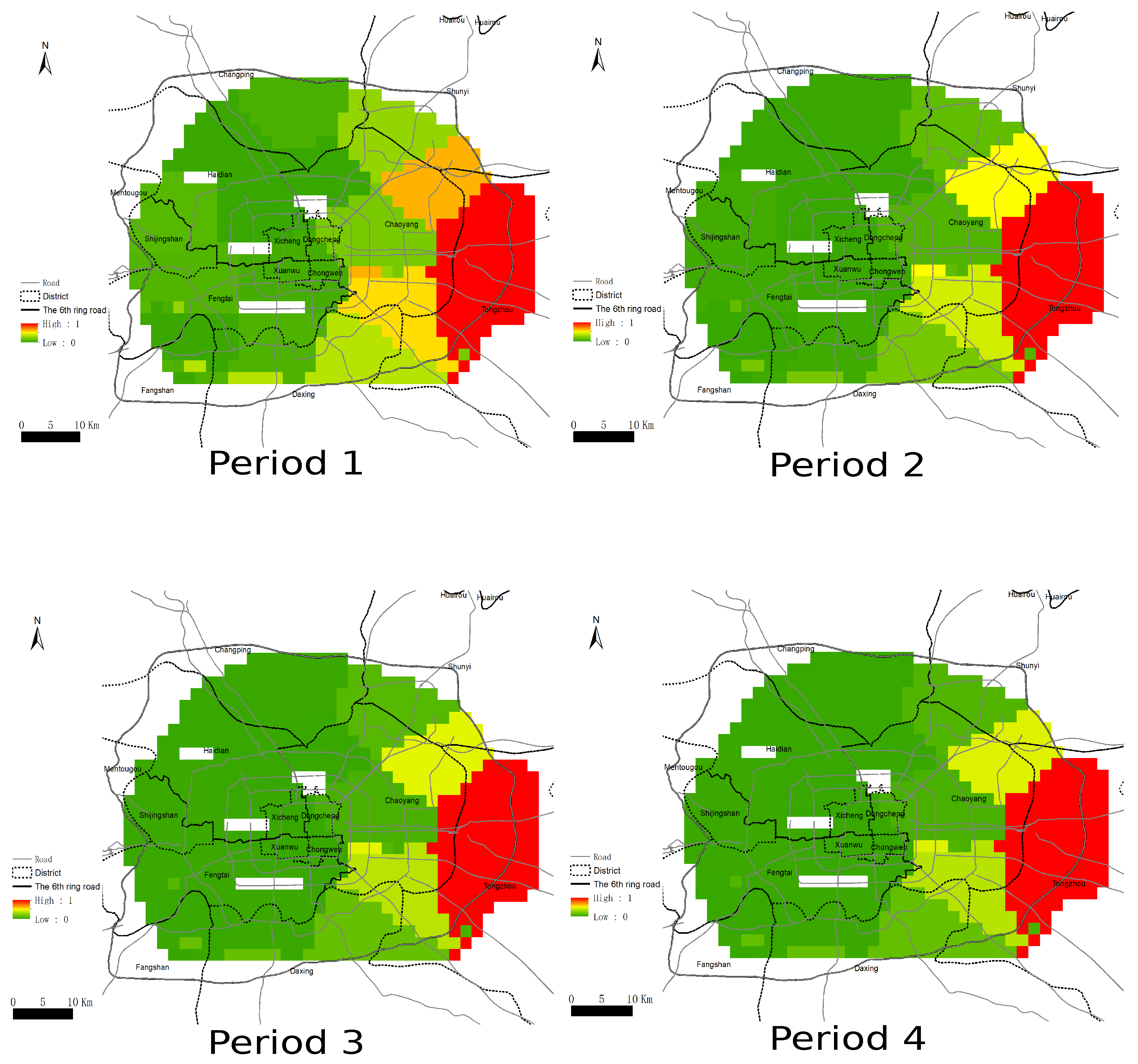
3.5. Transition Intensity of Multi-Period Spillovers

In this section, we study the spatio-temporal variation pattern of spillover intensity in Beijing through applying the methodology introduced in the Methods section.
By letting t vary, we can evaluate the spatio-temporal trend of CI t , which sketches the relative strength of driving force distributed among submarkets by time t. It turns out the variation of CI t becomes stable. Since t = 4 (measured by time difference CI t being less than a threshold value, say 0.01 ), we plot the spatial distribution of CI t up to time 4 in Figure 4.
As shown in Figure 4, driving forces of the housing market in Beijing are inclined to spread from its northern and western parts to the south and to the east, this dynamic pattern agrees with the regression result shown in previous section. On the other hand, two submarkets in east-most area of the entire study area have the greatest long-term transit-in intensity, and both of these two submarkets are located within the Tongzhou district of Beijing and next to the western boundary of Tongzhou district and the city core of Beijing. It is remarkable to notice that these two regions cover exactly Tongzhou, the new city which is planned to absorb most of administrative departments, schools, and medical facilities that were originally located in the core of Beijing. This finding reveals the large influence of urban planning policy on mechanisms of housing market spillover in China, and it also reflects the consistency between the trends of housing market spillover and reallocation of valuable public resources.

4. Discussion

Based on the findings in the previous sections, some useful policy suggestions can be derived. First, the ultimate direction of spillover is largely affected by the official urban planning proposal (Figure 4). This fact implies that on one hand, the local government can significantly manipulate the way by which spillover happens, but on the other hand, the government’s behavior can induce inequality in housing prices for different regions. The case of Beijing shows that the submarkets close to Tongzhou (covered by the red color in Figure 4) benefit significantly from the urban planning in terms of the appreciation of housing price; the price gap between Tongzhou and the old core region, exemplified by the submarket covering the Zhongguan Village (Cluster 1 in Figure 3), almost vanished according to Figure 3. In contrast, the submarkets (e.g., the Clusters 1 and 2 in Figure 3) in the southwest part of Beijing did not get much from the price spillover, and the price gap between there and the Tongzhou is even enlarged in Figure 2. Based on its influence on spillover and price distribution, and the fact that the relative change of housing prices is closely related to the re-distribution of family wealth and social welfare, we believe the local government should be cautious before issuing any planning proposal. Second, the intra-urban spillover turned out to be discontinuous geographically and price-gap driven (Table 5) in Beijing. This observation implies that speculation might be the main force driving the housing price dynamics, which is not healthy for housing market development and urban growth in the long run. Therefore, stabilizing the housing price variation and controlling the speculative transaction should be a main targets of local housing policy in Beijing in the future. Finally, the regular marketization intervention policies, such as increasing the down-payment rate and assigning purchase quota to home-buyers, turned out to be ineffective at controlling the long-term spillover trend and housing price dynamics, which recalls policy innovation. More non-marketization tools can be taken into account, such as increasing the supply of public housing.

5. Conclusions

This paper analyzed the intra-urban spillover of Beijing through a constrained-clustering-based Markov chain model. The empirical result shows that first, the intra-urban spillover of housing price occurs quite differently compared to the widely studied inter-urban spillover. In particular, the widely observed “ripple-form” spillover in inter-urban setting is no longer dominant in the intra-urban setting. In contrast, intra-urban spillover can be discontinuous in the geographic sense, and is mainly driven by price gap and speculative demand. Second, the urban planning policies can entail significant impacts on housing market spillover, while the pure intervention on housing prices based on marketization methods seems not to be quite influential. This finding implies the effectiveness of policy varies from case to case; the determinants have not yet attracted enough attention and deserve further investigation.
Other than the empirical findings, this study also has a methodological contribution for the existing literature. The constrained clustering technique not only applies to intra-urban housing market spillover, but is very helpful to a wide range of spatio-temporal topics where the nodes among which a spatio-temporal effect takes place are not clearly defined beforehand.
Some limitations and possible extensions are identified as below. First of all, only the direction and intensity of each spillover were included in the constrained clustering framework, and the scale of spillover was not referred to. A more comprehensive study is needed in the follow-up research. Time series models such as the vector autoregressive model (VAR) are powerful for modeling the transition scale, and how to embed it into the constrained clustering is a promising direction for the future research. In addition, the covariate is not yet included for determining the transition probability, so extending the current framework to embrace the covariate is important for better understanding the mechanism of the spillover transition.

Author Contributions

Daijun Zhang and Xinyue Ye conceived the study. Daijun Zhang, Xiaoqi Zhang, and Yanqiao Zheng designed the methodology and implemented the main computation. Shengwen Li and Qiwen Dai provided the visualization of the data and analytic results. Daijun Zhang and Xinyue Ye wrote the manuscript. Xiaoqi Zhang, Xinyue Ye, and Shengwen Li advised the interpretation of the results. All authors have read and agreed to the published version of the manuscript.

Funding

This research was funded by the National Natural Science Foundation of China under grant number 11801503 and 41801378. The APC was funded by the National Natural Science Foundation of China under grant number 11801503.

Conflicts of Interest

The authors declare no conflict of interest.

Appendix A. Data Summary

Table A1. Summary of major variables in the collected housing sales data.
Beijing
VariableMeaningMinMaxMeanStd.
Construction
area (m2)Construction area (m2)10.514087.3810.1
ageThe age (years) of the apartment
unit (2017 minus the year built)
05912.236.98
SouthWhether the orientation direction
includes south (south, southeast,
southwest, etc., 1 = yes, 0 = no)
010.80.4
lobby numThe number of lobby rooms081.70.79
room numThe number of bedrooms192.791.19
floorThe floor level that
an apartment is on
15743.9
Public Transport
dist subwayDistance (km) to
the nearest metro station
0.131.51.142.94
dist busDistance (km) to
the nearest bus station
0.118.170.413.06
num bus routesNumber of bus routes offered
by the nearest bus station
within 1 km
031284.4258.84
Neighborhood
dist schoolDistance (km) to nearest
primary and middle school
0.118.540.692.83
dist mallDistance (km)
to nearest mall
0.1131.51.153.13
dist hospitalDistance (km)
to the nearest hospital
0.1629.672.440.29

References

  1. Ashworth, J.; Parker, S.C. Modelling regional house prices in the UK. Scott. J. Political Econ. 1997, 44, 225–246. [Google Scholar] [CrossRef]
  2. Peterson, W.; Holly, S.; Gaudoin, P.; Britain, G. Further Work on an Economic Model of the Demand and Need for Social Housing; Stationery Office: London, UK, 2002. [Google Scholar]
  3. Cook, S. The convergence of regional house prices in the UK. Urban Stud. 2003, 40, 2285–2294. [Google Scholar] [CrossRef]
  4. Du, Q.; Wu, C.; Ye, X.; Ren, F.; Lin, Y. Evaluating the Effects of Landscape on Housing Prices in Urban China. Tijdschriftvoor Economische En Sociale Geografie 2018, 109, 525–541. [Google Scholar] [CrossRef]
  5. Holmes, M.J.; Grimes, A. Is there long-run convergence among regional house prices in the uk? Urban Stud. 2008, 45, 1531–1544. [Google Scholar] [CrossRef] [Green Version]
  6. Barros, C.; Gil-Alana, L.; Payne, J. Tests of convergence and long memory behavior in us housing prices by state. J. Hous. Res. 2013, 23, 73–87. [Google Scholar]
  7. Chow, W.W.; Fung, M.K.; Cheng, A. Convergence and spillover of house prices in chinese cities. Appl. Econ. 2016, 48, 4922–4941. [Google Scholar] [CrossRef]
  8. DeFusco, A.; Ding, W.; Ferreira, F.; Gyourko, J. The role of price spillovers in the American housing boom. J. Urban Econ. 2018, 108, 72–84. [Google Scholar] [CrossRef]
  9. Cohen, J.P.; Zabel, J. Local house price diffusion. Real Estate Econ. 2018. early view. [Google Scholar] [CrossRef]
  10. Alper, O.; Ertugrul, H.; Coskun, Y. A dynamic model for housing price spillovers with an evidence from the US and the UK markets. J. Cap. Mark. Stud. 2018, 2, 70–81. [Google Scholar]
  11. Pijnenburg, K. The spatial dimension of US house prices. Urban Stud. 2017, 54, 466–481. [Google Scholar] [CrossRef]
  12. Won, J.; Lee, J.S. Investigating How the Rents of Small Urban Houses are Determined: Using Spatial Hedonic Modeling for Urban Residential Housing in Seoul. Sustainability 2018, 10, 31. [Google Scholar] [CrossRef] [Green Version]
  13. Rangan, G.; Sun, X. Housing market spillovers in South Africa: Evidence from an estimated small open economy DSGE model. Empir. Econ. 2018, 58, 1–24. [Google Scholar]
  14. Cakan, E.; Demirer, R.; Gupta, R.; Uwilingiye, J. Economic Policy Uncertainty and Herding Behavior: Evidence from the South African Housing Market. Adv. Decis. Sci. 2019, 23, 1–25. [Google Scholar]
  15. Li, S.; Ye, X.; Lee, J.; Gong, J.; Qin, C. Spatiotemporal Analysis of Housing Prices in China: A Big Data Perspective. Appl. Spat. Anal. Policy 2017, 10, 421–433. [Google Scholar] [CrossRef]
  16. Meen, G. Regional house prices and the ripple effect: A new interpretation. Hous. Stud. 1999, 14, 733–753. [Google Scholar] [CrossRef]
  17. Murphy, A.; Muellbauer, J. Explaining Regional House Prices in the UK; Department of Economics, University College Dublin: Dublin, Ireland, 1994. [Google Scholar]
  18. Tajani, F.; Morano, P.; Saez-Perez, M.P.; Di-Liddo, F.; Locurcio, M. Multivariate Dynamic Analysis and Forecasting Models of Future Property Bubbles: Empirical Applications to the Housing Markets of Spanish Metropolitan Cities. Sustainability 2019, 11, 3575. [Google Scholar] [CrossRef] [Green Version]
  19. Stein, J.C. Prices and trading volume in the housing market: A model with down-payment effects. Q. J. Econ. 1995, 110, 379–406. [Google Scholar] [CrossRef]
  20. Gordon, I. Housing and labour market constraints on migration across the north-south divide. Hous. Natl. Econ. 1990, 75–89. [Google Scholar]
  21. Holmans, A.E. House Prices: Changes through Time at National and Sub-National Level; Department of the Environment London: London, UK, 1990. [Google Scholar]
  22. Wu, C.; Ye, X.; Ren, F.; Wan, Y.; Ning, P.; Du, Q. Spatial and Social Media Data Analytics of Housing Prices in Shenzhen, China. PLoS ONE 2016, 11, e0164553. [Google Scholar] [CrossRef]
  23. Holmans, A. What has happened to the north-south divide in house prices and the housing market. Hous. Financ. Rev. 1995, 96, 25–31. [Google Scholar]
  24. Wu, C.; Ye, X.; Du, Q.; Luo, P. Spatial Effects of Accessibility to Parks on Housing Prices in Shenzhen, China. Habitat Int. 2017, 63, 45–54. [Google Scholar] [CrossRef]
  25. Hui, E.; Wang, Z. Market sentiment in private housing market. Habitat Int. 2014, 44, 375–385. [Google Scholar] [CrossRef]
  26. Munro, M.; Maclennan, D. Intra-urban changes in housing prices: Glasgow 1972–1983. Hous. Stud. 1987, 2, 65–81. [Google Scholar] [CrossRef]
  27. Fadiga, M.L.; Wang, Y. A multivariate unobserved component analysis of us housing market. J. Econ. Financ. 2009, 33, 13–26. [Google Scholar] [CrossRef]
  28. Zhang, M.; Meng, X.; Wang, L.; Xu, T. Transit development shaping urbanization: Evidence from the housing market in beijing. Habitat Int. 2014, 44, 545–554. [Google Scholar] [CrossRef]
  29. Zhang, S.; Guldmann, J.M. Accessibility, diversity, environmental quality and the dynamics of intra-urban population and employment location. Growth Chang. 2010, 41, 85–114. [Google Scholar] [CrossRef]
  30. Kirby, D.K.; LeSage, J.P. Changes in commuting to work times over the 1990 to 2000 period. Reg. Sci. Urban Econ. 2009, 39, 460–471. [Google Scholar] [CrossRef]
  31. Jones, C.; Leishman, C.; Watkins, C. Intra-urban migration and housing submarkets: Theory and evidence. Hous. Stud. 2004, 19, 269–283. [Google Scholar] [CrossRef]
  32. Schelling, T.C. Dynamic models of segregation. J. Math. Sociol. 1971, 1, 143–186. [Google Scholar] [CrossRef]
  33. Cui, C.; Geertman, S.; Hooimeijer, P. The intra-urban distribution of skilled migrants: Case studies of shanghai and nanjing. Habitat Int. 2014, 44, 1–10. [Google Scholar] [CrossRef]
  34. Zheng, S.; Peiser, R.B.; Zhang, W. The rise of external economies in beijing: Evidence from intra-urban wage variation. Reg. Sci. Urban Econ. 2009, 39, 449–459. [Google Scholar] [CrossRef]
  35. Partridge, M.D.; Rickman, D.S.; Ali, K.; Olfert, M.R. Agglomeration spillovers and wage and housing cost gradients across the urban hierarchy. J. Int. Econ. 2009, 78, 126–140. [Google Scholar] [CrossRef] [Green Version]
  36. Njoh, A.J. Interorganisational relations and effectiveness in a developing housing policy field. Habitat Int. 1996, 20, 253–264. [Google Scholar] [CrossRef]
  37. Li, Z.; Li, X.; Wang, L. Speculative urbanism and the making of university towns in china: A case of guangzhou university town. Habitat Int. 2014, 44, 422–431. [Google Scholar] [CrossRef]
  38. Krupka, D.J.; Noonan, D.S. Empowerment zones, neighborhood change and owner-occupied housing. Reg. Sci. Urban Econ. 2009, 39, 386–396. [Google Scholar] [CrossRef] [Green Version]
  39. Clayton, J.; Ling, D.; Naranjo, A. Commercial real estate valuation: Fundamentals versus investor sentiment. J. Real Estate Financ. Econ. 2009, 38, 5–37. [Google Scholar] [CrossRef]
  40. Zhou, J.; Anderson, R.I. An empirical investigation of herding behavior in the us reit market. J. Real Estate Financ. Econ. 2013, 47, 83–108. [Google Scholar] [CrossRef]
  41. Valentini, P.; Ippoliti, L.; Fontanella, L. Modeling us housing prices by spatial dynamic structural equation models. Ann. Appl. Stat. 2013, 7, 763–798. [Google Scholar] [CrossRef]
  42. Tsai, I.C. Spillover effect between the regional and the national housing markets in the UK. Reg. Stud. 2015, 49, 1957–1976. [Google Scholar] [CrossRef]
  43. Harding, J.P.; Rosenblatt, E.; Yao, V. The contagion effect of foreclosed properties. J. Urban Econ. 2009, 66, 164–178. [Google Scholar] [CrossRef]
  44. Daneshvary, N.; Clauretie, T.; Kader, A. Short-term own-price and spillover effects of distressed residential properties: The case of a housing crash. J. Real Estate Res. 2011, 33, 179–207. [Google Scholar]
  45. Leonard, T.; Murdoch, J. The neighborhood effects of foreclosure. J. Geogr. Syst. 2009, 11, 317. [Google Scholar] [CrossRef] [Green Version]
  46. Rogers, W. Declining foreclosure neighborhood effects over time. Hous. Policy Debate 2010, 20, 687–706. [Google Scholar] [CrossRef]
  47. Ihlanfeldt, K.; Mayock, T. The impact of REO sales on neighborhoods and their residents. J. Real Estate Financ. Econ. 2016, 53, 282–324. [Google Scholar] [CrossRef]
  48. Del Giudice, V.; De Paola, P.; Forte, F.; Manganelli, B. Real Estate Appraisals with Bayesian Approach and Markov Chain Hybrid Monte Carlo Method: An Application to a Central Urban Area of Naples. Sustainability 2017, 9, 2138. [Google Scholar] [CrossRef] [Green Version]
  49. Wu, C.; Sharma, R. Housing submarket classification: The role of spatial contiguity. Appl. Geogr. 2012, 32, 746–756. [Google Scholar] [CrossRef]
  50. Wagstaff, K.; Cardie, C.; Rogers, S.; Schrödl, S. Constrained k-means clustering with background knowledge. Icml 2001, 1, 577–584. [Google Scholar]
  51. Basu, S.; Banerjee, A.; Mooney, R.J. Active semi-supervision for pairwise constrained clustering. In Proceedings of the 2004 SIAM International Conference on Data Mining, Lake Buena Vista, FL, USA, 22–24 April 2004; pp. 333–344. [Google Scholar]
  52. Diaz-Valenzuela, I.; Loia, V.; Martin-Bautista, M.J.; Senatore, S.; Vila, M.A. Automatic constraints generation for semisupervised clustering: Experiences with documents classification. Soft Comput. 2016, 20, 2329–2339. [Google Scholar] [CrossRef]
  53. Bonhomme, S.; Manresa, E. Grouped patterns of heterogeneity in panel data. Econometrica 2015, 83, 1147–1184. [Google Scholar] [CrossRef] [Green Version]
  54. Kang, W.; Rey, S.J. Conditional and joint tests for spatial effects in discrete markov chain models of regional income distribution dynamics. Ann. Reg. Sci. 2018, 61, 73–93. [Google Scholar] [CrossRef]
  55. Wu, C.; Ye, X.; Ren, F.; Du, Q. A Modified Data-Driven Framework for Housing Market Segmentation. J. Urban Plan. Dev. 2018, 144, 04018036. [Google Scholar] [CrossRef]
  56. Getis, A.; Ord, J.K. The analysis of spatial association by use of distance statistics. Geogr. Anal. 1992, 24, 189–206. [Google Scholar] [CrossRef]
  57. Ord, J.K.; Getis, A. Local spatial autocorrelation statistics: Distributional issues and an application. Geogr. Anal. 1995, 27, 286–306. [Google Scholar] [CrossRef]
  58. Girres, J.F.; Touya, G. Quality assessment of the french openstreetmap dataset. Trans. GIS 2010, 14, 435–459. [Google Scholar] [CrossRef]
  59. Deng, M.; Li, Z.; Chen, X. Extended hausdorff distance for spatial objects in gis. Int. J. Geogr. Inf. Sci. 2007, 21, 459–475. [Google Scholar]
  60. National Bureau of Statistics. China City Statistical Yearbook; Statistics Press: Beijing, China, 2016.
  61. Zhu, R.; Wu, X. Risks and Potentials in Beijing’s Real Estate Market. Biomed. J. Sci. Tech. Res. 2018, 9, 7406–7413. [Google Scholar]
  62. Wang, F.; Gao, X. The Transitional Spatial Pattern of Housing Prices in Beijing: Factors and Implication. Int. Rev. Spat. Plan. Sustain. Dev. 2014, 2, 46–62. [Google Scholar] [CrossRef] [Green Version]
  63. Lin, G.; Zhang, A. China’s metropolises in transformation: Neoliberalizing politics, land commodification, and uneven development in beijing. Urban Geogr. 2017, 38, 643–665. [Google Scholar] [CrossRef]
  64. Tajani, F.; Morano, P.; Torre, C.; Di Liddo, F. An Analysis of the Influence of Property Tax on Housing Prices in the Apulia Region (Italy). Buildings 2017, 7, 67. [Google Scholar] [CrossRef] [Green Version]
  65. Meen, G. Spatial aggregation, spatial dependence and predictability in the uk housing market. Hous. Stud. 1996, 11, 345–372. [Google Scholar] [CrossRef]
Sample Availability: Samples of this research are available from the authors.
Figure 1. Study area and spatial distribution of samples.
Ijgi 09 00056 g001
Figure 2. Spatio-temporal distribution of samples.
Ijgi 09 00056 g002
Figure 3. Boundaries of housing (sub-)markets in Beijing.
Ijgi 09 00056 g003
Figure 4. Evolution of the distributional density of market driving force.
Ijgi 09 00056 g004
Table 1. Important socioeconomic features of Beijing.
CityCenter Location
(Lat, Lon)
GDP (billion
RMB)
Population Size
(million)
Built Area
(km2)
# County-Level
Administrative Units
# Subway Lines
Beijing39.9° N, 116.41° E280021.714191618 up to Nov. 2017
Table 2. Hausdorff test.
Before 2013 Q3 After 2013 Q3
ClusterNearest-Distancep-Value0.05 CINearest-Distancep-Value0.05 CI
10.06110.820.0940.9860.76
20.0980.9990.50.06310.92
30.160.3450.320.0980.9990.69
40.1520.510.360.1840.9990.73
50.080.960.60.04410.88
60.10710.710.0920.9990.73
70.1210.7880.720.1380.6710.39
80.1080.2030.140.0790.9990.68
90.1260.2390.240.0990.9940.5
100.1230.0760.160.1310.9980.7
110.1120.6750.70.1130.8310.49
120.2360.0020.060.1880.3090.39
130.1730.4980.690.1750.0040.06
140.120.8330.390.1210.9390.49
150.06110.850.0990.9990.74
160.0980.8130.540.1240.5050.53
Table 3. χ 2 test (bulk).
PeriodTest-Statisticsp-Value0.05_CI
Before 2013 Q3501.5230294.321
After 2013 Q3208.790.986
Table 4. χ 2 test (separated).
#VarTest-Statisticsp-Value
1 p 6 , 11 13.0020.0003
2 p 7 , 11 12.3070.0005
3 p 1 , 10 11.8710.0006
4 p 12 , 11 11.6820.0006
5 p 3 , 11 11.5890.0007
6 p 6 , 10 11.420.0007
7 p 2 , 10 10.8490.001
8 p 7 , 10 10.8140.001
9 p 2 , 11 10.5750.001
10 p 5 , 10 10.5310.001
11 p 5 , 11 10.3840.001
12 p 12 , 10 10.3020.001
13 p 1 , 11 9.9910.002
14 p 3 , 10 9.7710.002
15 p 16 , 11 7.7220.005
16 p 4 , 11 7.3650.007
17 p 14 , 11 6.7770.009
18 p 16 , 10 6.7660.009
19 p 4 , 10 6.7460.009
20 p 14 , 10 5.9520.015
21 p 1 , 1 5.0830.024
22 p 10 , 11 5.0510.025
23 p 6 , 1 4.7080.03
24 p 2 , 1 4.6490.031
25 p 5 , 1 4.4760.034
26 p 7 , 1 4.3850.036
27 p 10 , 10 4.3410.037
28 p 12 , 1 4.180.041
29 p 11 , 11 4.0180.045
30 p 8 , 11 3.8870.049
Table 5. Regression analysis for transition probability.
Model Selected (20)TModel Selected (21) T T
distance0.0135 **distance∼0
price_dif0.0283 ***price_dif0.0566 ***
area_dif−0.0006area_dif−0.0011
out_lon0.0083diff_lon−0.0291 ***
in_lon0.0029--
out_lat−0.0187 ***diff_lat0.0054
in_lat−0.0128 ***--
Adj. R20.984Adj. R20.849
F-statistic2275 ***F-statistic287.8 ***
*: 10% significant, **: 5% significant, ***: 1% significant.

