Multi-Parameter Estimation of Average Speed in Road Networks Using Fuzzy Control

Abstract

Average speed is crucial for calculating link travel time to find the fastest path in a road network. However, readily available data sources like OpenStreetMap (OSM) often lack information about the average speed of a road. However, OSM contains other road information which enables an estimation of average speed in rural regions. In this paper, we develop a Fuzzy Framework for Speed Estimation (Fuzzy-FSE) that employs fuzzy control to estimate average speed based on the parameters road class, road slope, road surface and link length. The OSM road network and, optionally, a digital elevation model (DEM) serve as free-to-use and worldwide available input data. The Fuzzy-FSE consists of two parts: (a) a rule and knowledge base which decides on the output membership functions and (b) multiple Fuzzy Control Systems which calculate the output average speeds. The Fuzzy-FSE is applied exemplary and evaluated for the BioBío and Maule region in central Chile and for the north of New South Wales in Australia. Results demonstrate that, even using only OSM data, the Fuzzy-FSE performs better than existing methods such as fixed speed profiles. Compared to these methods, the Fuzzy-FSE improves the speed estimation between 2% to 12%. In future work, we will investigate the potential of data-driven machine learning methods to estimate average speed. The applied datasets and the source code of the Fuzzy-FSE are available via GitHub.

1. Introduction

Applications like route planning, disaster risk management or transportation depend on finding the fastest path in a road network. For the computation of the fastest path, average speed values are assigned to every edge in the road network to calculate link travel times. The link travel time is the average time a vehicle spends traveling along a network edge [1]. In studies on critical road infrastructure and accessibility, the link travel time often serves as a cost factor for the road network [2,3,4,5].

Many of these approaches use OpenStreetMap (OSM) data. The OSM project provides free worldwide road network data that are collected and maintained by volunteers worldwide. Everyone can register as an OSM user and participate. Barrington-Leigh and Millard-Ball [6] have concluded in 2017 that the OSM road network is more than 80% complete. Moreover, 40% of all countries in the worldwide OSM dataset have a fully mapped road network. Due to the open and free character of OSM, many approaches using its data raised the question of data quality which caused a number of investigations on that topic. To summarize the results, OSM can be accurate and complete and in some regions it can compete with or even be better than commercial or administrative datasets [7,8,9,10,11,12,13,14]. In some developing countries, the completeness of the road network is high at a national level [15,16].

The OSM road network data can be imported into a topological data structure for usage in routing applications. While the road network quality is satisfying for most approaches, additional attributes for its edges are needed for routing. In OSM, it is possible to include additional attributes to every road element. By this way, information on maximum speed for every road element can be added. However, most roads lack this information. 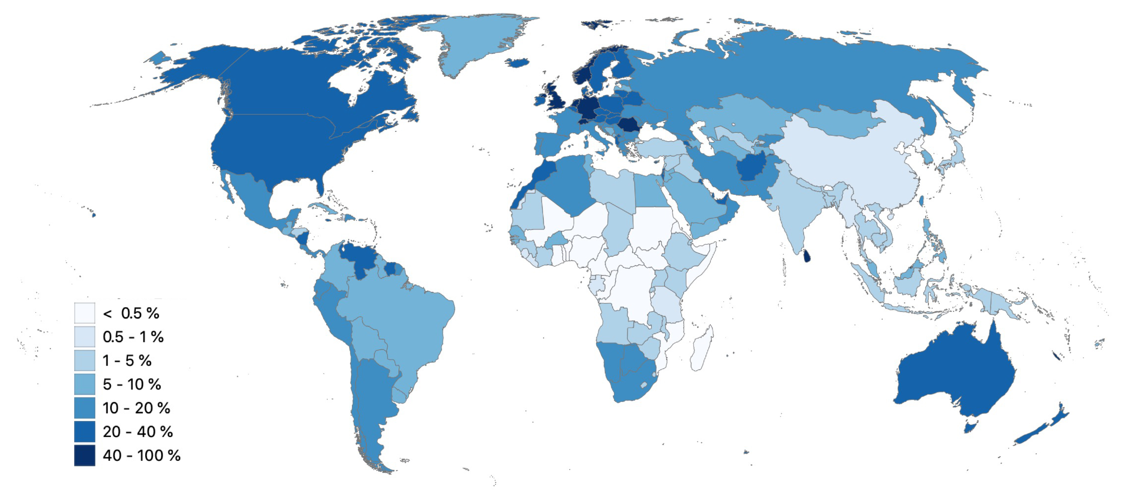Figure 1 shows the proportion of the total length of the upper level roads (as defined in

Table 1. Road classes in the OSM road network, taken from [18].

Road Class	Description
Motorway	Restricted access, major divided highway.
Trunk	Most important roads in a country’s system that are not motorways.
Primary	Major highways, linking large towns.
Secondary	Highways, not part of a major route, form a link in the national route network, often link towns.
Tertiary	Connect smaller settlements and minor streets to more major roads.
Unclassified	Minor public roads, lowest level of the network, often link villages and hamlets.

) with maximum speed information per country. Only $7.4$% of all road elements in the worldwide OSM dataset released in October 2019 have a maximum speed information. However, to compute link travel times and fastest paths, maximum speed information for every edge in the road network is crucial.

Influencing factors on average speed in urban and in rural areas differ for many reasons. While traffic, turn restrictions, one-way streets and traffic signals have a noticeable impact on average speed in the city, other factors dominate in rural areas. For example, the road quality has a considerable impact on the average speed: asphalted roads e.g., allow for a higher speed than unsealed gravel or mud roads. The road width and number of lanes also have an impact on speed, as well as the topography [17]. The slope of a road limits the driving speed, both by increasing sinuosity and by the slope itself.

Many studies and routing applications rely on fixed speed profiles for every road class defined by various input parameters. To avoid jumps at these class borders, a fuzzy control system (FCS) can be used. Such a FCS is able to fuzzify these input parameters and provides a more continuous, nonlinear output. Furthermore, it is based on expert knowledge and does not rely on reference data to learn its behavior.

This study is an extension of our previous work [18], which was published at the 5th International Conference on Geographical Information Systems Theory, Applications and Management in Heraklion, Greece. Focusing on rural road networks, we develop a Fuzzy Framework for Speed Estimation (Fuzzy-FSE) to estimate the average speed on roads in the network. The speed is derived from multiple input parameters: road hierarchy level, surface, slope and link length. The OSM road network and SRTM (Shuttle Radar Topography Mission) data serve as input data for the Fuzzy-FSE. Two different approaches are presented: the first approach relies solely on OSM data. It uses the number of support points of the vector shape of a road as an approximation for the slope (see Section 3.1). The second approach calculates road slope from an SRTM digital elevation model. The Google Directions application programming interface (GD-API) is used as reference data and as input for a baseline calculation. The Fuzzy-FSE contains multiple FCSs which are employed to obtain a continuous speed output. The FCSs are set up with the same membership functions (MF) for the input parameters slope and link length and different MF for the output parameter speed. Two exemplary case studies are performed: One in the BioBío and Maule (BM) region in Chile and the other in the north of New South Wales (NNSW) in Australia.

The main contributions of this paper are summarized as follows:

• development of a multi-parameter Fuzzy-FSE containing a combination of multiple FCS;
• a detailed analysis and discussion of the performance of the Fuzzy-FSE in comparison to an existing method;
• usage of only open source and worldwide available data (OSM, SRTM);
• transferability of the presented method to other regions;
• possibility to use the Fuzzy-FSE only with OSM data as input;
• exemplary case studies in the BioBío and Maule region in Chile and in New South Wales in Australia;
• the datasets and the implementation of the Fuzzy-FSE are published on GitHub [19].

In this paper, we first provide an overview of the related work on average speed and link travel time in OSM in Section 2.1 and introduce the concept of Fuzzy Control in Section 2.2. A detailed listing of additions and extensions compared to our previous study is given in Section 2.3. The OSM, SRTM and GD-API datasets are described in Section 3. Then, the developed Fuzzy-FSE with the FCSs is explained in Section 4. A description of both case studies (Section 5), the results (Section 6) and a detailed discussion (Section 7) are presented. Finally, a conclusion and an outlook are given in Section 8.

2. Related Work

In this section, we briefly introduce the related work on two topics. Section 2.1 and Section 2.2 are a direct quote from our previous work [18]. First, we investigate how link travel time is calculated in other approaches that rely on OSM data. Then, we introduce the concept of Fuzzy Control, its advantages and how other studies apply this concept. Finally, the major additions of this study in comparison to our previous work are presented in Section 2.3.

2.1. Link Travel Time in OSM

Many routing applications exist that compute fastest paths, and consequently link travel time, and are based on OSM data. Popular examples are the OpenRouteService [20], the Open Source Routing Machine (OSRM) [21], the OpenTripPlanner [22] and YOURS [23]. The latter three are open source applications and use the maximum speed information in OSM to calculate link travel time if available. If not, the OSM Wiki [24] contains default speed limits for some countries (24 countries worldwide), which are processed and applied by these routing applications. The applications also include other attributes like the road type and the number of lanes (if available) to derive fixed speed profiles for every road class. The algorithm for the OpenRouteService is not accessible by public. However, it seems more complex than the other routing applications as it provides additional information like the slope and type of a route. However, like many commercial routing applications such as Google Maps or Bing Maps the exact calculation is not transparent.

Few studies address the issue to derive link travel time from the OSM road network. Stanojevic et al. [1] present a methodology to calculate link travel times based on origin–destination and timestamp information generated by a taxi fleet and OSM data. They estimate travel times in urban regions with 60% lower errors than OSRM. A lot of related work concentrates on urban regions and how to improve the estimation of travel time in networks with a lot of traffic. Steiger et al. [25] include real-time traffic data into the OpenRouteService application.

As mentioned in Section 1, the important factors for routing in urban and rural areas differ considerably. In the design standards of Asian highway routes, the assigned maximum speed of a road in a rural region is directly dependent on the slope of the terrain [26]. Brabyn and Skelly [27] model access to public hospitals and calculate shortest and fastest paths. To estimate the link travel time, they consider if the road is inside or outside an urban area, the number of lanes and the sinuosity of a road. The sinuosity of a road is calculated with a sinuosity index. They categorize the roads by these factors and assign fixed velocities for every combination.

This study aims at filling some of the existent gaps in the related work. Most routing applications with OSM focus more on the city than the rural areas and only include country wide speed limits in their travel time calculation. Few studies focus on the calculation of link travel time. The ones that do rely on self-collected or commercial datasets. To our knowledge, a fuzzy control system has never been applied to estimate link travel time with different parameters.

2.2. Related Work on Fuzzy Control Systems

FCSs work on linguistic terms and partial memberships which are able to express fuzziness. An FCS takes crisp input values and fuzzifies them with the help of membership functions. In a second step, a rule base provides the basis for the inference mechanism. A defuzzification generates crisp and continuous output values.

The idea of Fuzzy Control was first introduced by [28] for a steam engine and boiler combination. Since then, Fuzzy Control has been applied successfully in various research areas: in the environmental research e.g., for flood simulation [29], in remote sensing e.g., for classification of multispectral data [30], in GIS applications [31] or in analytic chemistry [32]. Das and Winter [33] employ fuzzy logic to detect the transport mode in an urban environment.

Fuzzy Control allows for many input and many output parameters. Such parameters can be combined in an if-then rule [34]. The two greatest strengths of fuzzy control are the ability to reason with uncertainty and its utilization in complex ill-defined processes without much knowledge of their underlying dynamics [35].

2.3. Comparison to Our Previous Study

In comparison to our previous study in [18], we (a) include further input parameters (road length, road surface) for a better estimation of average speed, (b) introduce a new method to approximate road slope by using the number of support points of the vector shape of the road and thus enable the application of the Fuzzy-FSE only with OSM data and without additional data (e.g., SRTM), (c) perform a worldwide evaluation of the quality and completeness of tags (surface, lanes, width, lit) in OSM road data, (d) calculate a baseline with fixed speed profiles to compare the results against, (e) develop a new multi-parameter Fuzzy-FSE with an additional Membership Function Rule base and knowledge-base that decides which Fuzzy Control System is applied, (f) introduce multiple membership functions for speed for the different FCSs of the Fuzzy-FSE, (g) create different membership functions for the parameters slope, support points per kilometer and link length, (h) analyze the available information in OSM in the existing road network for both study regions, (i) perform additional case studies with new data in the Maule region in Chile and in New South Wales in Australia, (j) provide a detailed evaluation and discussion of the results by comparing them to the baseline and analyzing all possibilities the Fuzzy-FSE provides, (k) focus on the output average speed instead of travel time in the evaluation as it is more comparable, (l) reach new conclusions by comparing the performance of the Fuzzy-FSE in both study regions and with different modes, (m) publish the implementation of the Fuzzy-FSE on GitHub.

3. Datasets

The two datasets OSM and SRTM serve as input for the Fuzzy-FSE. The OSM dataset provides the parameters road class, road surface, link length and support points per kilometer. The road slope is calculated from SRTM data. Data from the GD-API is applied as reference data and is used as input for the speed profile. In this section, the different datasets and parameters are described.

3.1. OSM Data

OpenStreetMap road data includes a hierarchic classification of the road network that is described in Table 1. These road classes and their respective link roads (motorway_link, trunk_link, primary_link, secondary_link, tertiary_link) form the road network. Other existing road classes, such as residential and service roads or special road types like living streets, are not considered in this study.

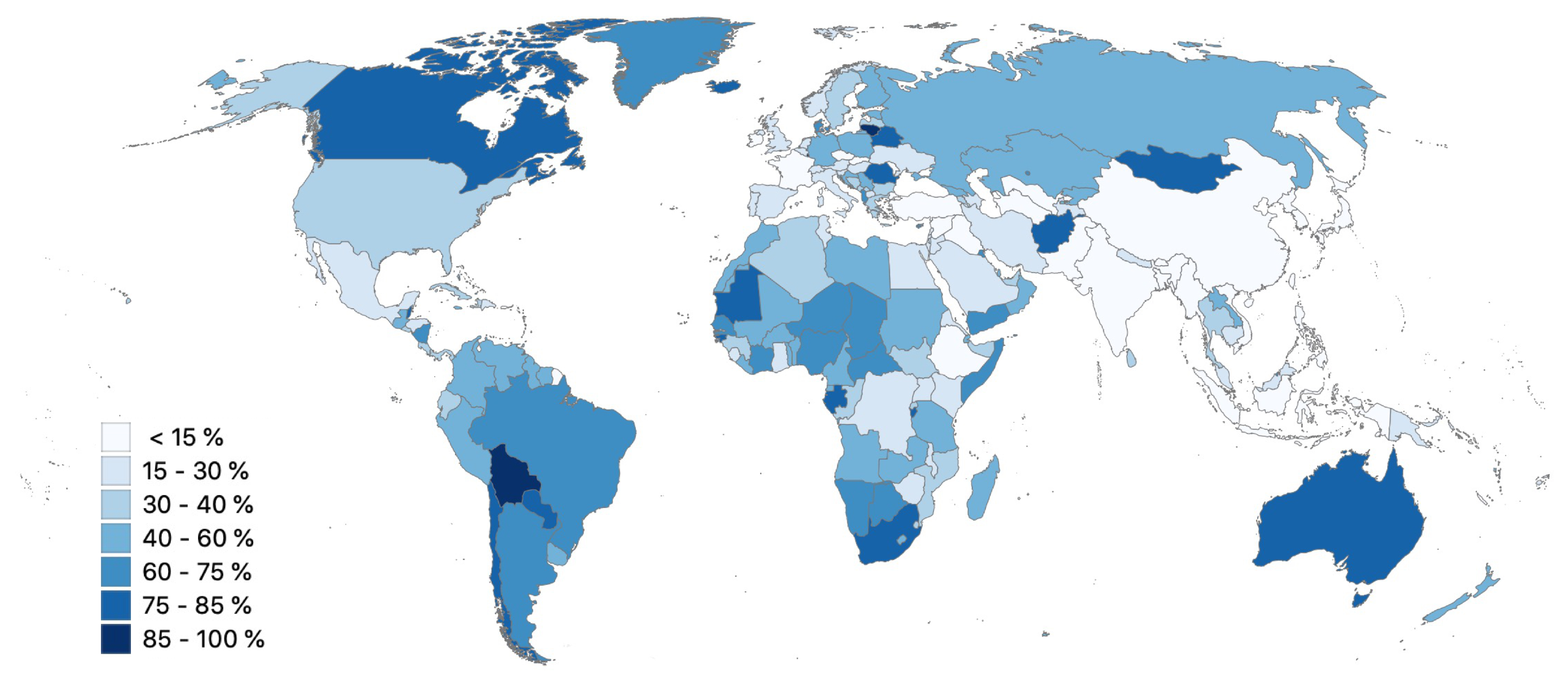
An analysis of the available attributes of roads in OSM is performed. The parameters road surface (OSM tag surface), number of lanes (OSM tag lanes), road width (OSM tag width) and illumination (OSM tag lit) are analyzed since they might be influencing factors on link travel time in rural road networks. Road surface is the most prominent of all parameters: 40% of the total length of all roads have a surface information. The distribution of the tag surface per country is shown in Figure 2. Information on the number of lanes is present in 15%, illumination in $2.2$% and road width in $0.7$% of the total length of all roads.

We include only the most frequent tag surface as an input parameter in our Fuzzy-FSE. It contains different values: general information such as paved or unpaved, and detailed description of the surface (e.g., asphalt, concrete, gravel). Most roads only feature general information; few have exact surface descriptions. For this study, the surface values are classified according to the two main groups: paved and unpaved [24].

The link length serves as an additional input parameter for the Fuzzy-FSE. The road network is represented as a graph with nodes and links. All links have a start node and an end node, but no nodes in between. In this graph, every intersection and every change of parameter in the road network represents a node. Thus, links in a sparse network are longer than in a dense network with many intersections. If there are many intersections on a road and therefore shorter links in the graph, average speed decreases.

The number of support points per kilometer is used as an approximation for slope as it can be calculated from the shape of the road in OSM. The curvier a road is, the more support points are needed to form the road and the more the average speed decreases. In OSM, the distribution of support points per road segment is not uniform. Some mappers create curves with more support points and other mappers model similar curves with much less support points. In our study, to obtain a uniform number of support points, the vector data of the road is simplified using the Douglas–Peucker algorithm [36] with a tolerance of one meter. This algorithm is applied to simplify the number of support points of the road network without an effect on the accuracy of the network in this study. Note that the overall accuracy of the OSM road network is worse than one meter. Finally, the number of support points per kilometer is calculated.

3.2. SRTM Data

The Shuttle Radar Topography Mission was a joint mission by National Imagery and Mapping Agency and the National Aeronautics and Space Administration (NASA) to collect an open source global elevation dataset. We use the SRTM void-filled, 1 arc-second global data [37] with a resolution of approximately 30 $\mathrm{m}$.

Due to this resolution, it has to be taken into account that one pixel of the SRTM raster may be the average of the road itself as well as possible hills beside that road. Therefore, we consider the slope of the surrounding terrain, which is, in most cases, higher than the actual road slope. With this in mind, we refer to the results as road slope in the following.

To calculate road slope, a slope percentage raster is created from the original DEM by applying the Horn algorithm [38]. Then, the OSM road network is overlaid with the slope raster. Every road segment intersects multiple pixels of the slope raster. The average of all intersecting pixels is assigned as road slope value to the road segment. In [18], we introduced a second approach to calculate road slope. However, the results in [18] show that the method described above better fits the problem which is why we dismiss the other approach in this study.

3.3. Google Directions API Data

The Google Directions API (GD-API) is a service that calculates routing directions and travel times between locations. The GD-API data include the distance in meters, the travel time in seconds at a given time and the coordinates of the points on a road closest to the input point coordinates. The speed values are calculated using the travel time and distance output.

The GD-API relies on Google Maps and its underlying road and traffic data. The quality of Google Maps data are difficult to assess, especially in developing countries. During our studies, both roads that exist in OSM and are non-existent in Google Maps and vice versa have been detected. In [7], the accuracy of Bing Maps, OSM data and Google Maps data in Ireland is compared and the results support our observations. The authors find that, although some areas are better served by one data source than by the others, no single data source proves to have better overall coverage. As for the speed and traffic data, there are no data available to evaluate the quality of Google Maps. We employ GD-API speed values as reference data while keeping in mind that this might, in some cases, be untrue.

Therefore, obstacles arise when comparing the output of the Fuzzy-FSE to the GD-API output. Both the Google data and the OSM data may contain errors. As the GD-API always takes the shortest path, it may take a different path between the two input coordinates than the road from which we want to compare the velocity. In addition, the travel time output of the GD-API is whole seconds. Therefore, the calculated speed of short road segments with a travel time of only few seconds may be less accurate due to rounding. An exemplary output from the GD-API of 4 $\mathrm{s}$ for a 100 $\mathrm{m}$ road segment can signify a speed of per-mode=symbol 81 $\mathrm{k}$$\mathrm{m}$/$\mathrm{h}$ (for $4.4$ $\mathrm{s}$) or per-mode=symbol 102 $\mathrm{k}$$\mathrm{m}$/$\mathrm{h}$ (for $3.5$ $\mathrm{s}$).

For this study, four types of possible errors or large inaccuracies are captured automatically and are excluded of the comparison:

• the distance between either the start or the end points on the road in OSM and in Google is larger than 50 $\mathrm{m}$;
• the lengths of the road in OSM and in Google differ in more than 20%;
• the road is shorter than 200 $\mathrm{m}$;
• the request to the GD-API returns an error or an empty result set.

To evaluate the performance of the Fuzzy-FSE, we compare it to a fixed speed profile. The speed profile assigns different speed values for each road class. Within a road class, all roads obtain the same speed value. For this study, the speed profile is derived from the average speed of the GD-API for every road class.

4. Methods

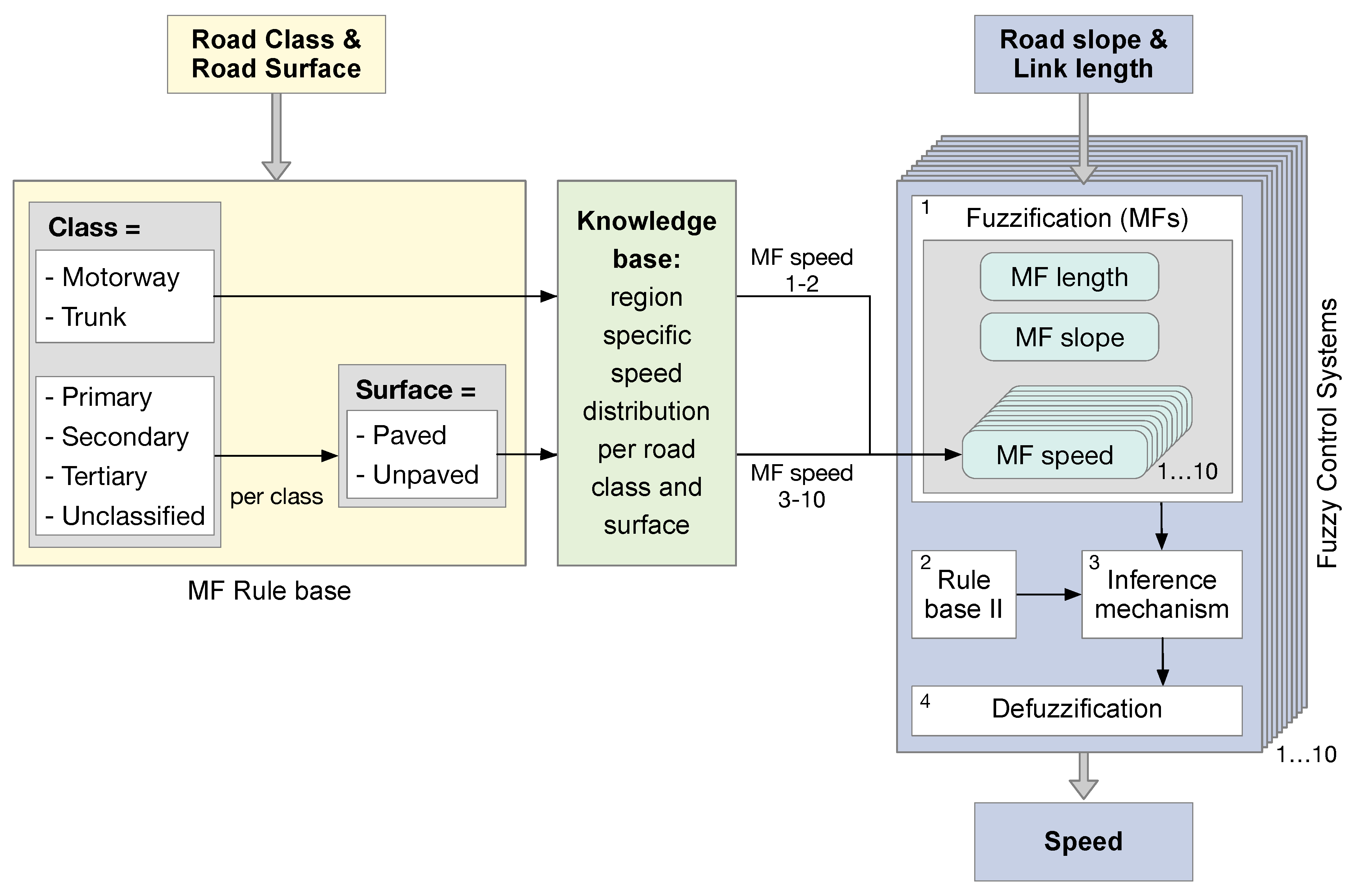
This section presents the architecture of the Fuzzy-FSE (see Figure 3). It consists of two parts: The first part is the membership function (MF) rule base with the knowledge base which form different MFs for speed. From this, multiple FCSs are built which calculate speed from the input parameters road slope and link length. One FCS is built for every MF speed depending on the road class and surface.

Road slope and link length serve as input parameters for the FCSs to calculate the average speed. As mentioned in Section 3.1, the parameter road slope can either be calculated from the SRTM data or can be approximated by using the number of support points per kilometer of the road. In this study, both are implemented.

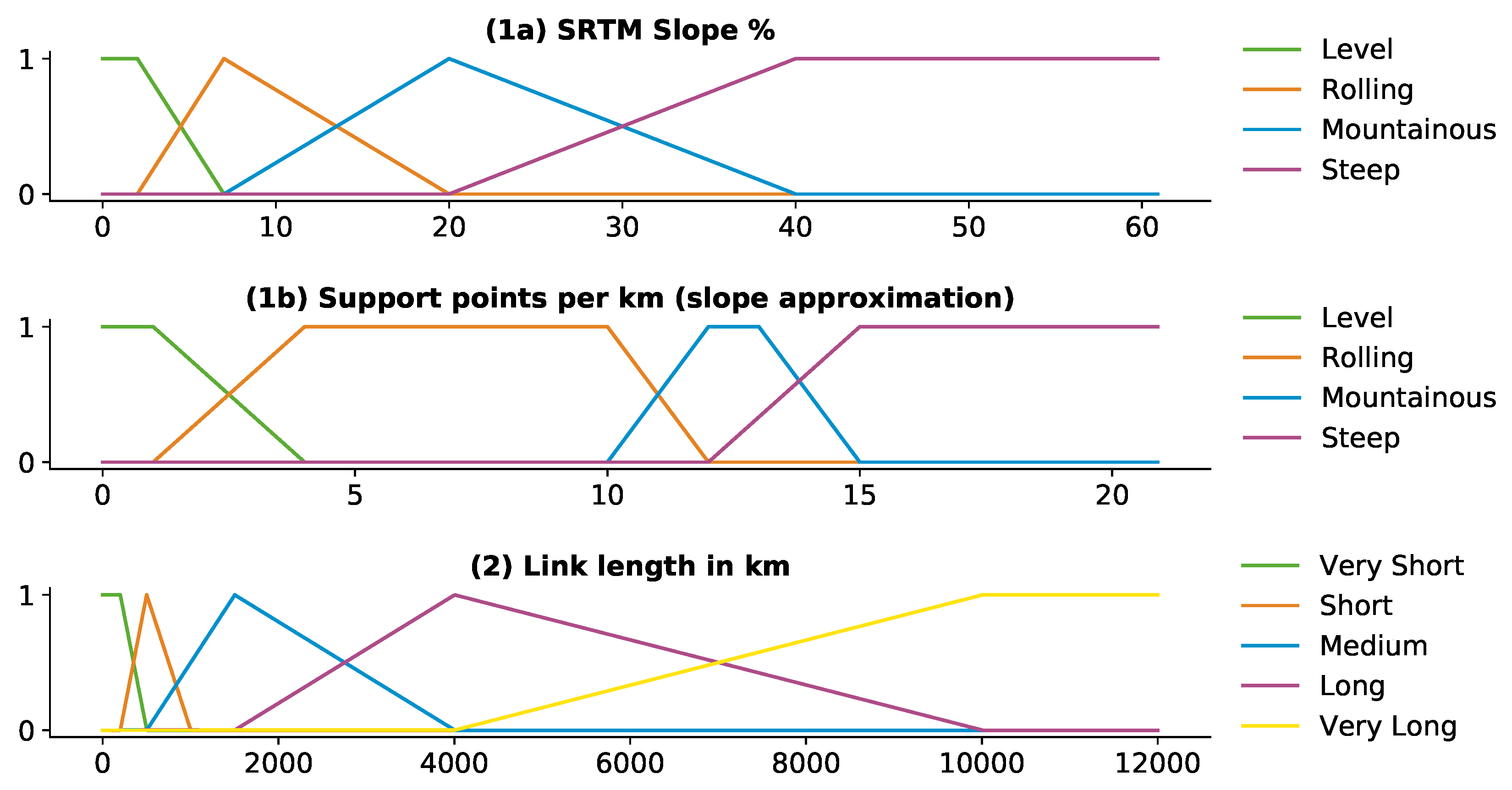
Fuzzy logic introduces the idea of partial membership. In a crisp set, members would only be members if their membership was full. In fuzzy sets, however, elements have varying degrees of memberships [35]. During the fuzzification, the MF convert crisp input and output values into fuzzy sets (Figure 3, Step 1). MF that are defined on an interval of 0 (not a member) to 1 (full member) characterize the membership of the parameters slope, link length and speed. Different types of MFs exist including triangular, trapezoidal, sigmoidal, Gaussian and bell-shaped MFs [35]. We define triangular MFs for slope and for link length which are illustrated in Figure 4.

Linguistic terms for slope include level, rolling, mountainous and steep. The linguistic terms for link length range from very short to very long. The output parameter speed varies between slow, medium and fast. In pre-studies, we have analyzed the impact of different shapes of MFs on the results. Then, we combine that with expert knowledge from literature [26,39] to obtain the presented MFs. Each FCS uses the same MF for link length and slope but different MF for speed.

According to the MF rule base, different MFs speed are defined. Depending on the input parameters road class and road surface, 10 different MF speed are designed:

• MF speed 1: Class = Motorway,
• MF speed 2: Class = Trunk,
• MF speed 3: Class = Primary & Surface = paved,
• MF speed 4: Class = Primary & Surface = unpaved,
• MF speed 5: Class = Secondary & Surface = paved,
• MF speed 6: Class = Secondary & Surface = unpaved,
• MF speed 7: Class = Tertiary & Surface = paved,
• MF speed 8: Class = Tertiary & Surface = unpaved,
• MF speed 9: Class = Unclassified & Surface = paved,
• MF speed 10: Class = Unclassified & Surface = unpaved.

For the classes Motorway and Trunk, a paved surface is assumed. In other regions, even less MF speed might be necessary as less unpaved roads exist. The ten MFs speed are designed using region specific expert knowledge about the speed distribution per road class and surface. For roads without surface information, the surface is assumed paved for the road classes Primary and Secondary and Unpaved for the road classes Tertiary and Unclassified. Specific MFs speed depending on the case study region are generated (see Section 5).

We use a Mamdani fuzzy inference system [28] which features a rule base where every rule has an antecedent (IF) part and a consequent (THEN) part (Figure 3, Step 2). Antecedents and consequents can be aggregated using an AND-operator. 20 rules have been developed with two antecedents (slope and link length) and one consequent (speed) each. Two exemplary rules are:

• IF slope is level AND link length is very long THEN speed is fast.
• IF slope is rolling AND link length is very short THEN velocity is medium AND slow.

We provide all applied rules in the form of a Python notebook via GitHub [19].

The last step of every FCS is the defuzzification (Figure 3, Step 4) which converts fuzzy output to crisp output. In our study, we tested different defuzzification methods like centroid, bisector and mean-, minimum- and maximum- of maximum. A centroid-based defuzzification (see [35]) fits our estimation best, as it results in a continuous distribution.

Note that the MFs for length and slope as well as the MF rule base and the rule base of the FCSs remain the same for every study region. Only the ten different MF speed per road class and road surface have to be adapted with expert knowledge for different regions.

5. Case Study Regions

The Fuzzy-FSE is applied exemplary for the BioBío and Maule (BM) regions in central Chile and for a part of northern New South Wales (NNSW) in Australia. In New South Wales, the study region consists of the statistical divisions Mid-North Coast, Richmond-Tweed and Northern. The study regions in Chile and in Australia are comparable in size but are at different stages of development.

In Chile, the road infrastructure is typical of a developing country. Even in populated regions, many unpaved roads exist and paved roads are often not maintained so the average speed is low compared to the same road classes in more developed countries. Australia is a developed country with a well-maintained road infrastructure. There are more high level roads in the more densely populated parts in NNSW than in comparable parts of the BM regions. This also leads to higher average speeds in all road classes which can be seen in Figure 5. In addition, the OSM dataset for NNSW is more complete and contains more additional information than the OSM dataset for the BM regions. The tag maxspeed is filled out for $22.5$% of all road kilometers in NNSW but only for $7.2$% of all road kilometers in the BM regions.

The BM regions have a characteristic topography with the coastal mountain range in the west and the Andes in the east. This leads to a wide rage of road slopes in the Chile dataset. Australia is less mountainous and has fewer roads with a high road slope. Both study regions feature large rural areas which are not densely populated. Both study regions feature more unpaved than paved roads (see

Table 2. Overview of the OSM data in the BM regions in Chile and NNSW in Australia.

	BM (Chile)		NNSW (Australia)
	km	% km	km	% km
All roads	30,349.84	100	38,956.41	100
Motorway	1624.79	5.56	882.21	2.27
Trunk	142.47	0.47	901.06	2.32
Primary	4246.53	13.99	1998.80	5.13
Secondary	3281.87	10.82	4372.52	11.23
Tertiary	15,643.31	51.55	8821.94	22.65
Unclassified	5410.94	17.83	21,979.86	56.42
Surface information	25,211.83	83.07	30,606.80	78.57
Paved	7945.20	26.18	12,406.64	31.84
Unpaved	17,266.63	56.89	18,200.16	46.72
Maxspeed information	2176.42	7.17	8756.55	22.48

) and many more low level roads than high level roads. The combination of all mentioned characteristics makes both regions ideal candidates to apply the developed Fuzzy-FSE. The transferability of the method to different rural regions is demonstrated by applying the Fuzzy-FSE to these two regions which differ in many aspects mentioned above.

Table 2 gives an overview of the OSM data for both study regions. The largest road class in Chile is Tertiary which makes up more than 50% of the road network. In Australia, most roads are in the class Unclassified. Another notable difference is the road class Trunk which is almost nonexistent in Chile but is used a lot in Australia. In both countries, most roads have surface information. The surface information is classified into two main categories paved and unpaved as more detailed surface information is rare. The tags paved, unpaved and asphalt make up $97.6$% (BM) and $82.1$% (NNSW) of the surface information. However, few roads in Australia and very few roads in Chile feature speed information which underlines the need for a speed calculation. A spatial analysis shows that many roads that feature speed information are either motorways or are located in urban regions in both study regions. In [18], we demonstrate that it is valid to exclude roads shorter than 200 $\mathrm{m}$ from the validation.

Figure 5 shows the distribution of the GD-API speed data of both study regions and for the different road classes. Average speeds per class are calculated from the GD-API to compare against the estimations of the Fuzzy-FSE. In the GD-API dataset for the BM regions, the average speeds are: 94 km/$\mathrm{h}$ (Motorway), 58 km/$\mathrm{h}$ (Trunk), 61 km/$\mathrm{h}$ (Primary), 45 km/$\mathrm{h}$ (Secondary), 34 km/$\mathrm{h}$ (Tertiary) and 26 km/$\mathrm{h}$ (Unclassified). In the NNSW dataset average speeds are: 99 km/$\mathrm{h}$ (Motorway), 80 km/$\mathrm{h}$ (Trunk), 76 km/$\mathrm{h}$ (Primary), 68 km/$\mathrm{h}$ (Secondary), 56 km/$\mathrm{h}$ (Tertiary) and 38 km/$\mathrm{h}$ (Unclassified).

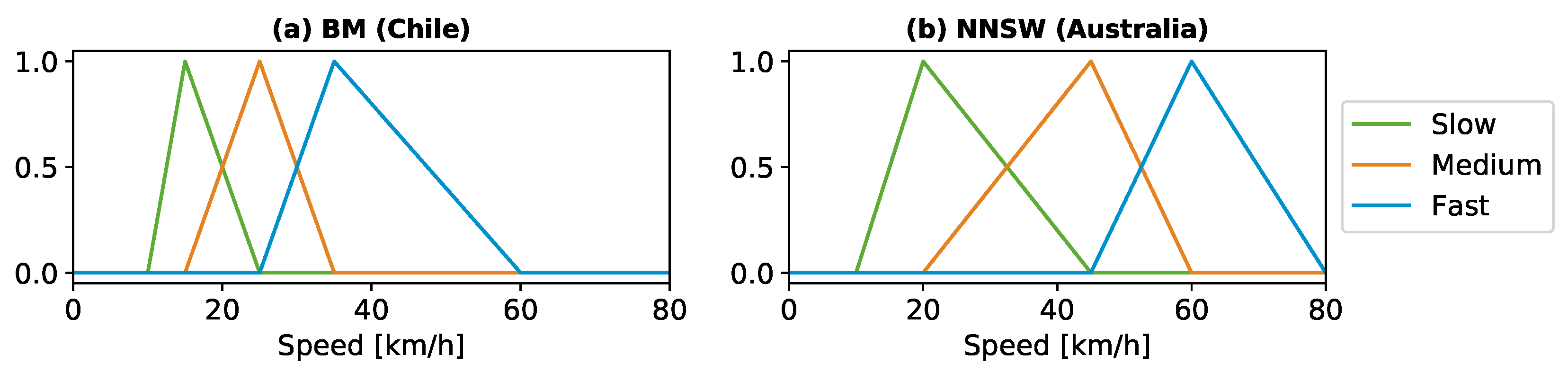
As described in Section 4, ten MFs for speed are defined for every study region. The MF speed are defined manually using expert knowledge about the regions road conditions and speed distribution. In this case, the expert knowledge is taken from the distribution of the GD-API speed data. Two exemplary MF speed, one for the BM region and one for NNSW, for the class Tertiary and for an unpaved surface are shown in Figure 6. The definition of all MF speeds for both study regions is provided via GitHub [19].

Of the 17,809 (BM)/21,977 (NNSW) roads considered for the evaluation, approximately 12% (BM)/4% (NNSW) are excluded due to the errors described in Section 3.3. The errors occur when the road distance between the OSM and the GD-API data differ in more than 20% (50% (BM)/28% (NNSW) of the errors) and when the start or endpoints differ in more than 50 $\mathrm{m}$ (46% (BM)/69% (NNSW) of the errors). In 60 (BM)/20 (NNSW) cases the GD-API respond with an error.

6. Results

We apply the Fuzzy-FSE on both study regions in two modes: Once with only OSM data, using the support points per kilometer as an approximation for road slope. The other mode calculates road slope percentages with SRTM data and uses OSM for the rest of the input parameters. Both applications are tested once with all roads included and once with only the roads having a surface information. As described in Section 4, when all roads are included, the ones without surface information are assigned a default surface depending on the road class. Additionally, the influence of link length on the results is analyzed by testing the effect of including first all roads longer than 200 $\mathrm{m}$, then all roads longer than 400 $\mathrm{m}$ and finally all roads longer than 600 $\mathrm{m}$. A fixed speed profile that consists of the average speed for each class of the GD-API speed data is calculated as a baseline.

Table 3. Comparison of the R² and RMSE (Root mean square error) of the BM regions (Chile) for all links over 200 $\mathrm{m}$, 400 $\mathrm{m}$ and 600 $\mathrm{m}$, respectively. The maximum value of each row with only OSM data and with OSM and SRTM data is highlighted in bold.

		Google	OSM		OSM + SRTM
		Baseline	All Roads	Roads with Surface	All Roads	Roads with Surface
> 200 m	R2 [%]	66.66	67.90	61.31	67.73	61.00
	RMSE [km/h]	12.74	13.29	13.60	12.92	13.12
> 400 m	R2 [%]	72.09	73.00	67.16	73.48	67.55
	RMSE [km/h]	11.79	12.49	12.83	11.69	11.95
> 600 m	R2 [%]	73.64	75.12	70.04	75.66	70.53
	RMSE [km/h]	11.48	12.00	12.13	11.08	11.28

shows the results for the BM regions for all tested modes. Both applications of the Fuzzy-FSE perform better than the baseline. The performance increases with the length of the links. The results of the Fuzzy-FSE for the BM regions are much better when all roads are included, instead of only the roads with surface information. The performance of the Fuzzy-FSE with the input from both OSM and SRTM data are approximately equal to the Fuzzy-FSE using only OSM data. The best result for the BM regions (R²: $75.66$%, Root mean square error (RMSE): per-mode=symbol $11.08$ $\mathrm{k}$$\mathrm{m}$/$\mathrm{h}$) is achieved by taking both OSM and SRTM data as input and only considering all roads longer than 600 $\mathrm{m}$.

The results for NNSW in Australia are presented in

Table 4. Comparison of the R² and RMSE of NNSW (Australia) for all links over 200 $\mathrm{m}$, 400 $\mathrm{m}$ and 600 $\mathrm{m}$, respectively. The maximum value of each row with only OSM data and with OSM and SRTM data is highlighted in bold.

		Google	OSM		OSM + SRTM
		Baseline	All Roads	Roads with Surface	All Roads	Roads with Surface
> 200 m	R2 [%]	51.10	57.67	61.73	57.56	61.56
	RMSE [km/h]	16.83	16.81	15.92	16.45	15.77
> 400 m	R2 [%]	57.68	64.90	69.04	65.12	69.28
	RMSE [km/h]	16.00	15.62	14.51	14.92	13.99
> 600 m	R2 [%]	58.35	66.22	70.29	66.50	70.57
	RMSE [km/h]	16.02	15.35	14.21	14.58	13.61

. The Fuzzy-FSE performs significantly better than the baseline with an R² which is between 6% to 12% higher than the one of the baseline. Similar to the results of the BM regions, the performance of both Fuzzy-FSE modes is approximately the same. Contrary to the BM regions, the results are better if only the roads with surface information are considered. Using both OSM and SRTM data as input and only evaluating the links with surface information and over 600 $\mathrm{m}$ length leads to the best result with an R² of $70.57$% and an RMSE of per-mode=symbol $13.61$ $\mathrm{k}$$\mathrm{m}$/$\mathrm{h}$.

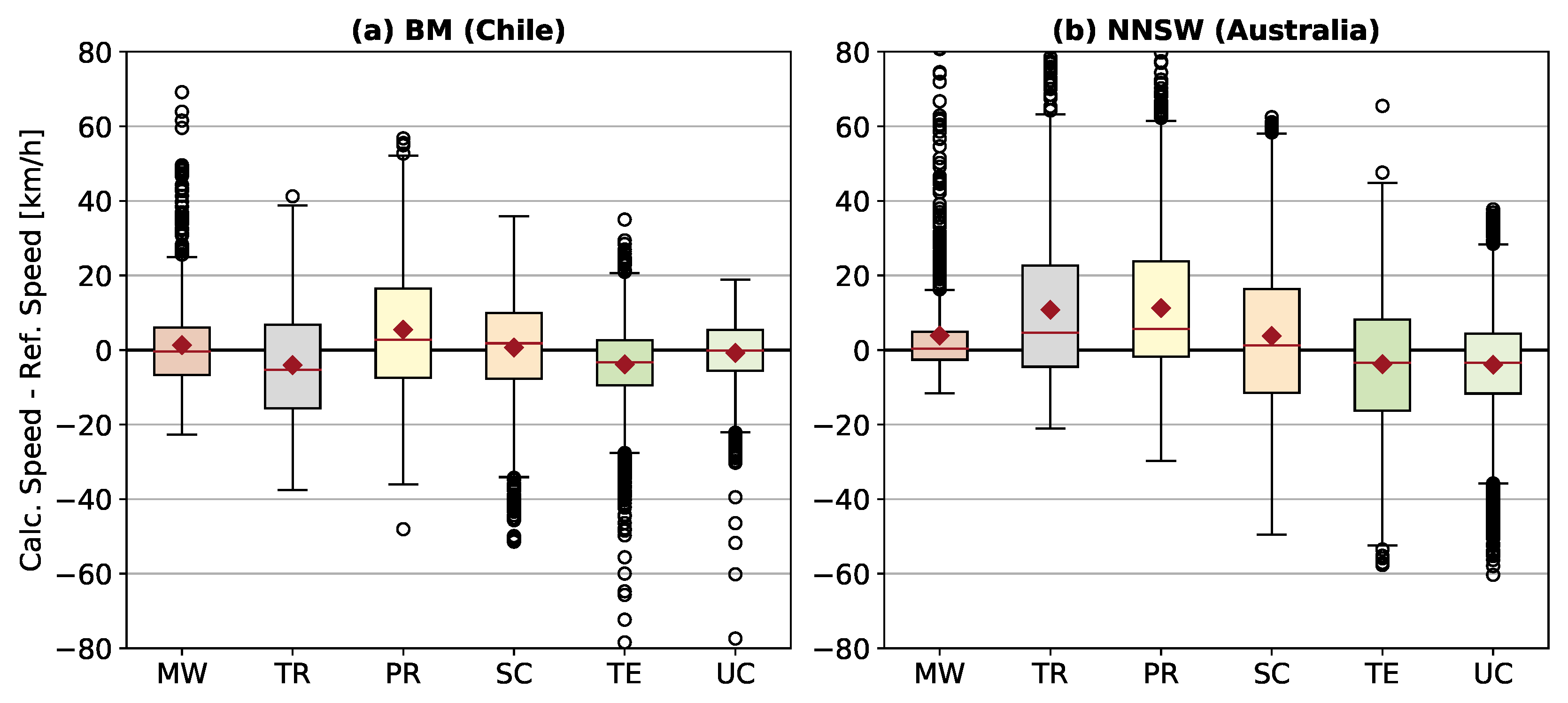
Figure 7 shows the distribution of the difference between the calculated speed and the reference speed per road class for both study regions. The speed values include all links longer than 200 $\mathrm{m}$ and are calculated with both OSM and SRTM as input data. In NNSW, the differences between the calculated and the reference speed are generally higher than in the BM regions. In the BM regions, the classes Motorway, Tertiary and Unclassified perform best. The classes Motorway and Unclassified feature the best results in NNSW.

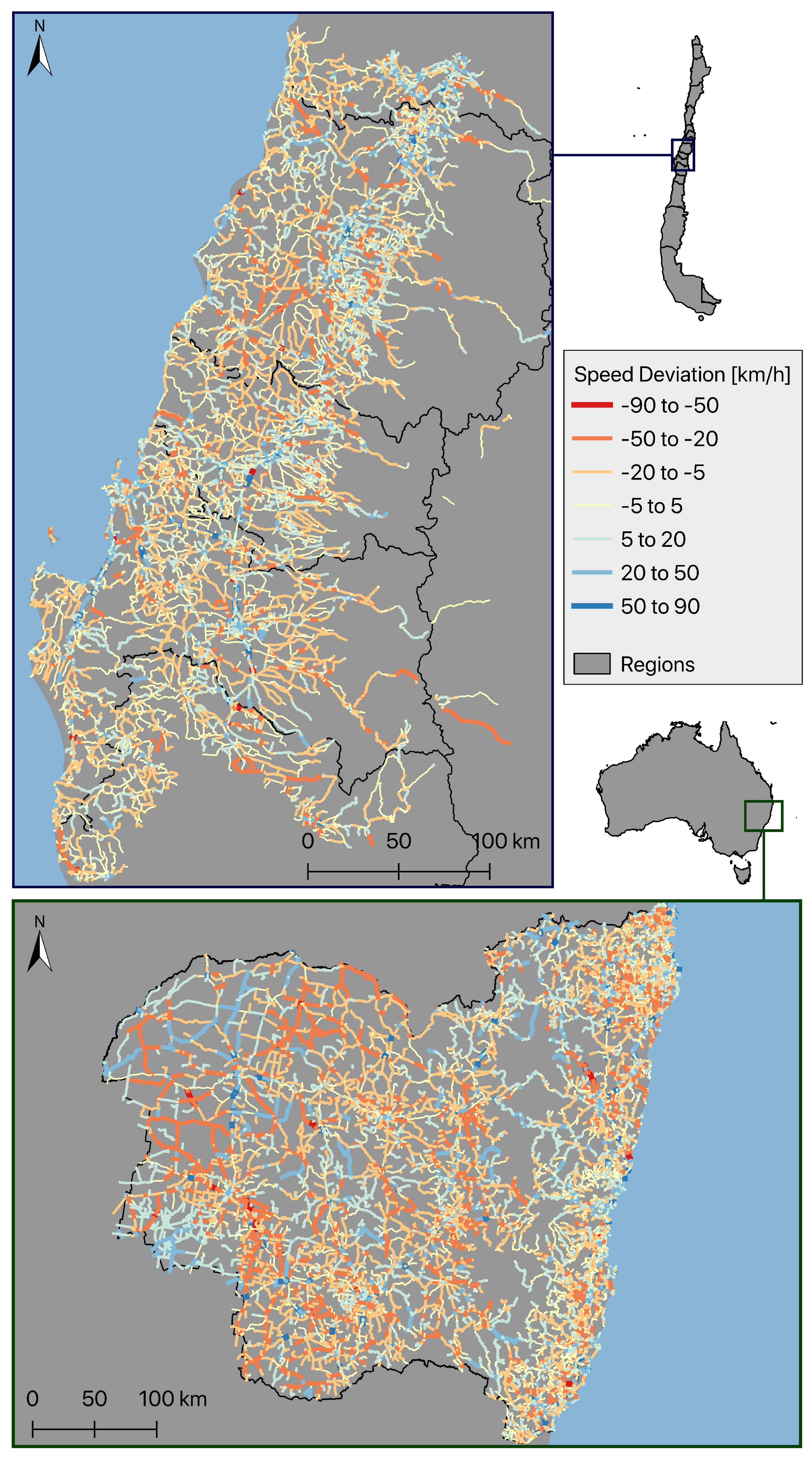
A map of the speed deviation with all roads over 200 $\mathrm{m}$ and both OSM and SRTM data as input is illustrated in Figure 8. Generally, the geographic distribution of the speed deviation is consistent in both study regions. However, in the west of the study region in Australia, some roads exist that are both significantly under- and overestimated. Within the urban centers, the Fuzzy-FSE mostly calculates higher speed values than the GD-API.

7. Discussion

Our developed Fuzzy-FSE is applied for both study regions in various modes. This allows for a detailed analysis of the different results. In this section, we discuss and interpret the results shown in Section 6. We concentrate on the performance of the Fuzzy-FSE rather than detailed regional analyses. In the discussion, we focus on the performance of: the Fuzzy-FSE versus the baseline, including only OSM data versus adding also SRTM data, analyzing all roads or only the ones with surface information and evaluating different link lengths.

The calculated baseline represents the current state of the art. As explained in Section 2, most routing applications use fixed speed values per road class to calculate the cost factor travel time. The baseline we calculate is most likely more adapted to the regions characteristics than other speed profiles as it uses the average speed of the GD-API, which is an information most routing engines lack. In comparison to the baseline, the developed Fuzzy-FSE performs better for both study regions. For NNSW, the improvement is much more significant than for the BM regions. This may be caused from the differences in the datasets. According to the range of the GD-API speed data (see Figure 5), the speed range in NNSW is considerably larger than in the BM regions. The smaller the range of the speed values, the better it can be approximated by an average speed value. In NNSW, the large speed range can be estimated significantly better with the Fuzzy-FSE than with the baseline as it is able to provide a continuous range of speed values. On the other hand, the overall performance of all estimations presented in this study is better in the BM regions. This is also caused by the large speed range in NNSW as even the Fuzzy-FSE cannot cover the entire speed range.

We analyze two modes to calculate speed which differ in the input data for road slope. The first mode uses only OSM data, while the second mode adds SRTM data. Although the R² are more or less equal for both modes, the RMSE is smaller when SRTM data are included. The road slope approximated by calculating support points per kilometer is less accurate as a curvier road does not always signify higher slopes. In addition, the vector shapes in OSM may often be more straight than the actual road as contributors map imprecisely. Still, the results show that accurate speed estimations can be calculated by the Fuzzy-FSE using only OSM data with no additional data source.

The effect of road surface information in OSM is also analyzed. We compare the performance of the Fuzzy-FSE with all roads to the results which include only the roads which feature surface information in OSM. The results in both study regions are contrary. The initial expectation was that including only the roads with surface information should be better than considering all roads. This expectation is confirmed in NNSW. However, in the BM regions, taking all roads and thus including the default surface values per road class (see Section 4) results in significantly better performance of the Fuzzy-FSE. We assume that this might stem from a possible bad quality of the road surface data in the BM regions. Considering the study region NNSW, the Fuzzy-FSE performs worse without surface information but still are at least 6% better than the baseline.

Furthermore, we evaluate the effect of link length on the performance of the Fuzzy-FSE. The resulting speed values are less accurate for shorter links than for longer links. A large part of this is due to the insecurities of the GD-API speed data which are described in Section 3.3. Additionally, a false speed value has a smaller effect for a shorter road than for a longer one as it is later multiplied by the distance to obtain travel time. Therefore, it is valid to only consider longer roads for an evaluation of the Fuzzy-FSE.

The Fuzzy-FSE estimates some road classes better than others. Comparing the ranges of the speed values per road class (Figure 5) with the difference between calculated speeds and reference speeds (Figure 7), a correlation can be seen. The larger the range of speed values, the larger is the distribution of the speed difference. Considering the real world, a motorway features a mostly homogeneous speed, generally at least two lanes and little slope variation. Primary roads, however, represent a very inhomogeneous class with some roads having two lanes and others that may not even be asphalted. The unclassified roads are again more homogeneous with mostly unpaved roads where faster speeds are not possible.

The presented Fuzzy-FSE is designed for rural application. In urban and suburban regions traffic, the number of turns or local speed limits play a much bigger role for the speed estimation than surface, link length, slope and road class. In particular, traffic is a very big factor in the urban environment that cannot be estimated from OSM data only. Traffic estimations require data on road capacity and volume of vehicles per day or hour. Furthermore, traffic is a factor that is highly variable in time with peak hours in the morning and evening and almost no traffic at nighttime. Thus, the inclusion of traffic in the Fuzzy-FSE is not possible with the available data and therefore not the objective of this study. In addition, speed limits in urban regions are not considered in the definition of the MF speed. The Fuzzy-FSE is not able to differentiate between urban and rural regions because the OSM dataset contains no information on population density. Therefore, estimated speed values in urban centers should be treated with caution. Furthermore, roads in urban regions often already feature speed information, as in the OSM datasets the tag maxspeed is filled out more often in urban centers than in rural regions. This reduces the need to calculate average speeds for the urban road infrastructure.

In comparison to our previous study [18], we analyze the speed values instead of travel times. As it turns out, the evaluation of travel time provides little information about the quality of the estimation. There are very few high values which make up the upper three quarters of the range. This leads to misleading high R²-values. The FCS developed in [18] performs worse or equal to the baseline, both analyzing speed values and travel times.

The GD-API data are applied as reference data for the Fuzzy-FSE. As mentioned in Section 3.3, some inconsistencies exist between the Google Maps data and the OSM data. The error statistics in Section 5 emphasize this issue. Some errors cannot be caught and are treated as reference data, which falsifies the results. Thus, the GD-API data are only suitable to some extent as valid reference data. However, other reference datasets that are readily available and feature worldwide coverage do not exist.

Finally, if the developed Fuzzy-FSE is supposed to be applied to a different region, its limitations have to be considered. The Fuzzy-FSE does not consider traffic or other temporal factors like visibility or wildlife activity at certain times of the day. Therefore, the calculated speed values have to be considered as rough estimates rather than exact values. However, better estimates would need more input data than just OSM data. As discussed above, it is also not applicable to urban regions as on the one hand the factors in urban environments are different and cannot be taken from OSM data. On the other hand, different MF speeds would be needed for each road class inside the cities as speed limits are much lower than outside the cities. Thus, the Fuzzy-FSE is applicable to regions where the road network mainly consists of rural streets or as part of a tool that has a different calculation method for urban average speed values. One major limitation stems from the nature of fuzzy control and is the dependence of the Fuzzy-FSE on the expert knowledge. It is very sensitive towards false knowledge but that can be detected by comparing the results to adequate ground truth data. Generally, the Fuzzy-FSE is able to include more parameters, but a FCS does not scale well as the number of required rules rises approximately as the product of number of categories of the input parameters.

8. Conclusions and Outlook

We develop a Fuzzy-FSE that employs multiple FCSs to estimate average speed from the parameters road class, road slope, road surface and link length. These parameters can all be extracted or calculated from the open source and worldwide available dataset OSM. The inclusion of SRTM data to estimate road slope is tested but improves the results only slightly. The GD-API data serves as reference data and as foundation for the baseline calculation. Exemplary applications on case studies in the BioBío and Maule regions in Chile and north New South Wales in Australia demonstrate the applicability in two distinct regions which differ in their state of development and in their quality of OSM data. Average speed values are estimated better compared to existing methods and compared to our previous study in [18].

The developed Fuzzy-FSE offers the advantages of Fuzzy Control. It includes fuzzy input parameters and a reasoning process of a human operator. In contrast to machine learning approaches, training data are not needed as it is based on expert knowledge. However, it has to be considered that the ability of a FCS to perform well highly depends on its design. Thus, the Fuzzy-FSE is much more susceptible to false assumptions than, for example, a machine learning model would be.

A major advantage of the developed Fuzzy-FSE is the worldwide transferability for the average speed estimation in rural regions. When applying the Fuzzy-FSE to a different region, it has to be considered that the Fuzzy-FSE is not designed to estimate average speed in urban regions. A region that contains both rural and urban regions would need a different methodology for the urban part of the region in addition to the Fuzzy-FSE. To estimate average speed values for a different region, only the MF speed has to be adapted using expert knowledge about the new study region. Furthermore, the Fuzzy-FSE is able to estimate average speed only with OSM data itself. This enables a very quick application without much preprocessing. Both the fixed speed limit baseline and the Fuzzy-FSE perform best in regions where the speed distribution per road class is relatively uniform. However, another advantage of the Fuzzy-FSE is that it is still able to obtain good results even if the range of speed values per road class is large. This is where, in comparison, fixed speed limits fail.

The findings of this study can be used in many different applications. Most routing engines could include the Fuzzy-FSE rather than using fixed speed profiles for every road class. Many studies on critical road infrastructure rely on commercial travel time data as a cost factor in the road network. They could benefit very much from estimated average speed values in rural regions.

In future research, we aim at applying data-driven methods like different machine learning models for the estimation of average speed. In addition, a least square optimization could find the optimal membership functions as well as the rule set to best fit the FCS to the ground truth. The performance of these methods can then be compared to the results of the Fuzzy-FSE. The Fuzzy-FSE itself is extendable as data from additional data sources could introduce parameters with a temporal variability like visibility or traffic. Other methods to approximate road slope like using the relationship between the driving speed and the turning radius can also be implemented. Furthermore, it could be investigated if it is possible to adapt the Fuzzy-FSE to urban circumstances with different MF speed and possibly different input parameters. The result would then consist of two different Fuzzy-FSE: one for urban and the other for rural environments. In addition, more analyses could be performed including different study regions with different qualities of OSM data. In particular, including more densely populated countries like Germany could be interesting. The application in more and different study regions would enable a detailed sensitivity analysis towards the input parameters.