Joint Simulation of Spatially Correlated Soil Health Indicators, Using Independent Component Analysis and Minimum/Maximum Autocorrelation Factors


Abstract
1. Introduction
2. Materials and Methods
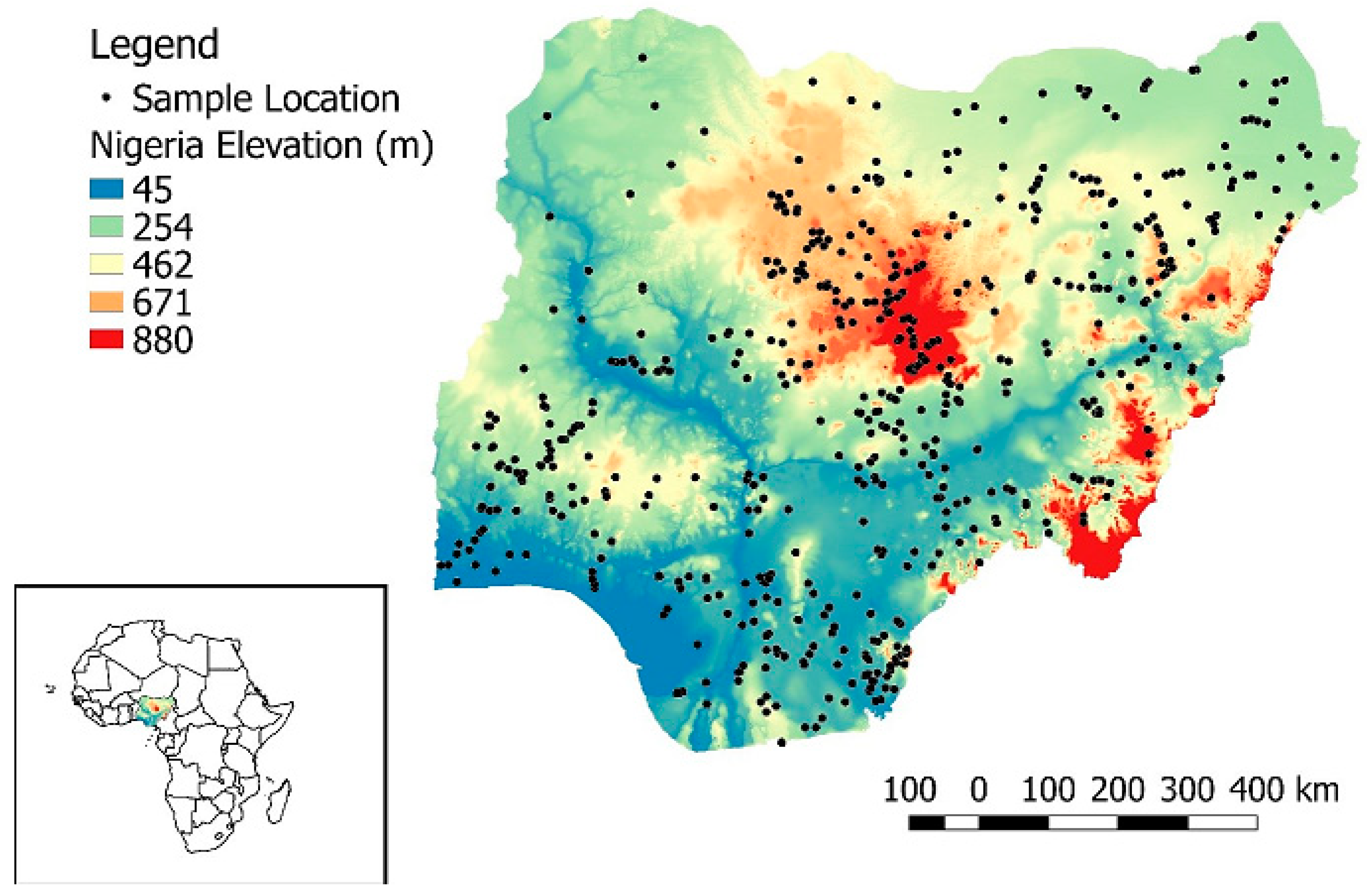
2.1. Description of the Dataset and Study Area
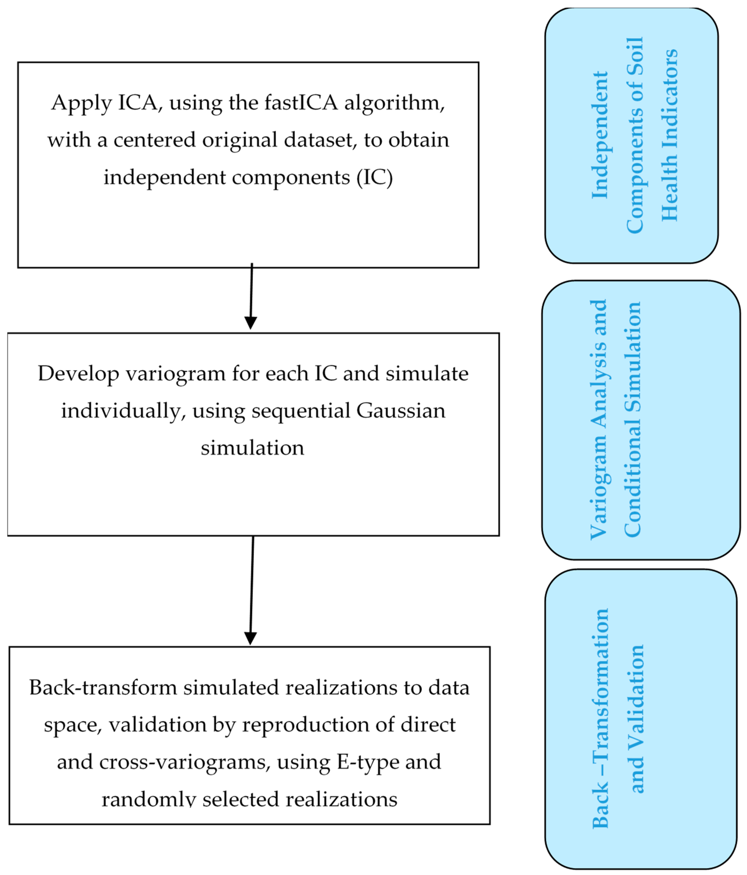
2.2. ICA
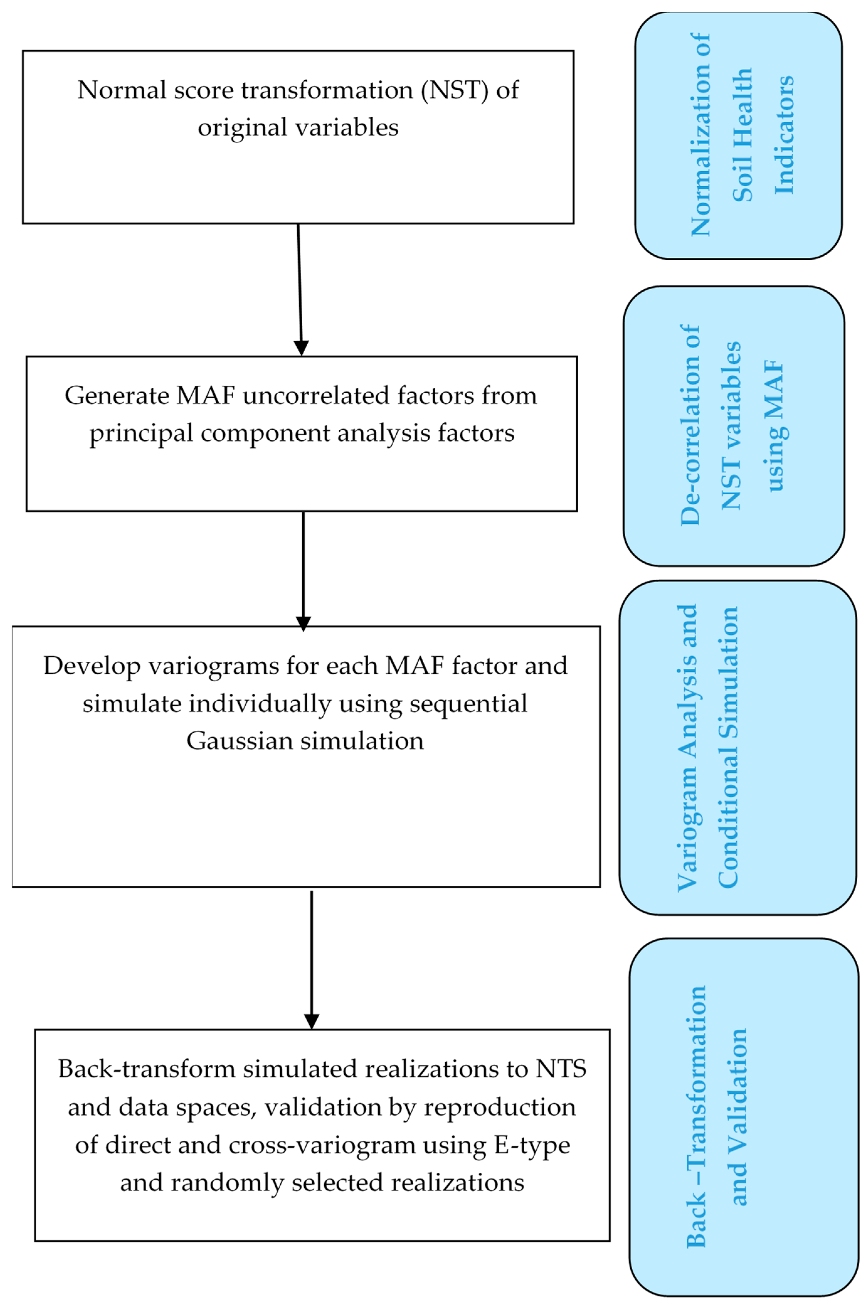
2.3. MAF
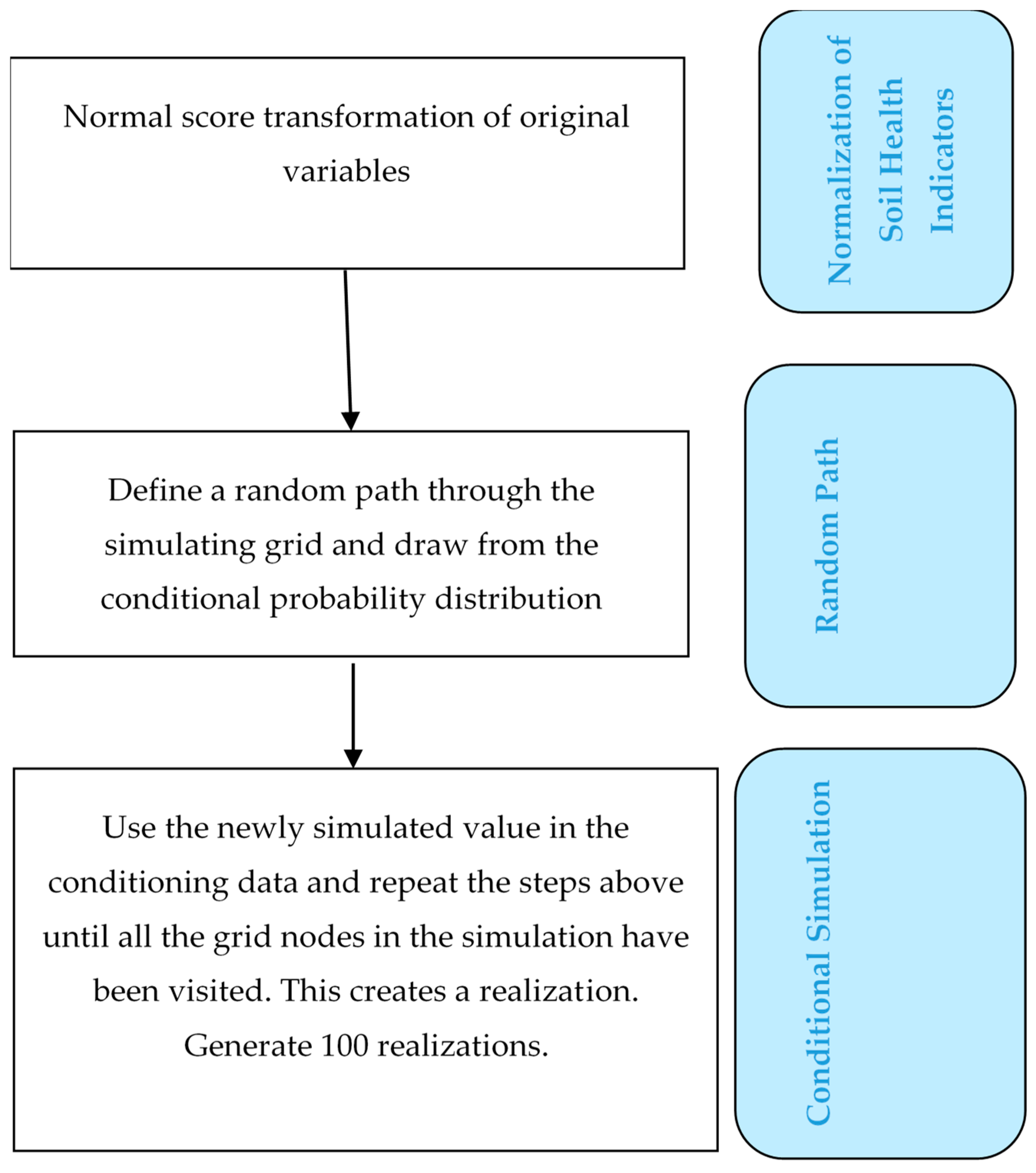
2.4. SGS
2.5. Verification and Validation of MAF and ICA Algorithms in the Joint Simulation of Soil Health Indicators
- (a)
- The test for spatial orthogonality assesses how well the methods (i.e., MAF and ICA) orthogonalize the variogram matrices at various lag distances [29,52]:
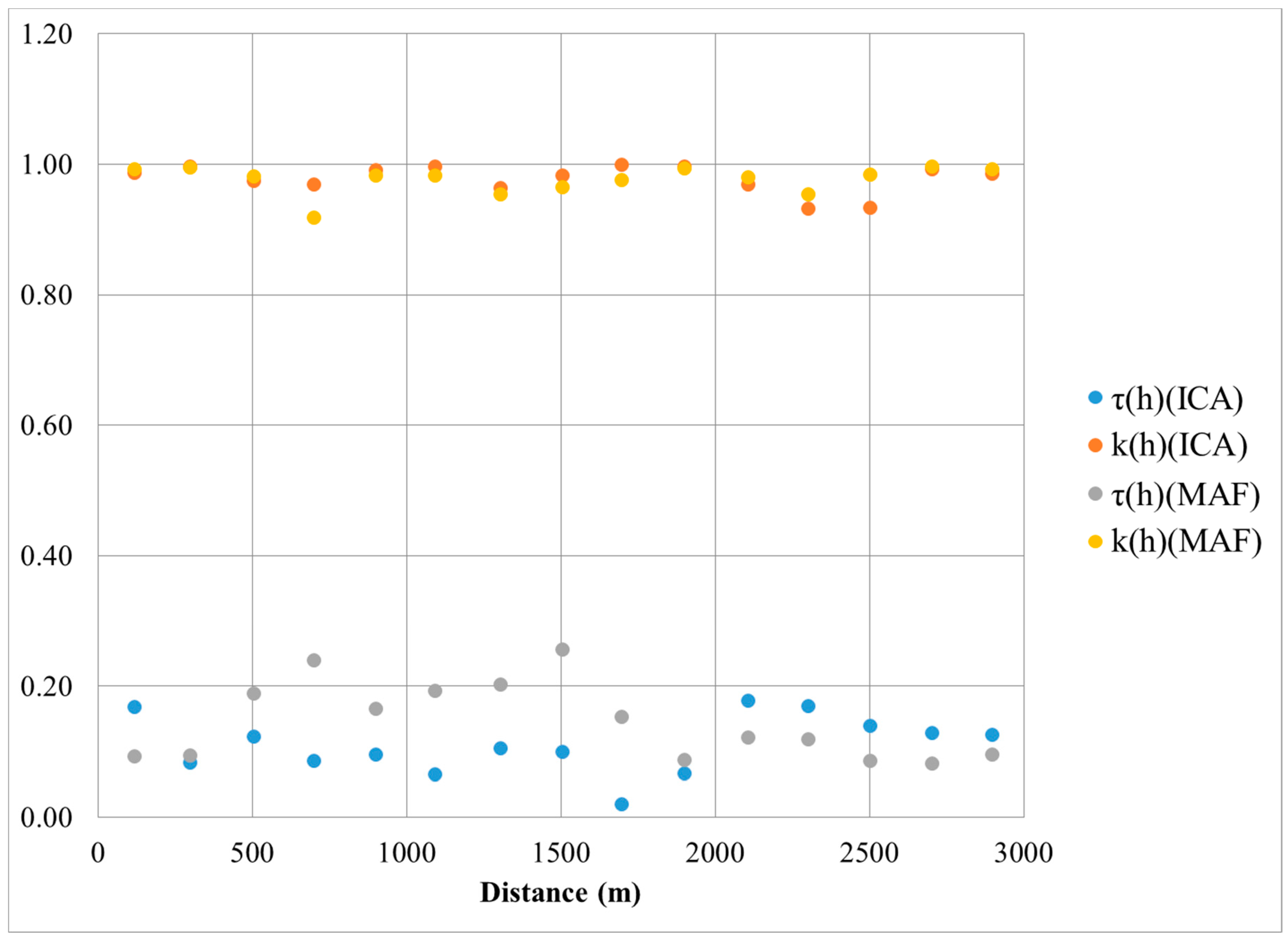
- The relative deviation from orthogonality can therefore be defined as:where γMAF (h: k, j) is the cross-variogram of the MAF or ICA, and γMAF (h: k, k) is the direct variogram of the MAF or IC. M is the variogram matrices length. For perfect spatial orthogonally, τ(h) = 0.
- The spatial diagonalization efficiency is a measure that compares the sum of squares of off-diagonal elements in ΓMAF (h) with those of the attribute of the semi-variogram matrix ΓY (h):where γY (h: zk, zj) represents the cross-variograms of the original variables. For perfect orthogonality, k(h) = 1.
- (b)
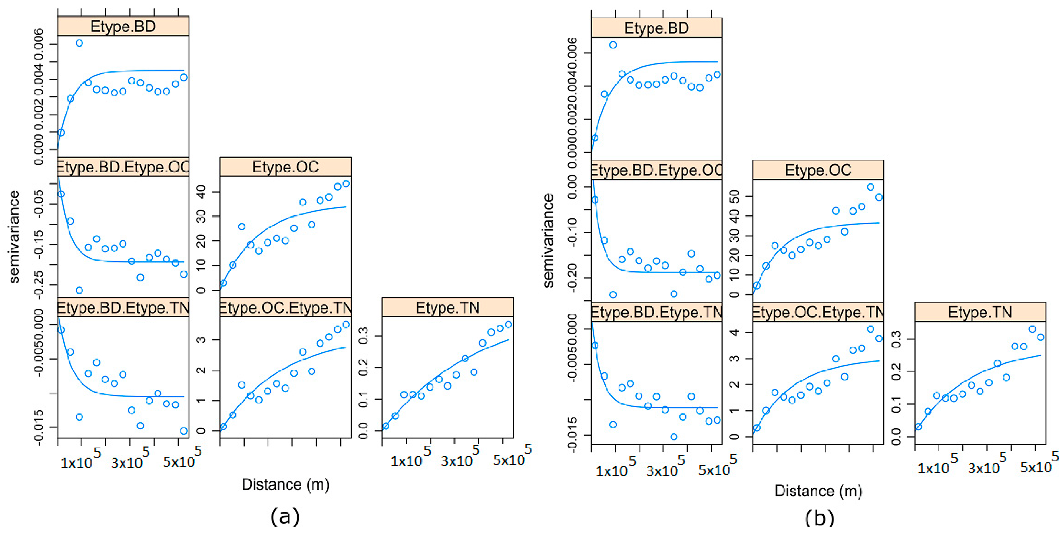
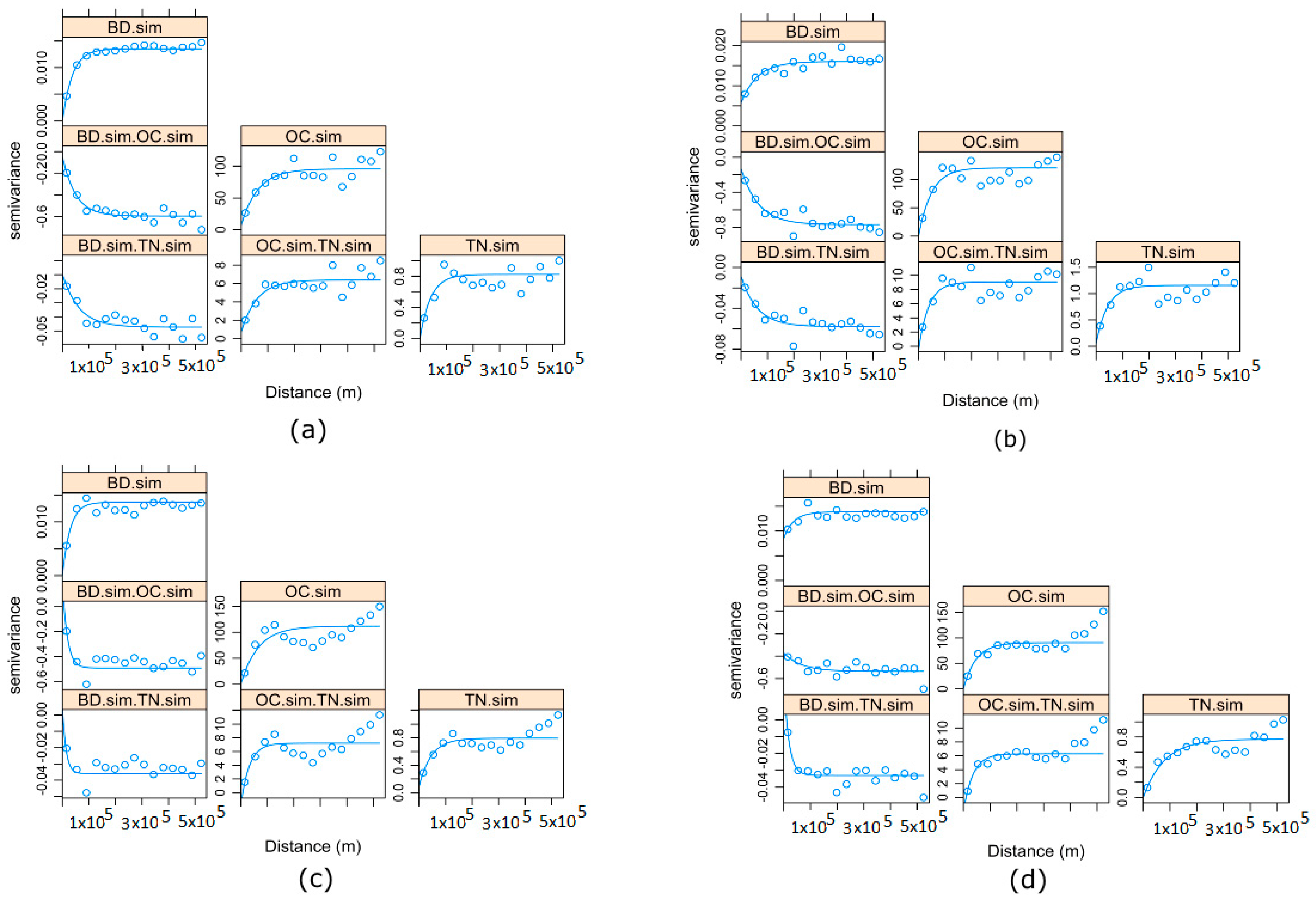
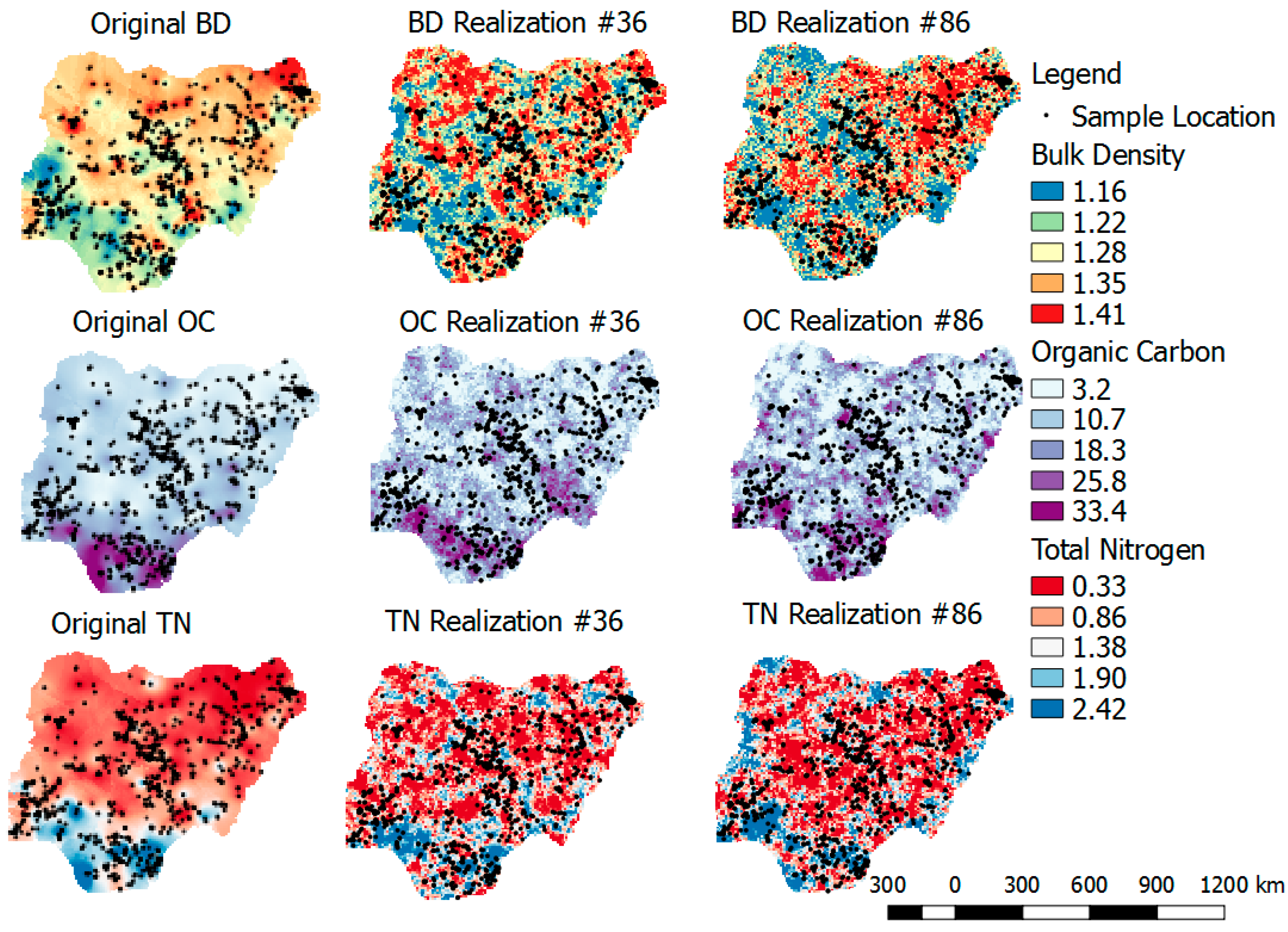
- Reproduction of direct and cross-variograms, using the average of realizations and randomly selected realizations:For both algorithms to be valid, the direct and cross-variograms of the original variables should be reproduced by the back-transformed simulated realizations. A total of 100 realizations would be averaged (in data space). This is defined as E-type, where E is the “conditional expectation” of realizations (i.e., average estimate of realizations) [51,53], and their direct and cross-variograms would be compared with those of the original variables for both MAF and ICA. In addition, randomly selected back-transformed simulated realizations would be compared. The goal is to ensure these realizations reproduce the spatial structure and characteristics of the original variable;
- (c)
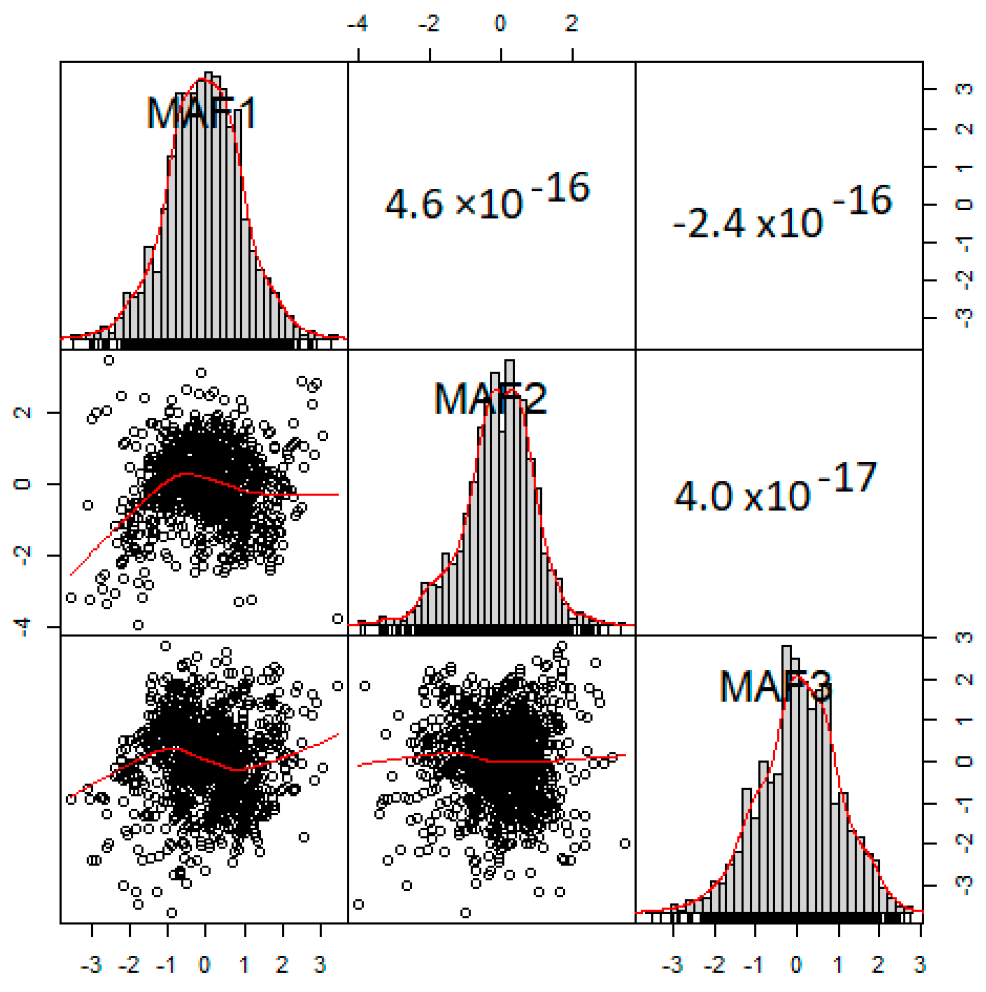
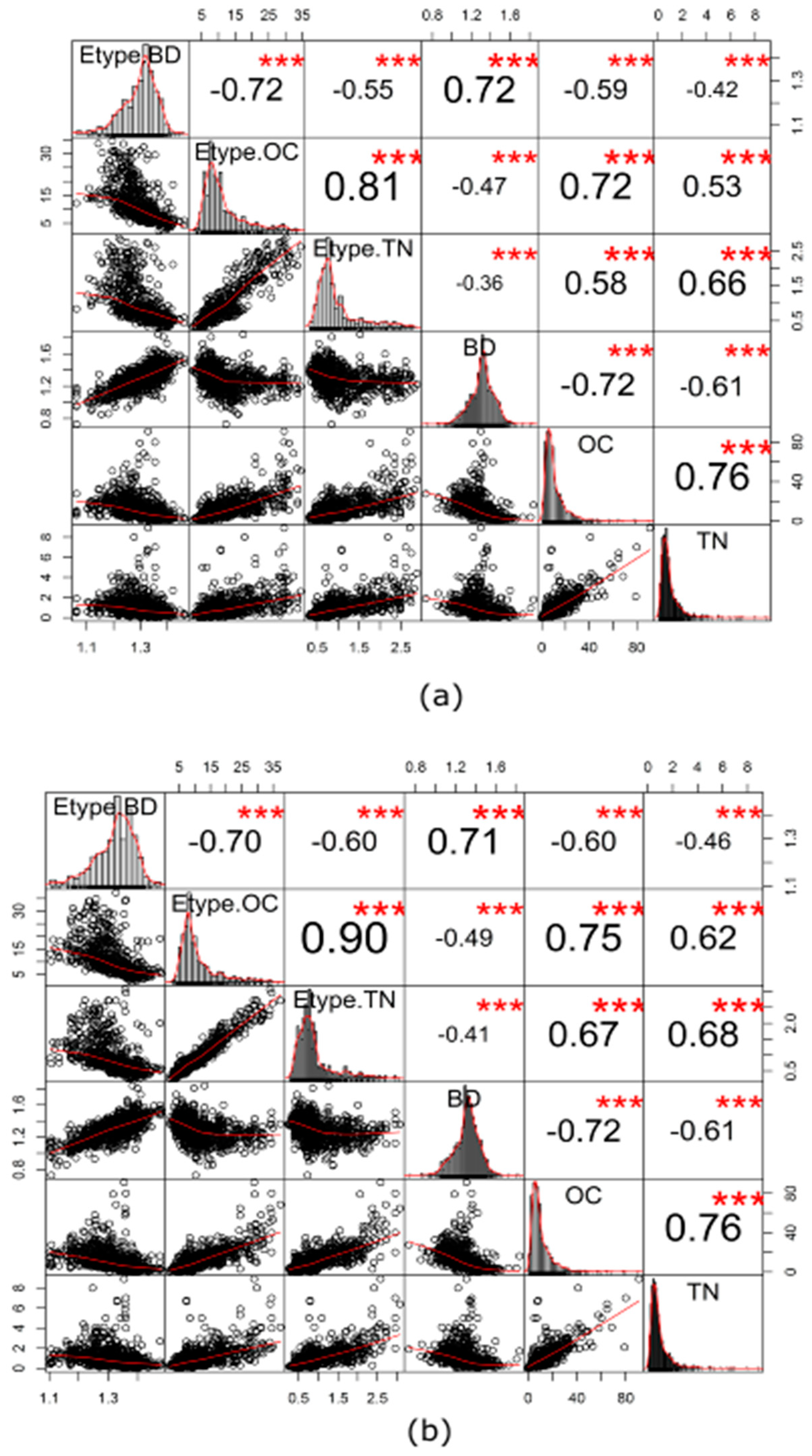
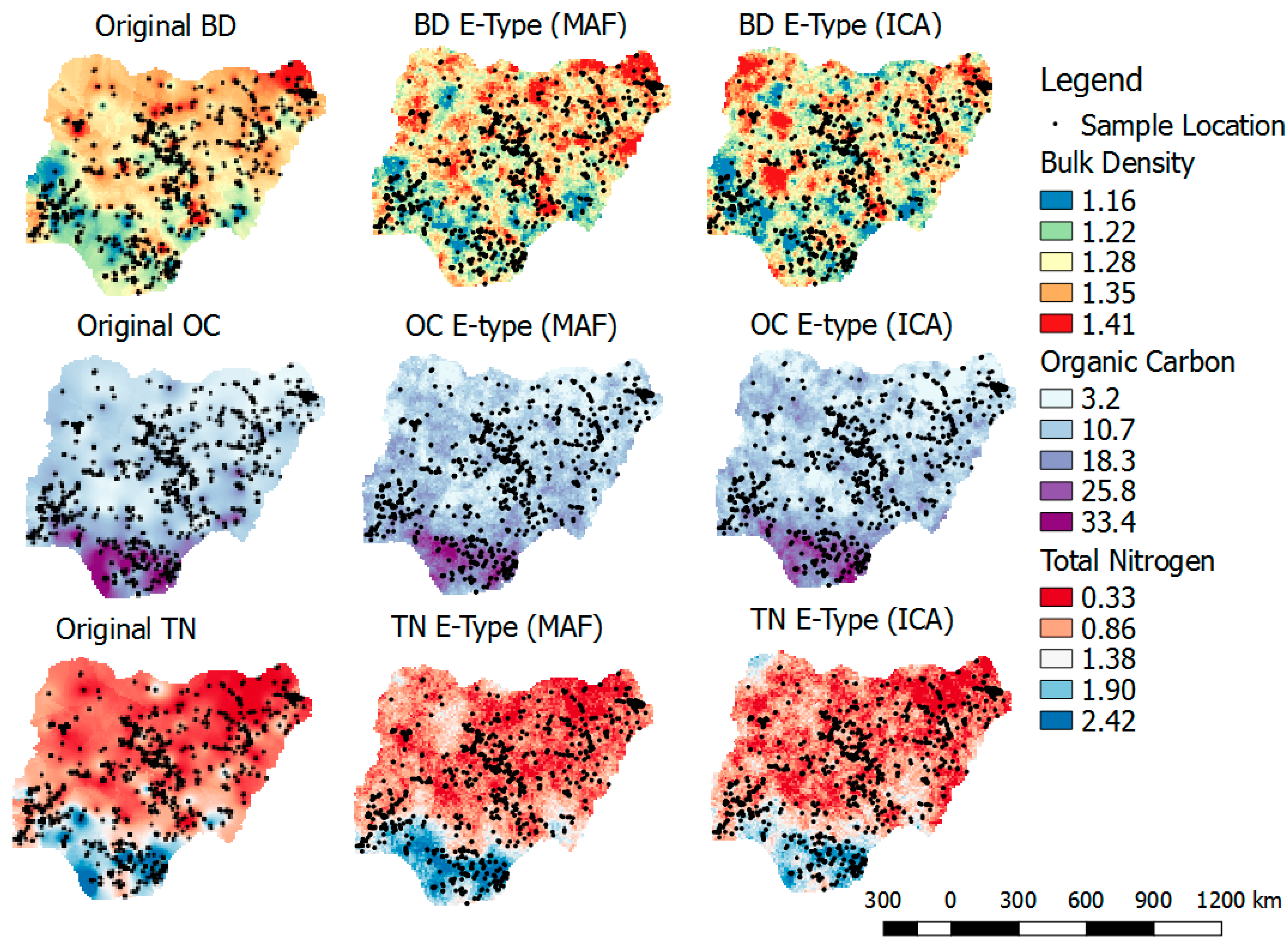
- Reproduction of the original distribution, cross-correlation, and spatial pattern:Cross-correlation between E-type of the back-transformed realizations and original variables would be compared. The reproduction of the histogram of the original variables would also be explored. In addition to the quantitative comparison above, visual inspections in the form of the reproduction of the spatial pattern of the original variable and back-transformed simulated realizations would be considered. This is to ensure consistency and to validate spatial dependency within the variables and also to guarantee the spatial relationship among the variables.
3. Results and Discussion
3.1. MAF and ICA Results
- (a)
- Performance evaluation if MAF factors and ICA components are orthogonal for all lag distances, using the measure of spatial orthogonality;
- (b)
- Reproduction of both direct and cross-variograms of original SHIs, using an average of 100 back-transformed simulated realizations for both MAF and ICA;
- (c)
- Reproduction of direct and cross-variograms of original SHIs, using randomly selected back-transformed simulated realizations for both MAF and ICA; and
- (d)
- Exploration of the distribution (histogram), cross-correlation, and spatial pattern of original SHIs and back-transformed simulated realizations.
3.2. Performance Evaluation of MAF and ICA Decorrelation, Using the Spatial Orthogonality Measures
3.3. Reproduction of Original Direct Variograms
3.4. Reproduction of Direct and Cross-Variograms, Using E-Type of Simulations
3.5. Reproductions of Original Variograms and Cross-Variograms, Using Randomly Selected Realizations
3.6. Reproduction of Distributions, Cross-Correlation, and Spatial Patterns of Original Variables by E-Type
3.7. Importance of Uncertainty in Simulating Spatially Correlated Variables and Implications for Best Management Practices (BMP) in Sustainable Management
4. Conclusions and Recommendation
- (a)
- Comparative analysis between the two methods revealed no marked differences in their performance. However, NST is necessary before MAF transformation. In the case of ICA, it was unnecessary to perform NST before transformation. In other words, NST was only used for IC while generating equally probable realizations via SGS. Therefore, IC can be used directly in other applications that do not require SGS simulation;
- (b)
- Both techniques satisfy the two criteria for spatial orthogonality suggested by Tercan (1999). These are absolute deviation from diagonality () and relative deviation from diagonality (), with ideal values of approximately 0 and 1, respectively. In other words, the MAF and ICA should be spatially orthogonal with a correlation at zero for all distances before they are used in SGS;
- (c)
- If MAF and ICA are simulated independently, both methods only require one direct variogram for each factor/component. This is in contrast to the three direct and three cross-variograms that would be needed if a traditional approach such as the model of co-regionalization was used. In other words, both MAF and ICA correctly reproduced the direct and cross-variograms of the original variables despite the variograms of MAF factors and ICA being simulated independently;
- (d)
- The back-transformed simulated variogram realizations were comparable with the original variables of each variable. Moreover, the E-type, which is the average of 100 realizations, compared well with the original variables. The cross-correlation, histograms, and spatial pattern of the back-transformed realizations, using the E-types, were correctly reproduced.
Funding
Acknowledgments
Conflicts of Interest
References
- Greiner, L.; Nussbaum, M.; Papritz, A.; Zimmermann, S.; Gubler, A.; Grêt-Regamey, A.; Keller, A. Uncertainty indication in soil function maps—Transparent and easy-to-use information to support sustainable use of soil resources. Soil 2018, 4, 123–139. [Google Scholar] [CrossRef]
- Bouma, J. Soil science contributions towards Sustainable Development Goals and their implementation: Linking soil functions with ecosystem services. J. Plant Nutr. Soil Sci. 2014, 177, 111–120. [Google Scholar] [CrossRef]
- Blum, W.E.H. Role of soils for satisfying global demands as defined by the U.N. Sustainable Development Goals (SDGs). In Rattan. Horn, Rainer; Takashi, K., Ed.; Schweizerbart’sche Verlagsbuchhandlung: Stuttgart, Germany, 2018. [Google Scholar]
- Boluwade, A.; Madramootoo, C.A. Modeling the Impacts of spatial heterogeneity in the castor watershed on runoff, sediment and phosphorus loss using swat: I. impacts of spatial variability of soil properties. Water Air Soil Pollut. 2013, 224, 1692. [Google Scholar] [CrossRef] [PubMed]
- Reyes, J.; Wendroth, O.; Matocha, C.; Zhu, J. Delineating site-specific Management zones and evaluating soil water temporal dynamics in a farmer’s field in Kentucky. Vadose Zone J. 2019, 18, 180143. [Google Scholar] [CrossRef]
- Schulp, C.J.E.; Burkhard, B.; Maes, J.; Van Vliet, J.; Verburg, P.H. Uncertainties in Ecosystem Service Maps: A Comparison on the European Scale. PLoS ONE 2014, 9, e109643. [Google Scholar] [CrossRef]
- Heuvelink, G.; Brown, J. Uncertain Environmental Variables in GIS. In Encyclopedia of GIS; Springer: Boston, MA, USA, 2008. [Google Scholar] [CrossRef]
- FAO. Measuring and Modelling Soil Carbon Stocks and Stock Changes in Livestock Production Systems: Guidelines for Assessment (Version 1); Livestock Environmental Assessment and Performance (LEAP) Partnership; FAO: Rome, Italy, 2019; 170p.
- Zhang, J.X.; Goodchild, M.F. Uncertainty in Geographical Information; Taylor and Francis: New York, NY, USA, 2002. [Google Scholar]
- Burrough, P.A. Multiscale sources of spatial variation in soil, the application of fractal concepts to nested levels of soil variation. J. Soil Sci. 1993, 34, 577–597. [Google Scholar] [CrossRef]
- Heuvelink, G.B.M.; Webster, R. Modelling soil variation: Past, present, and future. Geoderma 2001, 100, 269–301. [Google Scholar] [CrossRef]
- Odgers, N.P.; Mcbratney, A.B.; Minasny, B. Digital soil property mapping and uncertainty estimation using soil class probability rasters. Geoderma 2015, 238, 190–198. [Google Scholar] [CrossRef]
- Poggio, L.; Gimona, A.; Brewer, M.J. Regional scale mapping of soil properties and their uncertainty with a large number of satellite-derived covariates. Geoderma 2013, 209–210, 1–14. [Google Scholar] [CrossRef]
- Goovaerts, P. Spatial orthogonality of the principal components computed from coregionalized variables. Math. Geol. 1993, 25, 281–302. [Google Scholar] [CrossRef]
- Bivand, R.S.; Pebesma, E.J.; Gomez-Rubio, V. Applied Spatial Data Analysis with R; Springer: New York, NY, USA, 2008; pp. 251–268. [Google Scholar]
- Barnett, R.M. Sphereing and Min/Max Autocorrelation Factors. In Geostatistics Lessons; Deutsch, J.L., Ed.; 2017; Available online: http://www.geostatisticslessons.com/pdfs/sphereingmaf.pdf (accessed on 22 October 2019).
- Baharom, A.S.T.; Shibusawa, S.; Kodaira, M.; Kandac, R. Multiple-depth mapping of soil properties using a visible and near infrared real-time soil sensor for a paddy field. Eng. Agric. Environ. Food. 2015, 8, 13–17. [Google Scholar] [CrossRef]
- Yalçin, E. Cokriging and its effect on the estimation precision. J. S. Afr. Inst. Min. Metall. 2005, 105, 223–228. [Google Scholar]
- Adhikary, S.K.; Muttil, N.; Yilmaz, A.G. Cokriging for enhanced spatial interpolation of rainfall in two Australian catchments. Hydrol. Process. 2017, 31, 2143–2161. [Google Scholar] [CrossRef]
- Goovaerts, P. Geostatistics for Natural Resources Evaluation; Oxford University Press: New York, NY, USA, 1997. [Google Scholar]
- Desbarats, A.J.; Dimitrakopoulos, R. Geostatistical simulation of regionalized pore-size distributions using min/max autocorrelation factors. Math. Geol. 2000, 32, 919–941. [Google Scholar] [CrossRef]
- Boluwade, A.; Madramootoo, C.A. Geostatistical independent simulation of spatially correlated soil variables. Comput. Geosci. 2015, 85, 3–15. [Google Scholar] [CrossRef]
- Dimitrakopoulos, R.; Makie, S. Joint simulation of mine spoil uncertainty for rehabilitation decision making. In geoENV VI—Geostatistics for Environmental Applications; Soares, A., Pereira, M.J., Dimitrakopoulos, R., Eds.; Springer: Dordrecht, The Netherlands, 2008; Volume 15, pp. 345–355. [Google Scholar]
- Sohrabian, B.; Tercan, A.E. Introducing minimum spatial cross-correlation kriging as a new estimation method of heavy metal contents in soils. Geoderma 2014, 226–227, 317–331. [Google Scholar] [CrossRef]
- Sohrabian, B.; Tercan, E. Multivariate geostatistical simulation by minimising spatial cross-correlation. C. R. Geosci. 2014, 346, 64–74. [Google Scholar] [CrossRef]
- Vargas-Guzman, J.A.; Dimitrakopoulos, R. Computation properties of min/max autocorrelation factors. Comput. Geosci. 2002, 29, 715–723. [Google Scholar] [CrossRef]
- Mueller, U.A.; Ferreira, J. The U-WEDGE transformation method for multivariate geostatistical simulation. Math. Geosci. 2012, 44, 427–448. [Google Scholar] [CrossRef]
- Tichavsky, P.; Yeredor, A. Fast Approximate Joint Digonalization Incorporating Weight Matrices. IEEE Trans. Signal Process. 2009, 57, 878–891. [Google Scholar] [CrossRef]
- Tercan, A.E. Importance of orthogonalization algorithm in modeling conditional distributions orthogonal transformed indicator methods. Math. Geol. 1999, 31, 155–173. [Google Scholar]
- Xie, T.; Myers, D.E.; Long, A.E. Fitting matrix-valued variogram models by simultaneous diagonalization, Part II: Application. Math. Geol. 1995, 27, 877–888. [Google Scholar] [CrossRef]
- Sohrabian, B.; Ozcelik, Y. Determination of exploitable blocks in an andesite quarry using independent component kriging. Int. J. Rock Mech. Min. Sci. 2012, 55, 71–79. [Google Scholar] [CrossRef]
- Tercan, A.; Sohrabian, B. Multivariate geostatistical simulation of coal quality data by independent components. Int. J. Coal Geol. 2013, 112, 53–66. [Google Scholar] [CrossRef]
- Africa Soil Information Service (AfSIS). Data. Available online: http://africasoils.net/services/data/ (accessed on 22 October 2019).
- Boluwade, A. Regionalization and Partitioning of Soil Health Indicators for Nigeria Using Spatially Contiguous Clustering for Economic and Social-Cultural Developments. ISPRS Int. J. Geo-Inf. 2019, 8, 458. [Google Scholar] [CrossRef]
- World Bank. Nigeria’s Booming Population Requires More and Better Jobs. Available online: https://www.worldbank.org/en/news/press-release/2016/03/15/nigerias-booming-population-requires-more-and-better-jobs (accessed on 22 October 2019).
- Rockström, J.; Falkenmark, M. Agriculture: Increase water harvesting in Africa. Nature 2015, 519, 283–285. [Google Scholar] [CrossRef]
- Voice of America, 2019. Nigeria’s Population Projected to Double by 2050. Available online: https://www.voanews.com/a/nigeria-population/4872735.html (accessed on 22 October 2019).
- FAO. Small Family Farms Country Factsheet. 2018. Available online: http://www.fao.org/3/I9930EN/i9930en.pdf (accessed on 22 October 2019).
- Leenaars, J.G.B.; van Oostrum, A.J.M.; Gonzalez, M.R. Africa Soil Profiles Database, Version 1.2. A Compilation of Georeferenced and Standardised Legacy Soil Profile Data for Sub-Saharan Africa (with Dataset); ISRIC Report 2014/01; Africa Soil Information Service (AfSIS) project and ISRIC—World Soil Information: Wageningen, The Netherlands, 2014; 162p. [Google Scholar]
- Pebesma, E. Multivariable geostatistics in S: The GSTAT package. Comput. Geosci. 2004, 30, 683–691. [Google Scholar] [CrossRef]
- Hyvärinen, A.; Karhunen, J.; Oja, E. Independent Component Analysis; John Wiley & Sons: New York, NY, USA, 2001. [Google Scholar]
- Helwig, N.E. ica: Independent Component Analysis. R Package Version 1.0-2. 2018. Available online: https://CRAN.R-project.org/package=ica (accessed on 22 October 2019).
- Hyvärinen, A.; Oja, E. Independent component analysis: Algorithms and applications. Neural Netw. 2000, 13, 411–430. [Google Scholar] [CrossRef]
- Switzer, P.; Andrew, G. Min/Max Autocorrelation Factors for Multivariate Spatial Imagery: Technical Report 6; Department of Statistics, Stanford University: Stanford, CA, USA, 1984. [Google Scholar]
- Rondon, O. Teaching aid: Minimum/maximum autocorrelation factors for joint simulation of attributes. Math. Geosci. 2012, 44, 469–504. [Google Scholar] [CrossRef]
- Boucher, A.; Dimitrakopoulos, R.; Vargas-Guzmán, J.A. Joint simulations, optimal drillhole spacing and the role of the stockpile. In Quantitative Geology and Geostatistics, Geostatisitcs Banff 2004; Leuangthong, O., Deutsch, C.V., Eds.; Springer: Dordrecht, The Netherlands, 2005; Volume 14, pp. 35–44. [Google Scholar]
- Bandarian, E.M.; Bloom, L.M.; Mueller, U.A. Direct minimum/maximum autocorrelation factors for multivariate simulation. Comput. Geosci. 2008, 34, 190–200. [Google Scholar] [CrossRef]
- Woillez, M.; Rivoirard, J.; Pierre, P. Using min/max autocorrelation factors of survey-based indicators to follow the evolution of fish stocks in time. Aquat. Living Resour. 2009, 22, 193–200. [Google Scholar] [CrossRef]
- Elogne, S.; Leuangthong, O. Implementation of the Min/Max Autocorrelation Factors and Application to a Real Data Example. 2008. Available online: http://www.ccgalberta.com/ccgresources/report10/2008-406_maf.pdf. (accessed on 26 October 2019).
- Haugen, M.A.; Rajaratnam, B.; Switzer, P. Extracting Common Time Trends from Concurrent Time Series: Maximum Autocorrelation Factors with Application to Tree Ring Time Series Data. arxiv 2015, arXiv:1502.01073v3. [Google Scholar]
- Goovaerts, P. Geostatistical Modelling of Uncertainty in Soil Science. Geoderma 2001, 103, 3–26. [Google Scholar] [CrossRef]
- Mueller, U. Spatial decorrelation methods: Beyond MAF and PCA. In Proceedings of the Ninth International Geostatistics Congress, Oslo, Norway, 11–15 June 2012. [Google Scholar]
- Deutsch, C.V.; Journel, A.G. GSLIB: Geostatistical Software Library and User’s Guide, 2nd ed.; Oxford University Press: Oxford, UK, 1998. [Google Scholar]
- Folberth, C.; Skalský, R.; Moltchanova, E.; Balkovič, J.; Azevedo, L.B.; Michael Obersteiner, M.; van der Velde, M. Uncertainty in soil data can outweigh climate impact signals in global crop yield simulations. Nat. Commun. 2016, 7, 11872. [Google Scholar] [CrossRef]
- United States Environmental Protection Agency (USEPA). Best Management Practices (BMPs) for Soils Treatment Technologies. Suggested Operational Guidelines to Prevent CrossMedia Transfer of Contaminants During Cleanup Activities. Available online: https://www.epa.gov/sites/production/files/2016-01/documents/bmpfin.pdf (accessed on 26 October 2019).


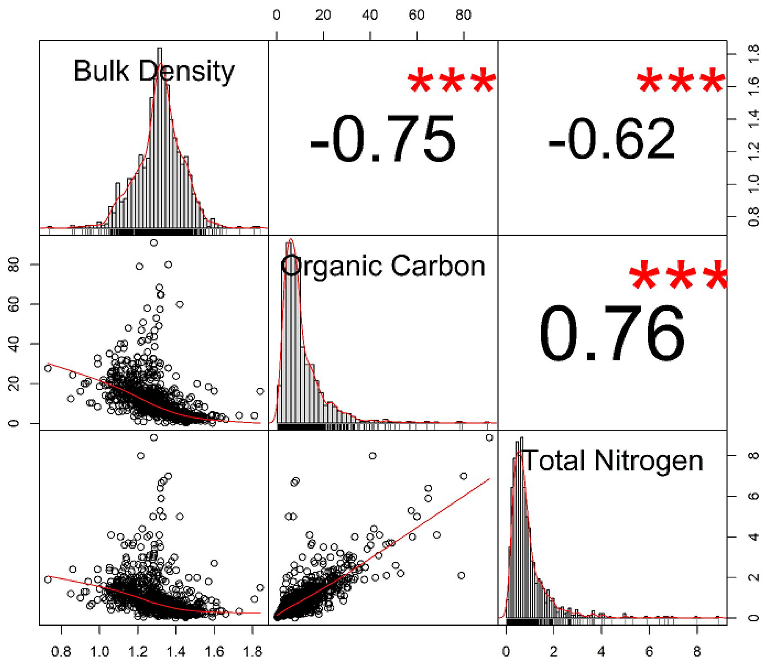
| Bulk Density (g/cm3) | Organic Carbon (g/kg) | Total Nitrogen (g/kg) | |
|---|---|---|---|
| Average | 1.31 | 10.52 | 0.92 |
| Standard deviation | 0.12 | 9.45 | 0.88 |
| Sample variance | 0.01 | 89.32 | 0.77 |
| Coefficient of variation (%) | 9.10 | 89.44 | 95.65 |
| Minimum | 0.73 | 0.20 | 0.01 |
| Maximum | 1.84 | 91.00 | 8.90 |
© 2020 by the author. Licensee MDPI, Basel, Switzerland. This article is an open access article distributed under the terms and conditions of the Creative Commons Attribution (CC BY) license (http://creativecommons.org/licenses/by/4.0/).
Share and Cite
Boluwade, A. Joint Simulation of Spatially Correlated Soil Health Indicators, Using Independent Component Analysis and Minimum/Maximum Autocorrelation Factors. ISPRS Int. J. Geo-Inf. 2020, 9, 30. https://doi.org/10.3390/ijgi9010030
Boluwade A. Joint Simulation of Spatially Correlated Soil Health Indicators, Using Independent Component Analysis and Minimum/Maximum Autocorrelation Factors. ISPRS International Journal of Geo-Information. 2020; 9(1):30. https://doi.org/10.3390/ijgi9010030
Chicago/Turabian StyleBoluwade, Alaba. 2020. "Joint Simulation of Spatially Correlated Soil Health Indicators, Using Independent Component Analysis and Minimum/Maximum Autocorrelation Factors" ISPRS International Journal of Geo-Information 9, no. 1: 30. https://doi.org/10.3390/ijgi9010030
APA StyleBoluwade, A. (2020). Joint Simulation of Spatially Correlated Soil Health Indicators, Using Independent Component Analysis and Minimum/Maximum Autocorrelation Factors. ISPRS International Journal of Geo-Information, 9(1), 30. https://doi.org/10.3390/ijgi9010030