Extracting Building Areas from Photogrammetric DSM and DOM by Automatically Selecting Training Samples from Historical DLG Data

Abstract

This paper presents an automatic building extraction method which utilizes a photogrammetric digital surface model (DSM) and digital orthophoto map (DOM) with the help of historical digital line graphic (DLG) data. To reduce the need for manual labeling, the initial labels were automatically obtained from historical DLGs. Nonetheless, a proportion of these labels are incorrect due to changes (e.g., new constructions, demolished buildings). To select clean samples, an iterative method using random forest (RF) classifier was proposed in order to remove some possible incorrect labels. To get effective features, deep features extracted from normalized DSM (nDSM) and DOM using the pre-trained fully convolutional networks (FCN) were combined. To control the computation cost and alleviate the burden of redundancy, the principal component analysis (PCA) algorithm was applied to reduce the feature dimensions. Three data sets in two areas were employed with evaluation in two aspects. In these data sets, three DLGs with 15%, 65%, and 25% of noise were applied. The results demonstrate the proposed method could effectively select clean samples, and maintain acceptable quality of extracted results in both pixel-based and object-based evaluations.

1. Introduction

With the ongoing urbanization and city expansion worldwide, many international cities are experiencing rising construction activities. In addition, many cities in China are expressing the need to construct smart cities, hence the intelligent understanding of geographical information from different sensors (e.g., remote sensed images, laser scanning point clouds) becomes a necessity for city management departments. Building extraction serves an important role and it is also the basis for building change detection, three-dimensional (3D) building modeling, and further urban planning.

Building extraction is a popular research topic in the field of photogrammetry and computer vision. Automatic building extraction methods have become a hot research topic for scholars worldwide. A great variety of methods have been proposed, and they can be generally classified into two categories: unsupervised methods and supervised methods.

The first category (unsupervised methods) is mainly developed with some weak prior knowledge or basic assumptions. For example, Du et al. introduced a graph cuts-based method and applied it in light detection and ranging data (LiDAR) [1]. Its energy function is constructed by some hand-crafted features which obviously might not satisfy all kinds of situations in complicated urban scenes. Huang et al. stated a concept called ‘morphological building index’ (MBI) to extract buildings in high-resolution images [2]. This index mainly concerns the relationship between the spectral-structural characteristics of buildings and the morphological operators. However, this kind of relationship cannot sufficiently represent all kinds of remote sensed images. Since vegetation is hard to distinguish from buildings, some methods were designed to filter vegetation area and then apply some morphological operations [3,4,5]. According to some studies [3,4], the application of a normalized difference vegetation index (NDVI) is helpful for filtering of vegetation areas and obtaining better extraction results. Nevertheless, the NDVI is not applicable in RGB (red, green, blue) images. Whilst some color vegetation index methods were developed to tackle this problem [6], these methods contain some limitations and are difficult to apply elsewhere. In all, unsupervised methods are developed based on some poor prior knowledge which can satisfy a certain kind of situation or urban scene. Suppose the constructions in cities become more complicated, these methods would then show their shortcomings.

The second category (supervised method) can achieve more satisfying results especially along with deep learning methods [7]. To obtain satisfying results, adequate training samples are needed. It is well known that training samples labeling is a time-consuming task. To reduce the need for manual labeling, several methods introduce existing geographical information system (GIS) data or open source data to acquire training labels automatically [8,9]. However, existing GIS data like historical digital line graph (DLG) data may contain noise for the change of buildings in time gap. Volunteered geographical information (VGI) like OpenStreetMap (OSM) data may include position error and attribute error. The former is mainly caused by the inconsistency between OSM data and remote sensed data, while the latter is primarily driven by incorrect labels provided by amateurish volunteers [10]. To handle this problem, several methods for selecting clean parts in noisy labels were proposed. In an earlier study [11], an overview towards classification with noisy labels concludes three main strategies to address this issue. In a study by Wan et al. [10], for example, a fuzzy c-means (FCM) method was applied to avoid possible error caused by OSM data, and cluster each class of possible training samples. In other studies [8,12], iterative training in random forest (RF) classifier was adopted to select clean samples, because RF classifier has proven to be robust to label noise.

Other than sample label, feature is another key affecting the final classification result. It is common for people to design features in accordance to some prior knowledge from simple observation or basic assumptions. For example, some kinds of hand-crafted features are designed (e.g., contextual features, spatial features, and spectral features) [1,13,14,15]. As mentioned above, hand-crafted features designed by humans have some limitations. They cannot cover enough situations in more complicated urban scenes nowadays and produce unpromising results. In recent years, deep learning has been introduced to the field of remote sensing image semantic segmentation and classification [16,17]. However, training a deep network from scratch for a remote sensing task needs a lot of related samples. Thus, transfer learning via deep learning was proposed to lessen the overdependence on the training sample [18]. To maintain the diversity of features, spectral information and height information should be both treated as the input data of transfer learning.

Among these methods, the building extraction results based on LiDAR data or a combination of remote sensed images and LiDAR data are better than only applying images. This is because LiDAR data can provide useful information that supports building extraction [19,20,21], including accurate 3D coordinates, context information, and spectral information. Unfortunately, these methods cannot be widely applied in many cities, because LiDAR data is expensive and not always available. To address this issue, some scholars have tried to use dense image matching (DIM) point cloud data to substitute LiDAR data. Along with the development of multi-view system (MVS) technology and the aerial oblique image system, the digital surface model (DSM) can be easily obtained, which provides an alternative data source of height information.

The contributions of this paper can be concluded as two aspects mainly. Firstly, to reduce manual labeling, historical DLG data is applied to obtain enough training labels automatically. As historical DLGs update frequently in cities, the noise should maintain at a certain level. An iterative method is used to remove possible errors in the initial label. Secondly, to obtain effective features, deep features extracted from spectral information derived from a digital orthophoto map (DOM) and height information derived from DSM by a pre-trained fully connected network (FCN) are combined. In this paper, the deep features are extracted in pixel-wise. To ensure the efficiency of the iterative processing and avoid potential harm brought by high feature dimension, the principle component analysis (PCA) algorithm is applied to reduce the dimensions of deep features.

The rest of this paper is organized as follows: the proposed methodology is described in detail in Section 2. The experimental data sets and related evaluation criteria are introduced in Section 3. The correspondent results and discussion from four aspects are shown in Section 4. And finally, the conclusion and future work are presented in Section 5.

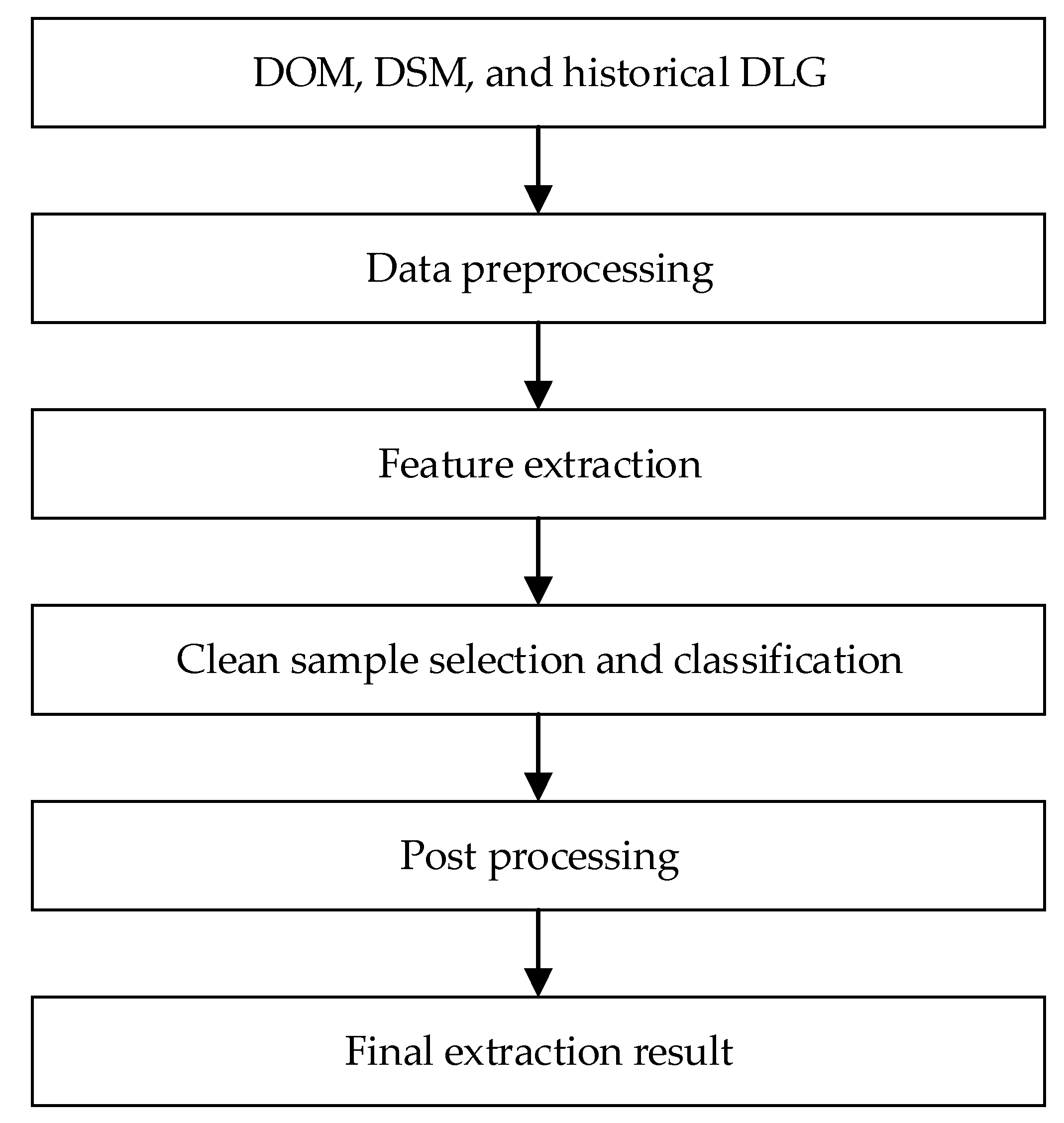
2. Methods

2.1. Overview the Method

The general workflow of our proposed method is shown in Figure 1. It consists of four main steps: data preprocessing, feature extraction, clean sample selection and classification, and post processing. Full descriptions of each step will be explained in the following subsections.

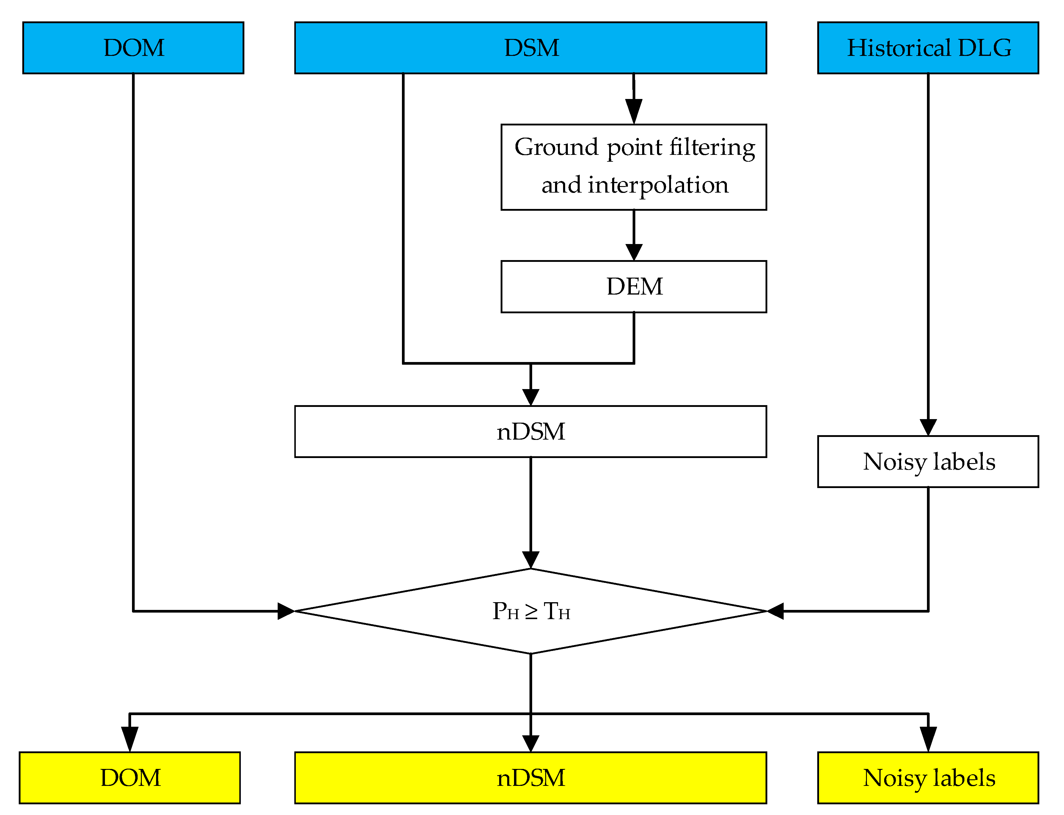
2.2. Data Preprocessing

The workflow of preprocessing is shown in Figure 2 (where the input data is marked in blue and the output result is marked in yellow). The DSM, DOM, and the corresponding DLG are all aligned well and their sizes are all the same. Firstly, the DSM is filtered to ground points and non-ground points by using the cloth simulation filter (CSF) [22] implemented in CloudCompare [23]. Then these ground points are used to interpolate the digital elevation model (DEM) by means of the Kriging method. Finally, DEM is subtracted from the DSM to produce the normalized DSM (nDSM) image which represents the actual heights of objects. In this paper, the nDSM image is a three-channel image which satisfies the requirement for later feature extraction. For each pixel in the nDSM image, the values in three channels are identical.

The newly obtained DSM and DOM are registered well with historical DLG data. The DLG data can be used to support the building area extraction on the newly obtained data. Nevertheless, with frequent changes in modern cities, some buildings in the DLG data might be demolished in the newly obtained DSM and DOM, while other buildings might appear in the newly obtained DSM and DOM. In this case, the building area derived from DLG includes a certain degree of noise.

As the DEM is obtained, the building area extraction task can be simplified to distinguish the building from other objects above ground. Thus, a non-building area mask is generated based on the nDSM and is used to identify some pixels belonging to the non-building area directly. It comes with a simple assumption that the height of buildings should be higher than a threshold $T_H$ in urban scenes. As shown in Figure 2, we express this assumption by the height of current pixel $P_H$ which is no less than a given threshold $T_H$ ($P_H\ge T_H)$. The value of $T_H$ should be set according to situations in different urban areas. After deriving the non-building mask, it is applied to retain pixels of the DOM, nDSM, and initial labels only in the possible building area (the yellow items in Figure 2) for subsequent processing.

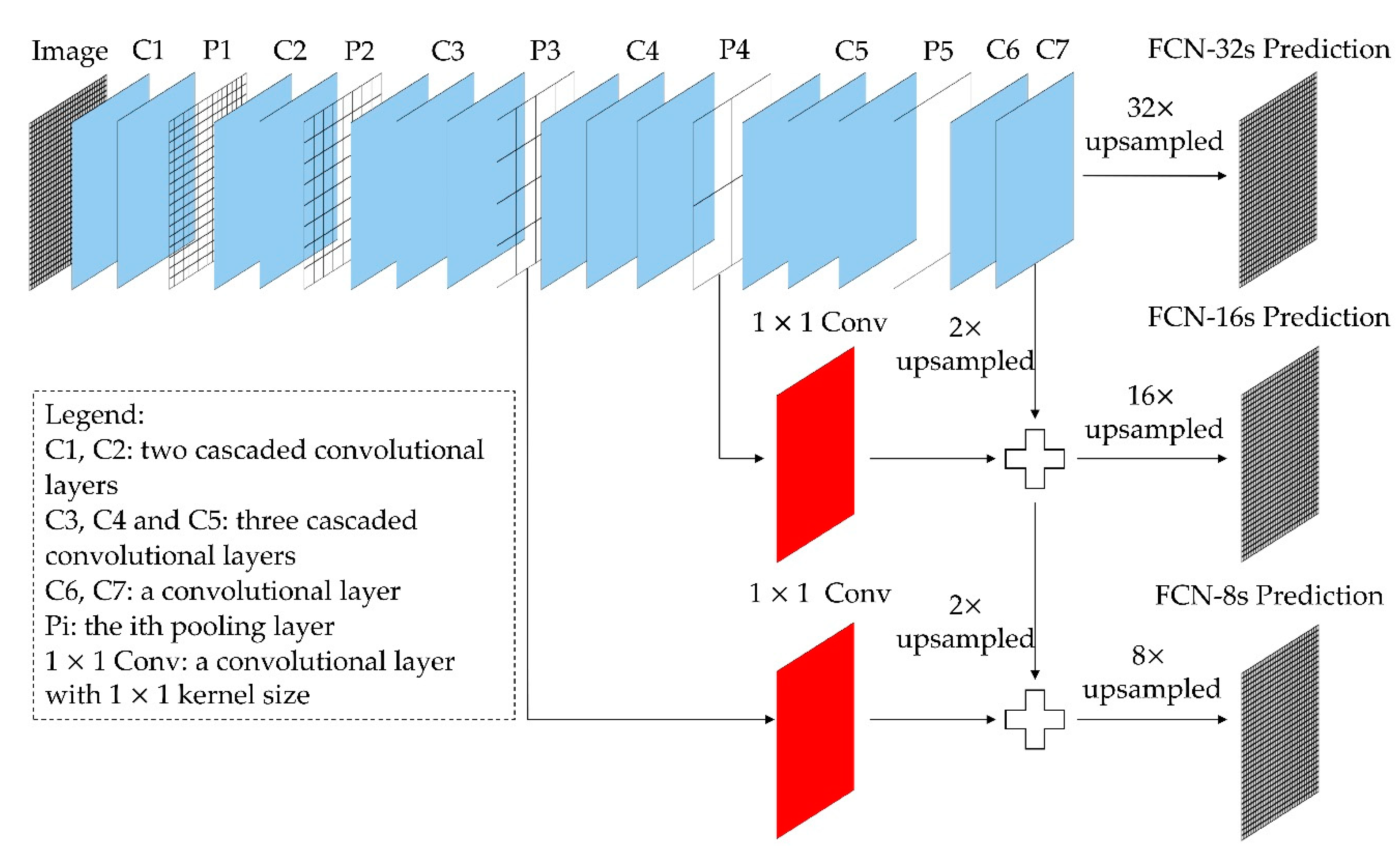
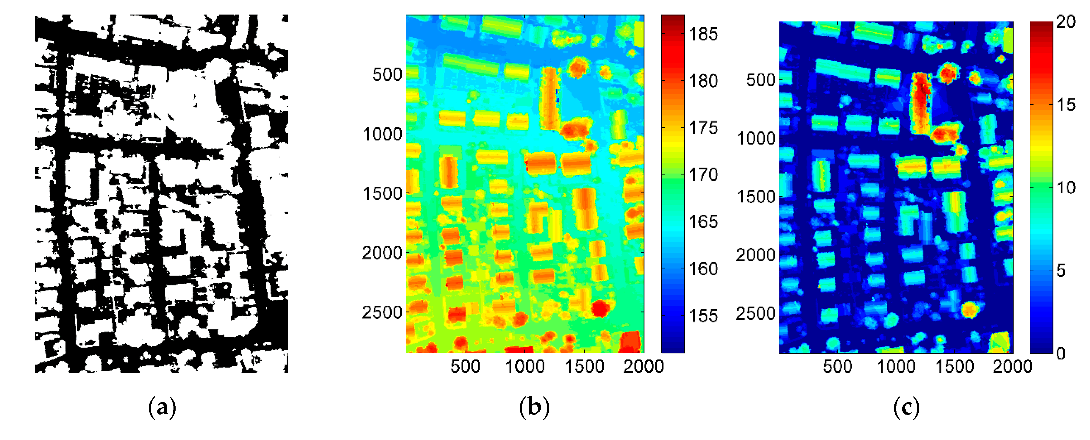
2.3. Feature Extraction

In this paper, deep features are extracted in pixel-wise of both the DOM image and nDSM image. FCNs can accept images without size restriction and produce 2D spatial outputs with corresponding size, which secure the spatial information in input images against lost or change [24]. FCN-8s pre-trained on PASCAL VOC dataset for semantic object segmentation was adopted to extract deep features in this paper [25]. The structure of the employed FCN is displayed in Figure 3.

Considering both height information and spectral information, a forward computation of FCN-8s is directly carried out on both the DOM image and nDSM image to extract deep features. Then, the feature map from the first convolutional layer after P1 is adopted, because it is more likely to respond to the edge of the object. After that, a bilinear up-sampling processing is performed to derive a 128-d (128 dimensions) feature vector for each pixel of the input image. In the proposed method, the DOM image and nDSM image are used to extract 128-d deep features by FCN-8s separately.

To control the computation cost and avoid the potential harm brought by the high dimensions of the obtained features, the PCA algorithm is used to reduce the feature dimensions and alleviate the feature redundancy [26]. The deep feature dimensions of nDSM and DOM are empirically reduced to 7-d (7 dimensions) and 12-d (12 dimensions), respectively.

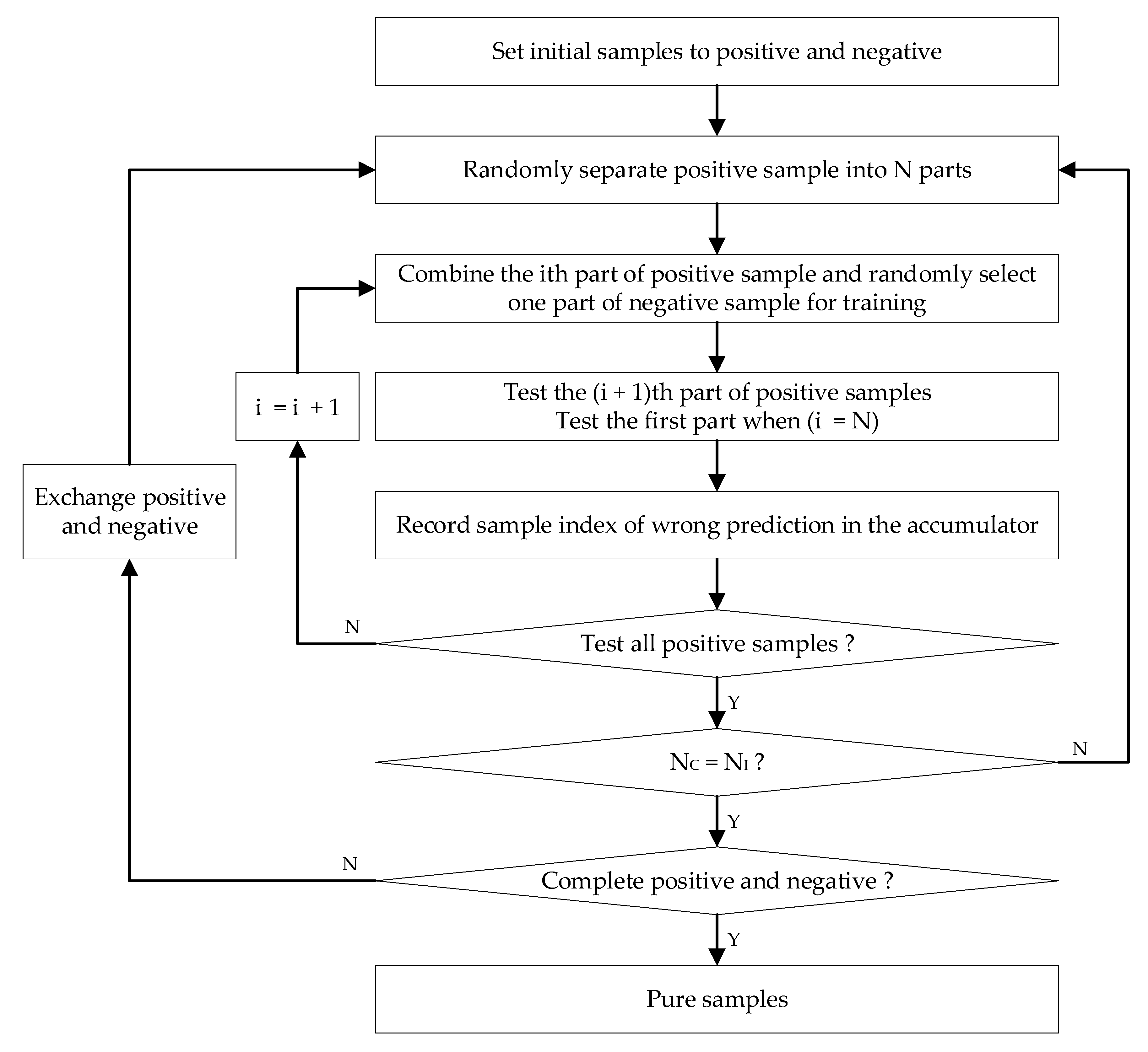
2.4. Clean Sample Selection and Classification

To purify the noise labels obtained in the preprocessing step, an iterative method inspired by the works in [8,12] was proposed. The workflow is presented in Figure 4. It starts from the initial noisy labels from the data preprocessing step. The iterative processing performs as a leave-one-out cross-validation approach. It can be supposed that the trained classifier based on the initial labels performs better than a random guess, so those incorrect samples would likely be predicted with labels different from the given labels. By randomly segmenting the training samples and the testing samples, each iteration can be regarded as independent testing. So, a sample is more likely to be clean when its initial label agrees more times with the predicted result.

At the beginning, pixels labeled as ‘building’ are considered positive samples, and pixels labeled as ‘non-building’ are considered negative samples. To balance the amount of positive and negative samples, both samples are divided into several parts. If we set the number of positive samples to $N_P$, and set the number of negative samples to $N_N$, the ratio of $N_P$ and $N_N$ is calculated using Equation (1). If $N_P$ and $N_N$ differ obviously ($\mathrm{ratio}\ge 2$), the positive samples are divided into $\mathrm{N}$ parts and the negative samples are divided into $\mathrm{M}$ parts ($\mathrm{N}\ne \mathrm{M}$). In each part of the positive samples or negative samples, the number of samples is the greatest common divisor of $N_P$ and $N_N$. If the $\mathrm{ratio}<2$, both the positive samples and negative samples are separated into two parts ($\mathrm{N},\mathrm{M}=2$) so that the number of positive samples and negative samples are approximately equal.

$$\mathrm{ratio}=\frac{Max\left(N_P, N_N\right)}{Min\left(N_P, N_N\right)}$$

(1)

After that, clean samples are selected in two steps. The positive side is processed at first. The ${\mathrm{i}}_{th}$ part of positive samples $(P_i,$ $\mathrm{i}$ = $1:\mathrm{N})$ and one randomly selected part from the negative samples are combined to train a RF classifier, and then test the ${(\mathrm{i}+1)}_{th}$ part of positive samples $\left(P_{i+1}\right).$ Specifically, when it turns to the ${\mathrm{N}}_{th}$ part of the positive samples $(P_N),$ the first part of positive samples $\left(P_1\right)$ is tested. After training $\mathrm{N}$ times, all positive samples are tested once and the first iteration is completed. After iterating $N_I$ times, the positive side is finished. This is followed by the negative side. Similar methods are applied and the difference is training for $\mathrm{M}$ times in one iteration. In the former process, an accumulator, regarded as ACC hereafter, is initialized into zero at the beginning. If some samples are wrongly predicted in each iteration, an ACC would add one in the corresponding position. After processing both sides, ACC is used to determine whether a sample is correct or not. Following Equation (2), if the ratio of wrongly predicting times is less than ${\theta }_T,$ the corresponding pixel will be taken as a right labeled sample, then the label L(P) is set to 1 which stands for a clean sample. Otherwise, it will be set to 0 which stands for an impure sample.

$$\mathrm{L}\left(\mathrm{P}\right)=\{\begin{array}{c}1 \left(stands for pure sample\right), if \frac{N_W}{N_I}<{\theta }_T\\ 0 \left(stands for impure samples\right), if \frac{N_W}{N_I}\ge {\theta }_T\end{array}$$

(2)

where $N_W$ is the number recorded in the ACC.

Based on the selected clean samples, a final RF classifier is trained to predict the remaining confused samples to gain the initial building area extraction result.

2.5. Post Processing

Since the initial result is obtained in pixel-wise, some pixels could be wrongly predicted (e.g., building area predicted as non-building area, and non-building area predicted as building area). To make the results more reasonable, two methods are adopted for post processing: connected component analysis (CCA) and the close operation in morphological processing. Since a building will occupy an area on the nDSM, a CCA operation is performed on the initial classification result. Then, some connected components with less than a given threshold $T_S$ are removed from the building extraction result. This process can remove some errors presented in the form of salt noise. The close operation is mainly used to fill empty holes in a connected area to ensure the completeness of the building extraction result. The refined results are treated as final extraction results of the proposed method.

3. Data Sets and Evaluation Criteria

The proposed method was implemented using Python language, except the ground points filtering in the pre-processing step was carried out using CloudCompare. A desktop computer with Inter Core i7-8700 CPU at 3.19 GHz was used to perform the experiments.

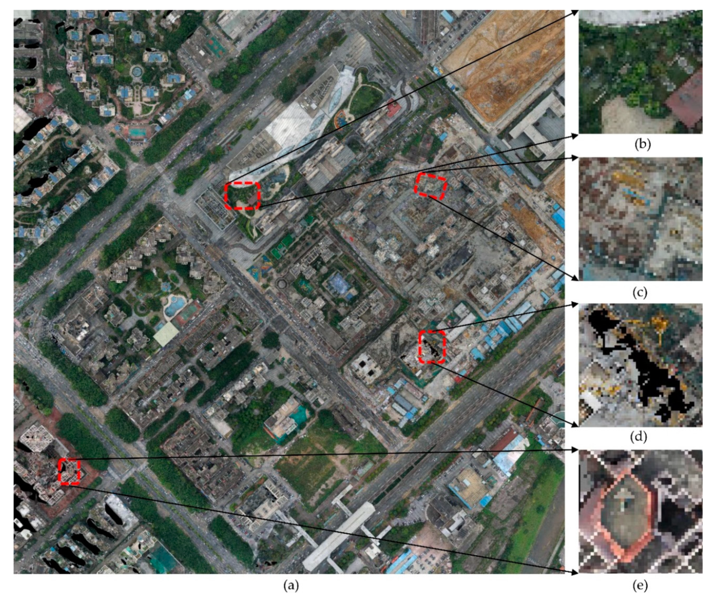
3.1. Data Sets Description

To evaluate the proposed method, data sets covering two different areas were employed. Figure 5 illustrates the data of the first area provided by ISPRS Test Project on Urban Classification and 3D Building Reconstruction, which is located in the city of Vaihingen, Germany. It is regarded as Area1 hereafter. The ground truth of the building map was manually edited to simulate the historical DLG (represented using DLG_M hereafter; Figure 5a). The spatial resolutions of DOM, DSM, and DLG_M were all 0.09 m, and the sizes of these data were 2002 × 2842 pixels. The DOM is a pan-sharpened color infrared (CIR) image. To show more details of the first data set, the three images were clockwise rotated, as represented in Figure 5c.

The data sets covering the second area, located in the city of Shenzhen, China, are shown in Figure 6 and Figure 7. Compared to Area1, there are many buildings under construction in Shenzhen and the building shapes are somewhat irregular. It is regarded as Area2 hereafter. The photogrammetric DOM and DSM were derived from airborne oblique images obtained in 2016 and generated using ContextCapture and the resolution was downsampled to 0.5 m. The first historical DLG data were acquired in 2008 (Figure 6a), and the second historical DLG data were obtained in 2014 (Figure 7a). Since the two historical DLGs were provided in the form of a vector, they were transferred to raster images to match the spatial resolution of the DOM and DSM. After unifying the resolution, the raster images derived from DLGs were cropped to the same size of the DSM and DOM. The size was 1503 × 1539 pixels. The cropped raster image derived from the DLG (obtained in 2008) is represented using DLG2008 hereafter, while the other derived image is represented using DLG2014.

To clearly illustrate the experiment data, the original DLG was superposed on the nDSM with blue boundaries as shown in Figure 5c, Figure 6c, and Figure 7c. The noise level of DLG_M, DLG2008, and DLG2014 was about 15%, 65%, and 25%, respectively. From the illustration, it can be seen that the change ratio between DLG2008 and the new DSM was very obvious compared to the ratio between the DLG2014 and the new DSM. Due to the long time lapse, it is difficult to automatically select samples from DLG data.

3.2. Assessment Criteria

Three criteria proposed in [27] were adopted for quantity evaluation of the results. They are defined as Equations (3)–(5):

$$\mathrm{Completness}=\frac{TP}{\left(TP+FN\right)}$$

(3)

$$\mathrm{Correctness}=\frac{TP}{\left(TP+FP\right)}$$

(4)

$$\mathrm{Quality}=\frac{TP}{\left(TP+FN+FP\right)}$$

(5)

where TP, FN, and FP mean true positive, false negative, and false positive, respectively. Here, TP stands for the building area being detected as a building area, FN stands for the building area being detected as a non-building area, and FP stands for a non-building area being detected as a building area. In the following sections, all the extraction results are assessed by these three criteria in both pixel-based aspect and object-based aspect. Suppose at least 50% of a building is detected, this building is considered to be correctly classified in object-based assessment.

3.3. Parameters Setting

The height threshold $T_H$ of Area1 and Area2 are empirically set to 1 m and to 3 m, respectively. The number of iterations $N_I$ is empirically set to 10, and the tolerance rate ${\theta }_T$ is empirically set to 0.1. This means only pixels which are not be predicted wrong each time ($N_W=0$) are treated as clean samples. The area threshold $T_S$ of Area1 and Area2 are set empirically to 10 m² and 25 m², respectively.

4. Results and Discussion

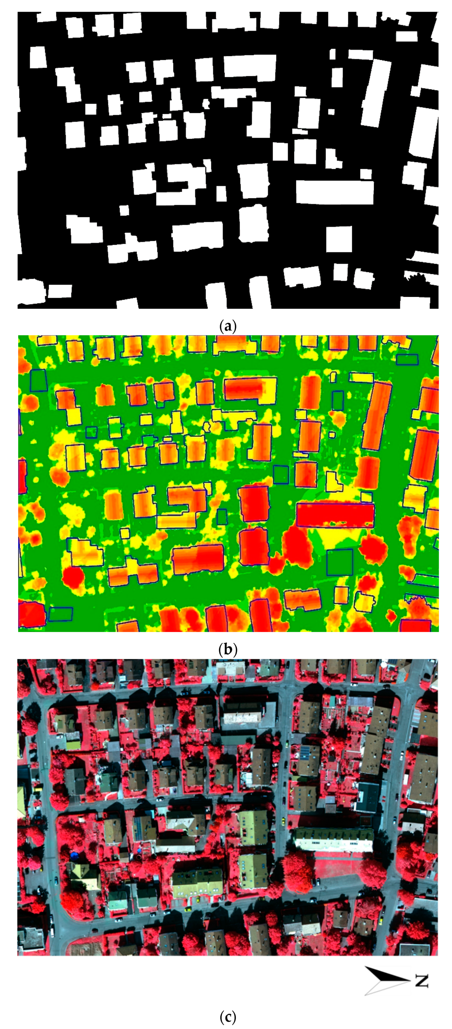
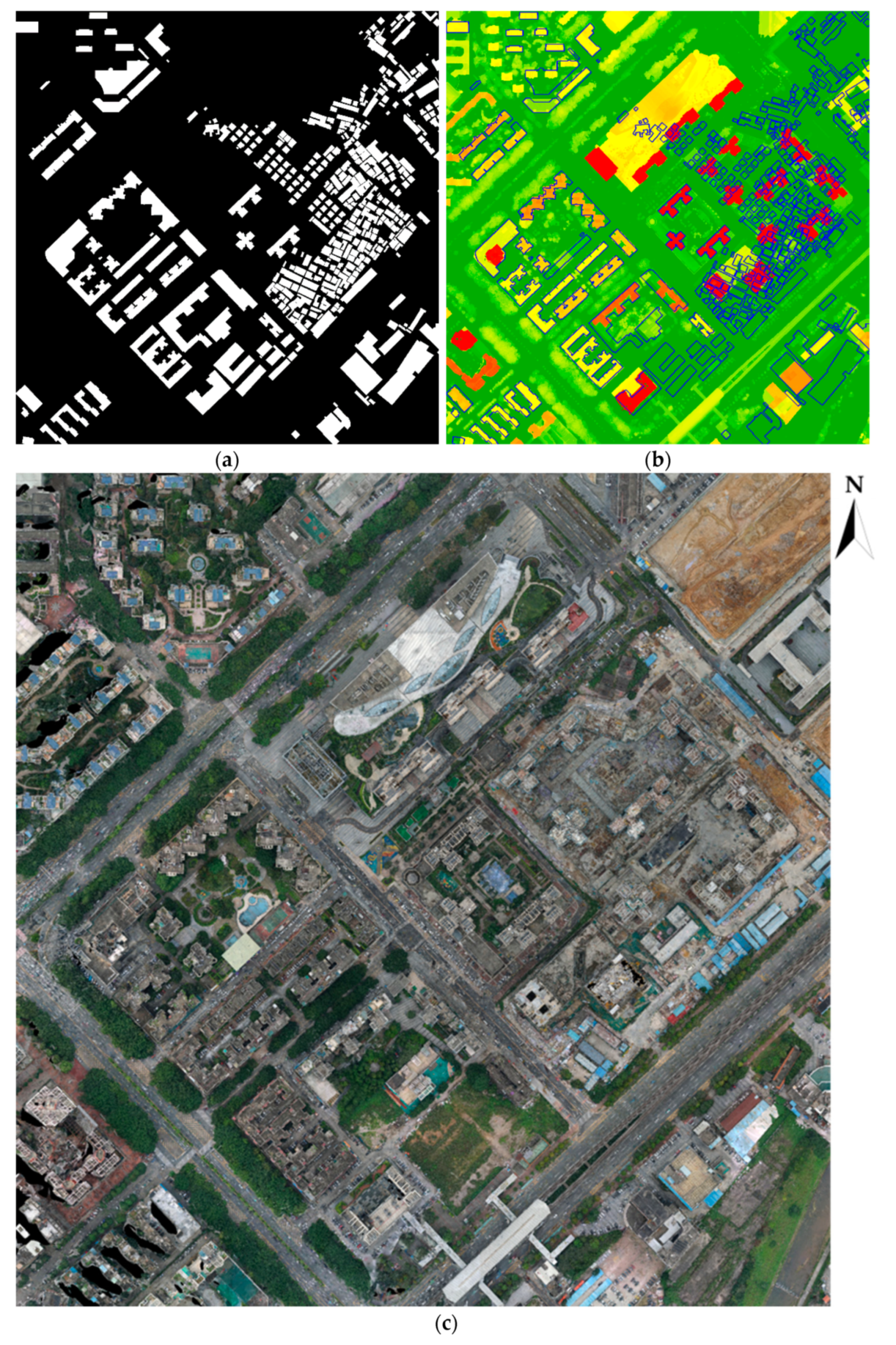
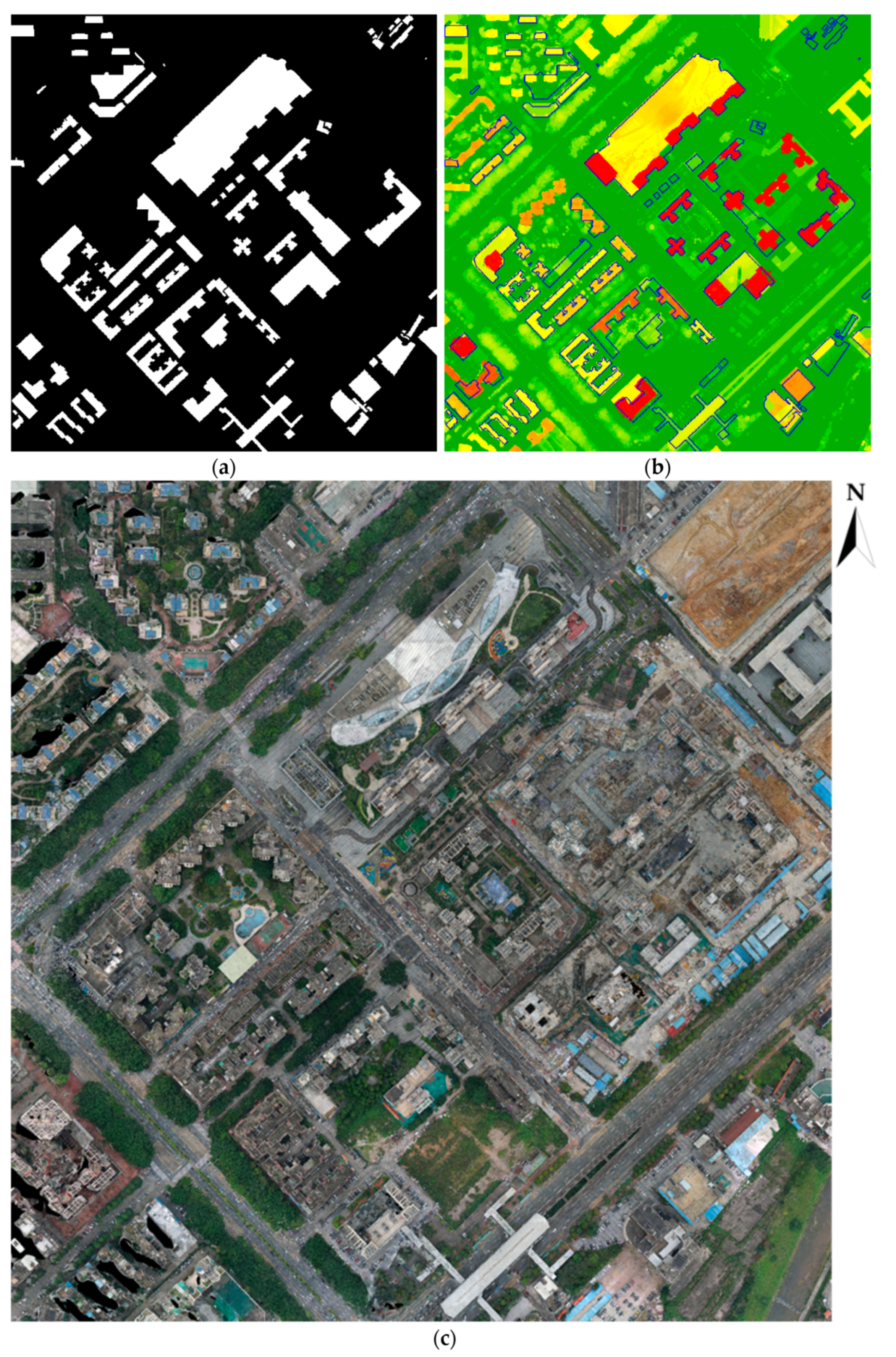
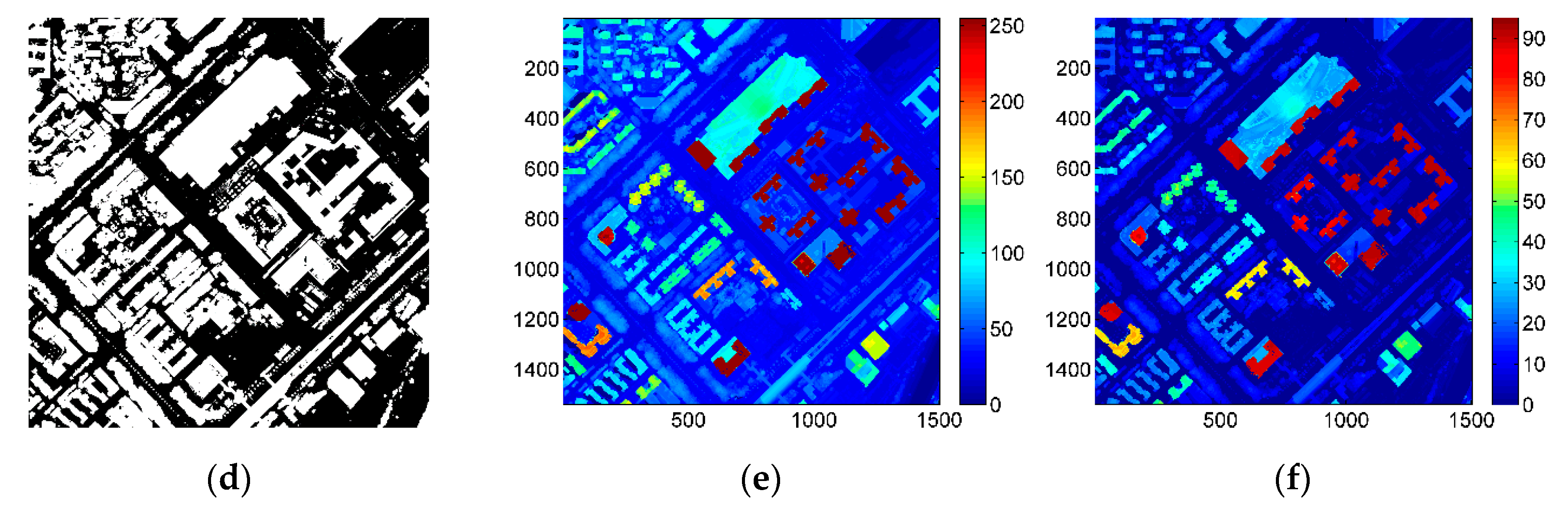
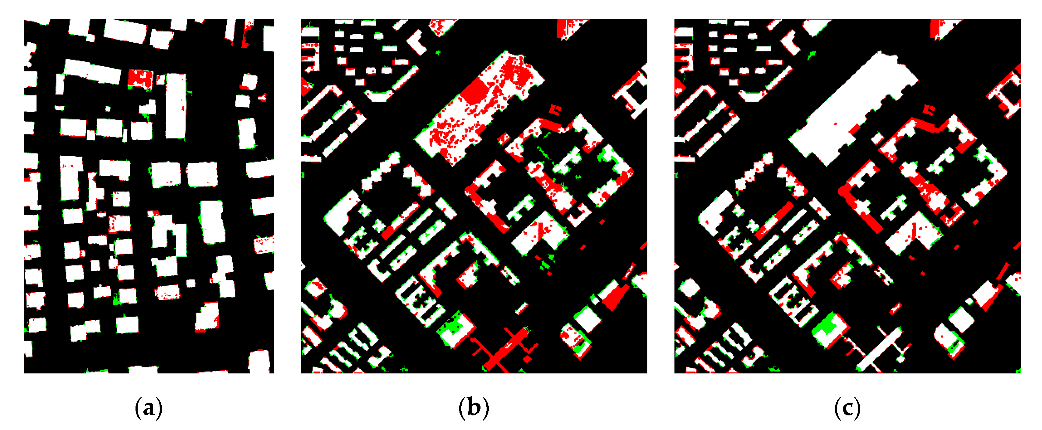
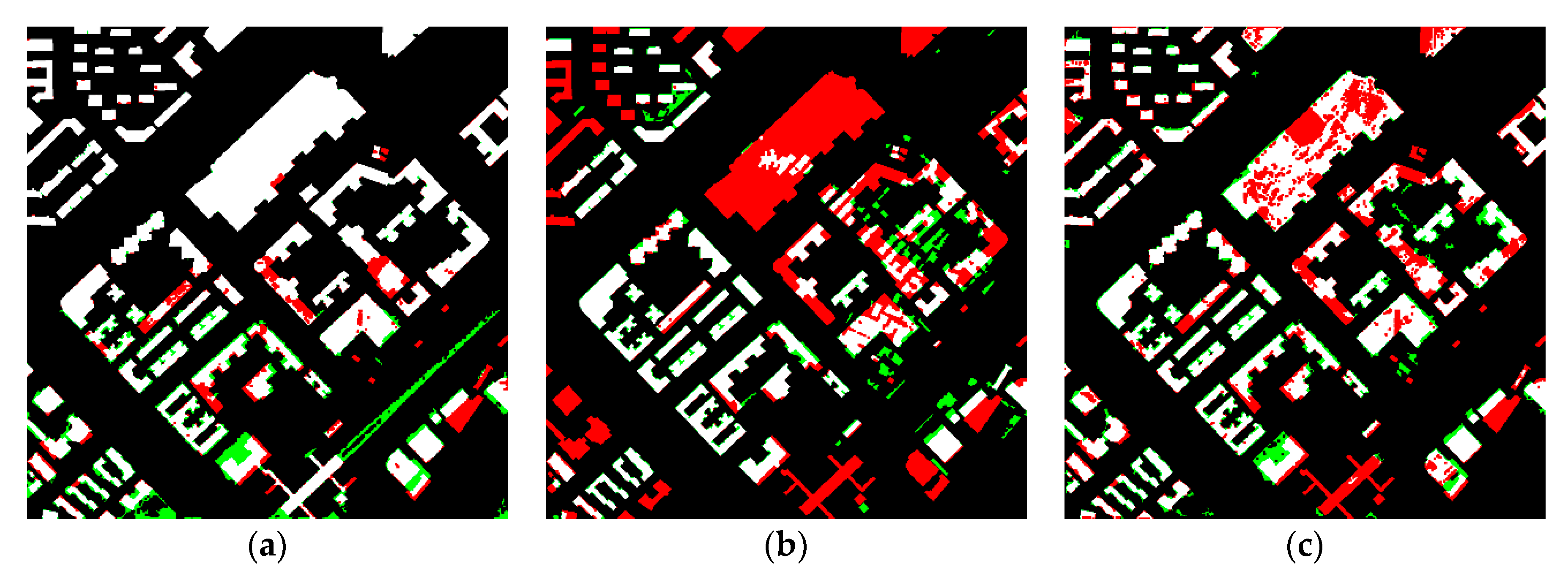
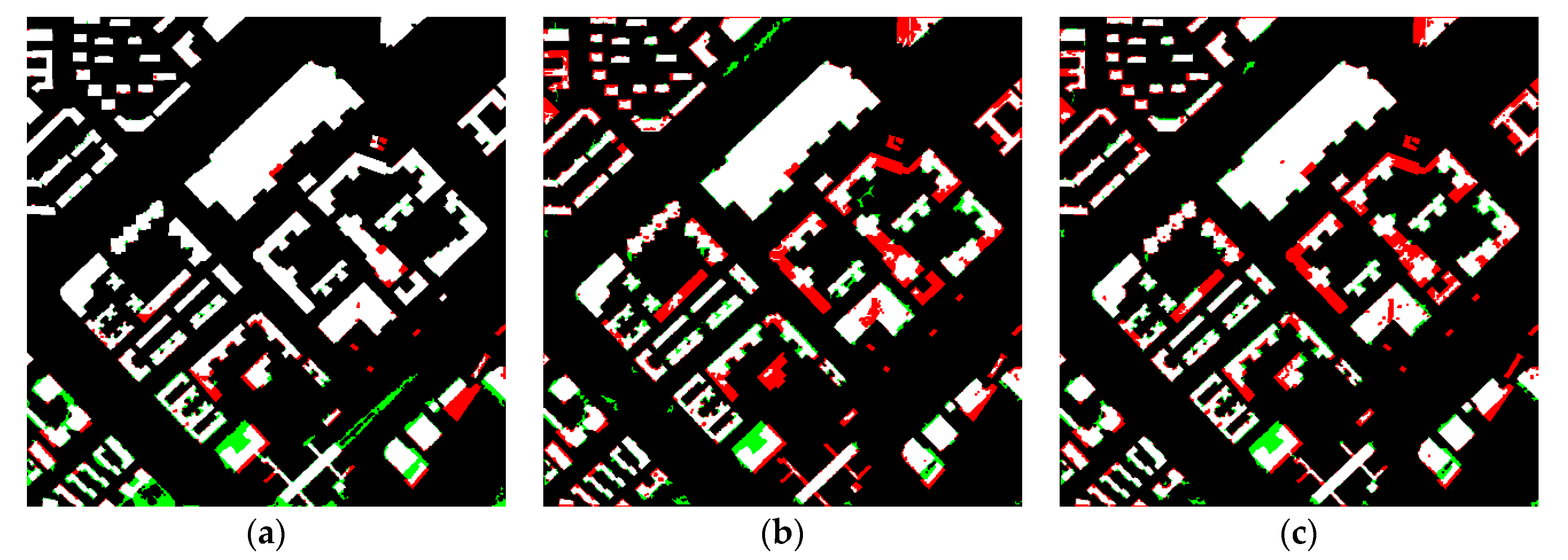
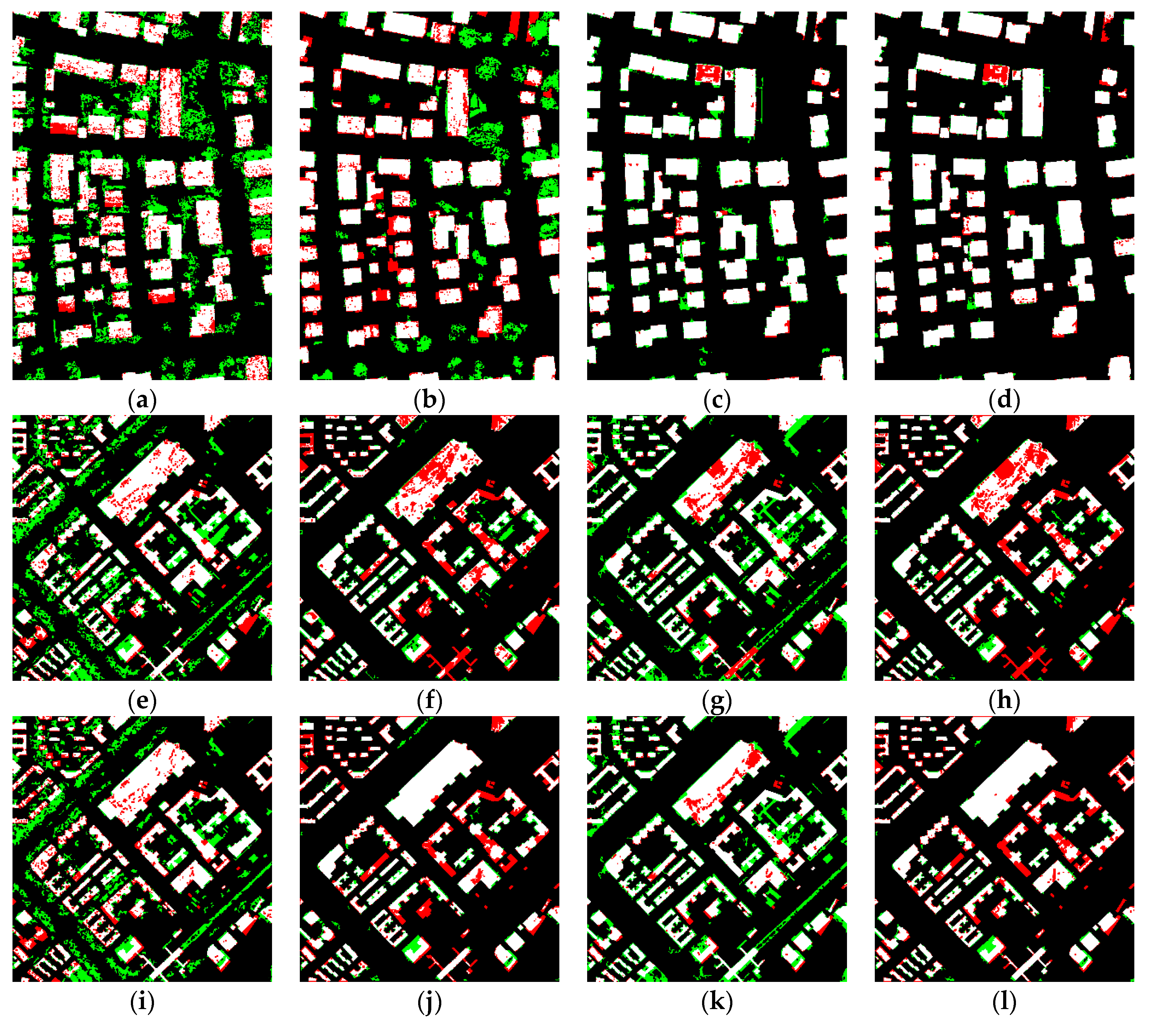
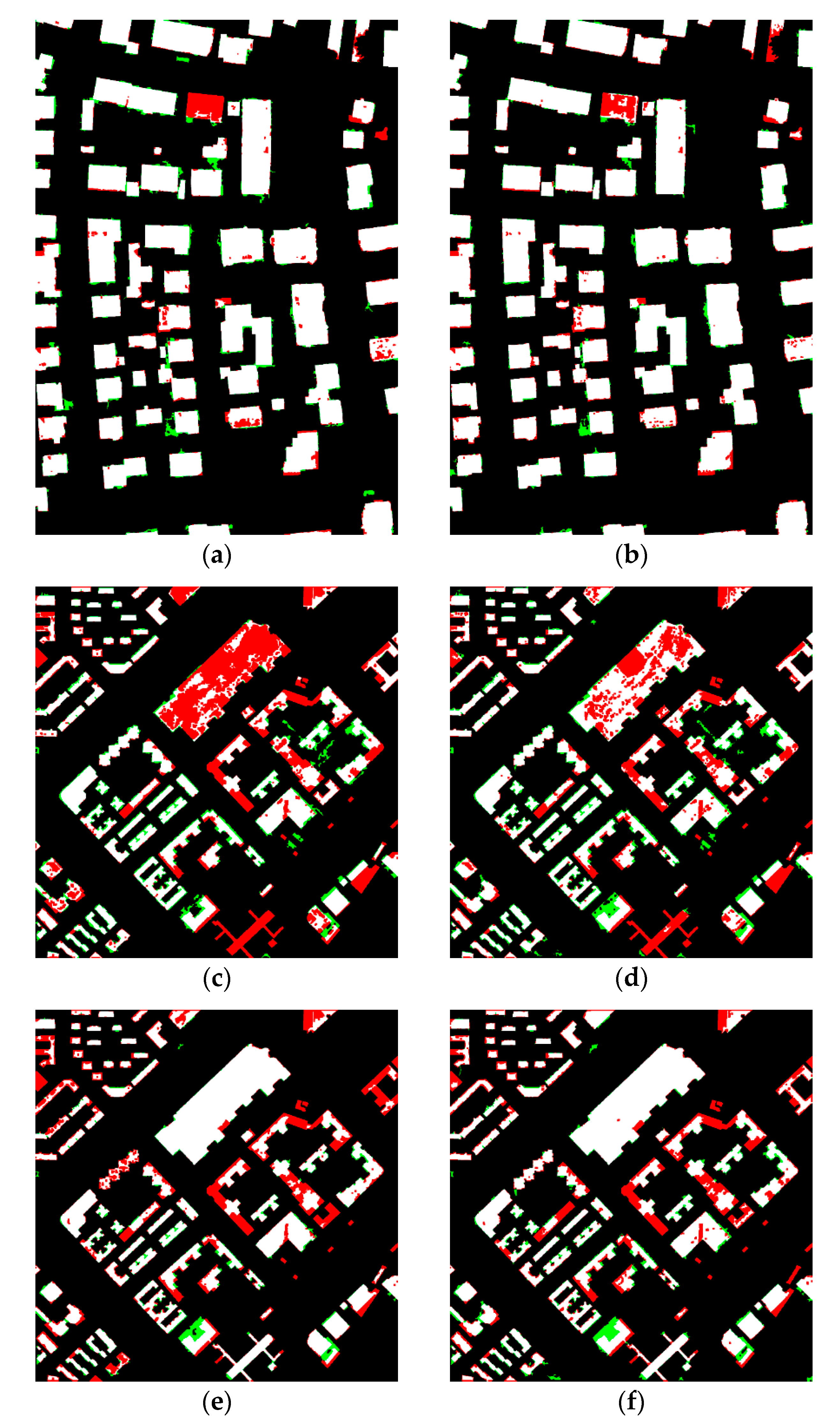
4.1. Results

The data pre-processing results are presented in Figure 8. The building extraction results are presented in Figure 9. The corresponding accuracy assessment results are presented in

Table 1. The accuracy assessments of three results.

Data Sets		Pixel-Based (%)			Object-Based (%)
		Completeness	Correctness	Quality	Completeness	Correctness	Quality
Area1	DLG_M	93.22	96.52	90.19	97.33	94.81	92.41
Area2	DLG2008	70.05	87.07	63.45	87.91	87.91	78.43
	DLG2014	77.52	92.33	72.83	86.81	92.94	81.44

. In Figure 8a,d, the black parts stand for non-building areas, while the white parts stand for the possible building areas taking part in clean sample selection. Moreover, different contrast effects between DSM and nDSM are visible. The former (Figure 8b,e) considers the height of the terrain, while the latter describes the actual heights of objects in urban scenes (Figure 8c,f). In the following figures representing building extraction results, the white stands for correctly classified (TP), the red stand for missing classification (FN), and the green stands for wrongly classified (FP).

Table 1 presents the accuracy assessments of building extraction results in three data sets. The evaluations of all items are above 90% in Area1 with DLG_M. In Area2 with DLG2008, the correctness in both pixel and object aspects reaches 87%, while the pixel-based evaluation of completeness is about 70%. When it turns to DLG2014 in Area2, the evaluation of correctness in both pixel and object aspects exceeds 92%, but the pixel-wise evaluation of completeness is below 80%. In general, it is easy to achieve above 90% of quality in Area1 with DLG of 15% noise. In Area2, 78% of quality evaluation in the object aspect is obtained when applying DLG of 65% noise, while the object-based quality evaluation can hit 81% when using 25% noise DLG.

4.2. Discussion

4.2.1. Label Selection

Three strategies concerning label selection were compared and analyzed: (1) using ground truth data as labels; (2) using historical DLG data as labels; and (3) using selected labels from clean samples (proposed). In this paper, a certain number of samples can be selected and treated as clean. The same number of ground truth data is also randomly selected to complete strategy (1) to evaluate our method more reasonably. In

Table 2. The accuracy assessment of three strategies in Area1 with DLG_M.

Strategy	Pixel-Based (%)			Object-Based (%)
	Completeness	Correctness	Quality	Completeness	Correctness	Quality
(1)	98.45	99.53	97.99	100.00	98.68	98.68
(2)	89.53	99.76	89.34	89.33	98.53	88.16
(3)	93.22	96.52	90.19	97.33	94.81	92.41

,

Table 3. The accuracy assessment of three strategies in Area2 with DLG2008.

Strategy	Pixel-Based (%)			Object-Based (%)
	Completeness	Correctness	Quality	Completeness	Correctness	Quality
(1)	89.77	89.10	80.89	90.10	92.13	83.67
(2)	47.52	82.44	43.15	47.25	50.00	32.09
(3)	70.05	87.07	63.45	87.91	87.91	78.43

and

Table 4. The accuracy assessment of three strategies in Area2 with DLG2014.

Strategy	Pixel-Based (%)			Object-Based (%)
	Completeness	Correctness	Quality	Completeness	Correctness	Quality
(1)	93.17	92.15	86.32	93.41	91.40	85.86
(2)	73.33	97.61	72.03	64.84	83.10	57.28
(3)	77.52	92.33	72.83	86.81	92.94	81.44

, these three strategies are represented as strategy (1), (2), and (3), respectively. If the selected samples are clean enough, the accuracy assessment of results by strategy (3) should be between the corresponding assessment of strategy (1) and strategy (2).

Figure 10 shows the results of three strategies in Area1 with DLG_M, and Table 2 displays the corresponding accuracy assessments. Note that in strategy (1), 261,8281 samples were randomly selected (3,047,394 samples in total, about 86% of samples were selected) from ground truth data, and the same number of clean samples from DLG_M was selected in strategy (3).

Figure 11 shows the results of three strategies in Area2 with DLG2008, and Table 3 presents the corresponding accuracy assessments. Note that in strategy (1), 555,318 samples were randomly selected (1,056,178 samples in total, about 52% of samples were selected) from ground truth data, and the same number of clean samples from DLG2008 was selected in strategy (3).

Figure 12 shows the results of three strategies in Area2 with DLG2014, and Table 4 shows the corresponding accuracy assessments. Note that in strategy (1), 732,214 samples were randomly selected (1,056,178 samples in total, about 69% of samples were selected) from ground truth data, and the same number of clean samples from DLG2014 was selected in strategy (3).

In general, the figures (Figure 10, Figure 11 and Figure 12) and tables (Table 2, Table 3 and Table 4) clearly demonstrate that the accuracy based on selected clean samples (strategy (3)) is between the accuracy based on ground truth data (strategy (1)) and the accuracy based on given DLG data (strategy (2)). This means that more clean samples can be selected in our method with a little noise in labels.

4.2.2. Feature Selection

To compare different strategies of feature selection, three other methods were implemented. The first one only applies three kinds of hand-crafted features proposed in [1], including flatness, variance of normal direction, and gray level co-occurrence matrix (GLCM) homogeneity of the nDSM image. Regarding the first feature, it is based on a simple assumption that a building is mainly composed of planar surfaces, while vegetation may include some irregular surfaces. The second feature is also designed in accordance with an assumption (i.e., the variation of normal direction of building surface should be lower compared to this value of vegetation surface). The third feature is designed with the idea that the texture of vegetation is richer than the building in height image. Notably, the second one uses deep features from the nDSM image only. The third one only adopts deep features from the DOM image, and the fourth one uses deep features from the nDSM image and DOM image (proposed). In

Table 5. The accuracy assessment of four strategies in three data sets. Bold indicates the best result of each evaluation item.

Date Sets	Strategy	Pixel-Based (%)			Object-Based (%)
		Completeness	Correctness	Quality	Completeness	Correctness	Quality
Area1 DLG_M	(1)	80.24	67.99	58.24	96.00	55.45	50.70
	(2)	80.30	77.75	65.29	90.66	62.39	58.62
	(3)	94.11	92.73	87.65	98.67	83.15	82.22
	(4)	93.22	96.52	90.19	97.33	94.81	92.41
Area2 DLG2008	(1)	81.23	63.34	55.25	87.91	48.19	45.20
	(2)	68.12	84.42	60.51	81.32	83.15	69.81
	(3)	82.41	71.48	62.02	94.51	63.70	61.43
	(4)	70.05	87.07	63.45	87.91	87.91	78.43
Area2 DLG2014	(1)	78.01	64.92	54.88	85.71	47.56	44.07
	(2)	75.56	90.81	70.19	85.71	86.67	75.73
	(3)	88.04	73.34	66.70	96.70	65.19	63.77
	(4)	77.52	92.33	72.83	86.81	92.94	81.44

, these four strategies are represented using strategy (1) to (4), respectively. Figure 13 shows the results of four strategies, and Table 5 gives the corresponding accuracy assessments. The best result of each evaluation item in Table 5 is highlighted in bold font.

Figure 13 and Table 5 indicate that hand-crafted features are ineffective. Hence, they are not suitable for the photogrammetric DSM. Comparing strategy (2) to strategy (4), the limitation of merely adopting deep features from one aspect can be observed. Whilst the results of strategy (2) are always ranked first in the completeness evaluation item of both the pixel-based aspect and object-based aspect, they fail to achieve promising results in the evaluation of correctness. Regarding the evaluation of correctness and quality, strategy (4) ranks first in both pixel-based and object-based evaluations. In general, our method which combines deep features extracted from both nDSM image and DOM image obtains the most promising result.

4.2.3. Feature Dimension Reduction

For feature dimension reduction, the building extraction results of two strategies were compared: (1) using combined features without PCA processing, and (2) using combined features with PCA processing (proposed). In

Table 6. The accuracy assessment of two strategies in three data sets. Bold indicates the best result of each evaluation item.

Data Sets	Strategy	Pixel-Based (%)			Object-Based (%)
		Completeness	Correctness	Quality	Completeness	Correctness	Quality
Area1 DLG_M	(1)	92.65	94.92	88.28	97.33	93.59	91.25
	(2)	93.22	96.52	90.19	97.33	94.81	92.41
Area2 DLG2008	(1)	60.01	86.47	54.86	84.62	90.59	77.78
	(2)	70.05	87.07	63.45	87.91	87.91	78.43
Area2 DLG2014	(1)	74.80	94.20	71.51	85.71	95.12	82.11
	(2)	77.52	92.33	72.83	86.81	92.94	81.44

and

Table 7. The computation costs of four strategies in three data sets.

Data Sets	Strategy	Dimensions	Selecting (s)	Training (s)
Area1 DLG_M	(1)	7	1792.94	76.98
	(2)	12	3228.36	254.82
	(3)	256	10,335.00	1008.17
	(4)	19	3897.31	351.32
Area2 DLG2008	(1)	7	524.42	22.35
	(2)	12	886.76	25.97
	(3)	256	4197.98	330.40
	(4)	19	1052.79	55.70
Area2 DLG2014	(1)	7	514.98	29.91
	(2)	12	900.47	30.42
	(3)	256	4866.32	508.12
	(4)	19	1078.41	66.66

, these two strategies are represented using strategy (1) to (2), respectively.

Figure 14 shows the results of two strategies in three data sets, and Table 6 provides the corresponding accuracy assessments. The best result of each evaluation item in Table 6 is highlighted in bold font.

From Figure 14 and Table 6, it is obvious that the accuracy assessment of strategy (1) is not always fine and could be worse than the result of strategy (2). This phenomenon demonstrates that the application of PCA algorithm keeps useful information in deep features, and perhaps removes harmful information.

Regarding computation cost assessments, four strategies were compared: (1) only using deep features from nDSM image; (2) only using deep features from DOM image; (3) using combination features without PCA processing; and (4) using combination features with PCA processing (proposed). Table 7 shows the time of selecting samples and training of these strategies, and they are represented as strategy (1) to (4), respectively. The dimensions of the feature for each strategy are 7, 12, 256, and 19, respectively. These computation costs are also calculated using the experimental settings mentioned at the beginning of Section 3.

Comparing the computation time of strategy (4) and strategy (3), the effectiveness of PCA algorithm in controlling the computation cost is confirmed. In addition, the computation time of strategy (4) is slightly longer than that of strategy (1) and (2), which is acceptable. For Area2 with DLG2014, the computation time of each strategy is a bit longer than the corresponding time in Area2 with DLG2008. This is due to the different levels of noise in DLGs participating in selecting, and the different number of clean samples involved in training. As mentioned earlier, DLG2014 contains less noise than DLG2008, and thus contains more clean samples in the proposed method.

4.2.4. Limitation of Proposed Method

Whilst our experiment confirmed the efficiency of the proposed method, it contains some limitations. Regarding the completeness assessment, in Area2 two historical DLG data are relatively lower than the correspondent evaluation of correctness; the main possible situations which cause wrong or missed extraction are shown from Figure 15b–e.

As presented in Figure 15b, it is normal for vegetation on the rooftop of a building to be identified as ‘non-building’ in a pixel-wise extraction task. Similarly, the construction materials (as shown in Figure 15c) are also easy to be wrongly predicted. As to Figure 15d, these pixels do not contain spectral information and cause incomplete features, which could result in inaccurate prediction. Finally, in Figure 15e, unfinished building top is also difficult to be correctly predicted, because its structure characteristics are really different from other finished building tops. Given these situations, in our opinion, it is not challenging to overcome in pixel-level extraction task, and further research is required to address this issue.

5. Conclusions and Future Work

In this paper, we propose an automatic building extraction method in cities with the help of historical DLG data. These DLGs can provide enough training labels which means less requirements for manual labeling. The clean samples can be selected by the proposed iterative method via RF classifier considering unbalanced samples. The reliability of this method was confirmed in filtering the noisy labels and maintaining the unchanged pixels in images. By comparing results based on four different strategies in feature selection, the importance of deep features and the necessity of combing both height information and spectral information can be seen. The application of the PCA algorithm can keep useful information and even avoid potential harm brought by high dimensions in deep features. Moreover, the PCA algorithm can help control the computation cost at a relatively low level. The experiments in two areas with three DLGs containing different levels of noise demonstrated the effectiveness and robustness of this method.

Whilst our works proved that the existing historical DLG data are helpful in building extraction tasks, additional studies are required. For example, the extraction processing can perform in super-pixel format to improve the efficiency and alleviate possible noise in the final result. In addition, it can also reduce the number of samples taking part in clean sample selection and further lower the computation cost.

References

- Du, S.; Zhang, Y.; Zou, Z.; Hua, S.; He, X.; Chen, S. Automatic building extraction from LiDAR data fusion of point and grid-based features. ISPRS J. Photogram. Remote Sens. 2017, 130, 294–307. [Google Scholar] [CrossRef]
- Huang, X.; Zhang, L. Morphological building/shadow index for building extraction from high-resolution imagery over urban areas. IEEE J. Sel. Top. Appl. Earth Observ. Remote Sens. 2012, 5, 161–172. [Google Scholar] [CrossRef]
- Vu, T.; Fumio, Y.; Masashi, M. Multi-scale solution for building extraction from LiDAR and image data. Int. J. Appl. Earth Obs. Geoinf. 2009, 11, 281–289. [Google Scholar] [CrossRef]
- Parape, C.; Premachandra, C.; Tamura, M. Optimization of structure elements for morphological hit-or-miss transform for building extraction from VHR imagery in natural hazard areas. Int. J. Mach. Learn Cybern. 2015, 6, 641–650. [Google Scholar] [CrossRef]
- Liasis, G.; Stavrou, S. Building extraction in satellite images using active contour and color features. Int. J. Remote Sens. 2016, 37, 1127–1153. [Google Scholar] [CrossRef]
- Mayer, G.; Neto, J. Verification of color vegetation indices for automated crop imaging applications. Comput. Electron. Age 2008, 63, 282–293. [Google Scholar] [CrossRef]
- Cheng, G.; Han, J. A survey on object detection in optical remote sensing images. ISPRS J. Photogram. Remote Sens. 2016, 117, 11–28. [Google Scholar] [CrossRef]
- Gevaert, C.; Persello, C.; Elberink, S.; Vosselman, G.; Sliuzas, R. Context-based filtering of noisy labels for automatic basemap updating from UAV data. IEEE J. Sel. Top. Appl. Earth Observ. Remote Sens. 2017, 11, 2731–2741. [Google Scholar] [CrossRef]
- Guo, Z.; Du, S. Mining parameters information for building extraction and change detection with very high-resolution imagery and GIS data. GISci. Remote Sens. 2017, 54, 38–63. [Google Scholar] [CrossRef]
- Wan, T.; Lu, H.; Lu, Q.; Luo, N. Classification of high-resolution remote-sensing image using openstreetmap information. IEEE Geosci. Remote Sens. Lett. 2017, 14, 2305–2309. [Google Scholar] [CrossRef]
- Frénay, B.; Verleysen, M. Classification in the presence of label noise: A survey. IEEE T. Neur. Net. Lear. 2013, 25, 845–869. [Google Scholar]
- Maas, A.; Rottensteiner, F.; Heipke, C. A label noise tolerant random forest for the classification of remote sensing data based on outdated maps for training. Comput. Vis. Image Und. 2019, 188, 102782. [Google Scholar] [CrossRef]
- Jin, X.; Davis, C. Automated building extraction from high-resolution satellite imagery in urban areas using structural, contextual, and spectral information. EURASIP J. Adv. Sig. Pr. 2005, 14, 745309. [Google Scholar] [CrossRef]
- Li, E.; Femiani, J.; Xu, S.; Zhang, X.; Wonka, P. Robust rooftop extraction from visible band images using higher order CRF. IEEE Trans. Geosci. Remote Sens. 2015, 53, 4483–4495. [Google Scholar] [CrossRef]
- Sun, X.; Lin, X.; Shen, S.; Hu, Z. High-resolution remote sensing data classification over urban areas using random forest ensemble and fully connected conditional random field. ISPRS Int. J. Geo-inf. 2017, 6, 245. [Google Scholar] [CrossRef]
- Sun, W.; Wang, R. Fully convolutional networks for semantic segmentation of very high resolution remotely sensed images combined with DSM. IEEE Geosci. Remote Sens. Lett. 2018, 15, 474–478. [Google Scholar] [CrossRef]
- Schuegraf, P.; Bittner, K. Automatic Building Footprint Extraction from Multi-Resolution Remote Sensing Images Using a Hybrid FCN. ISPRS Int. J. Geo-Inf. 2019, 8, 191. [Google Scholar] [CrossRef]
- Hu, F.; Xia, G.; Hu, J.; Zhang, L. Transferring deep convolutional neural networks for the scene classification of high-resolution remote sensing imagery. Remote Sens. 2015, 7, 14680–14707. [Google Scholar] [CrossRef]
- Niemeyer, J.; Rottensteiner, F.; Soergel, U. Contextual classification of lidar data and building object detection in urban areas. ISPRS J. Photogram. Remote Sens. 2014, 87, 152–165. [Google Scholar] [CrossRef]
- Awrangjeb, M.; Fraser, C. Automatic segmentation of raw LiDAR data for extraction of building roofs. Remote Sens. 2014, 6, 3716–3751. [Google Scholar] [CrossRef]
- Zarea, A.; Mohammadzadeh, A. A novel building and tree detection method from LiDAR data and aerial images. IEEE J. Sel. Top. Appl. Earth Observ. Remote. Sens. 2015, 9, 1864–1875. [Google Scholar] [CrossRef]
- Zhang, W.; Qi, J.; Wan, P.; Wang, H.; Xie, D.; Wang, X.; Yan, G. An easy-to-use airborne LiDAR data filtering method based on cloth simulation. Remote Sens. 2016, 8, 501. [Google Scholar] [CrossRef]
- Software CloudCompare. Available online: www.cloudcompare.org (accessed on 19 December 2019).
- Wang, Y.; He, C.; Liu, X.; Liao, M. A hierarchical fully convolutional network integrated with sparse and low-rank subspace representations for PolSAR imagery classification. Remote Sens. 2018, 10, 342. [Google Scholar] [CrossRef]
- Long, J.; Shelhamer, E.; Darrell, T. Fully convolutional networks for semantic segmentation. In Proceedings of the IEEE Conference on Computer Vision and Pattern Recognition (CVPR), Boston, MA, USA, 8–10 June 2015; pp. 3431–3440. [Google Scholar]
- Chaib, S.; Gu, Y.; Yao, H. An informative feature selection method based on sparse PCA for VHR scene classification. IEEE Geosci. Remote Sens. Lett. 2015, 13, 147–151. [Google Scholar] [CrossRef]
- Rutzinger, M.; Rottensteiner, F.; Pfeifer, N. A comparison of evaluation techniques for building extraction from airborne laser scanning. IEEE J. Sel. Top. Appl. Earth Observ. Remote Sens. 2009, 2, 11–20. [Google Scholar] [CrossRef]