Decomposition of Repulsive Clusters in Complex Point Processes with Heterogeneous Components


Abstract
1. Introduction
2. Materials and Methods
2.1. Basic Concepts
2.2. Method
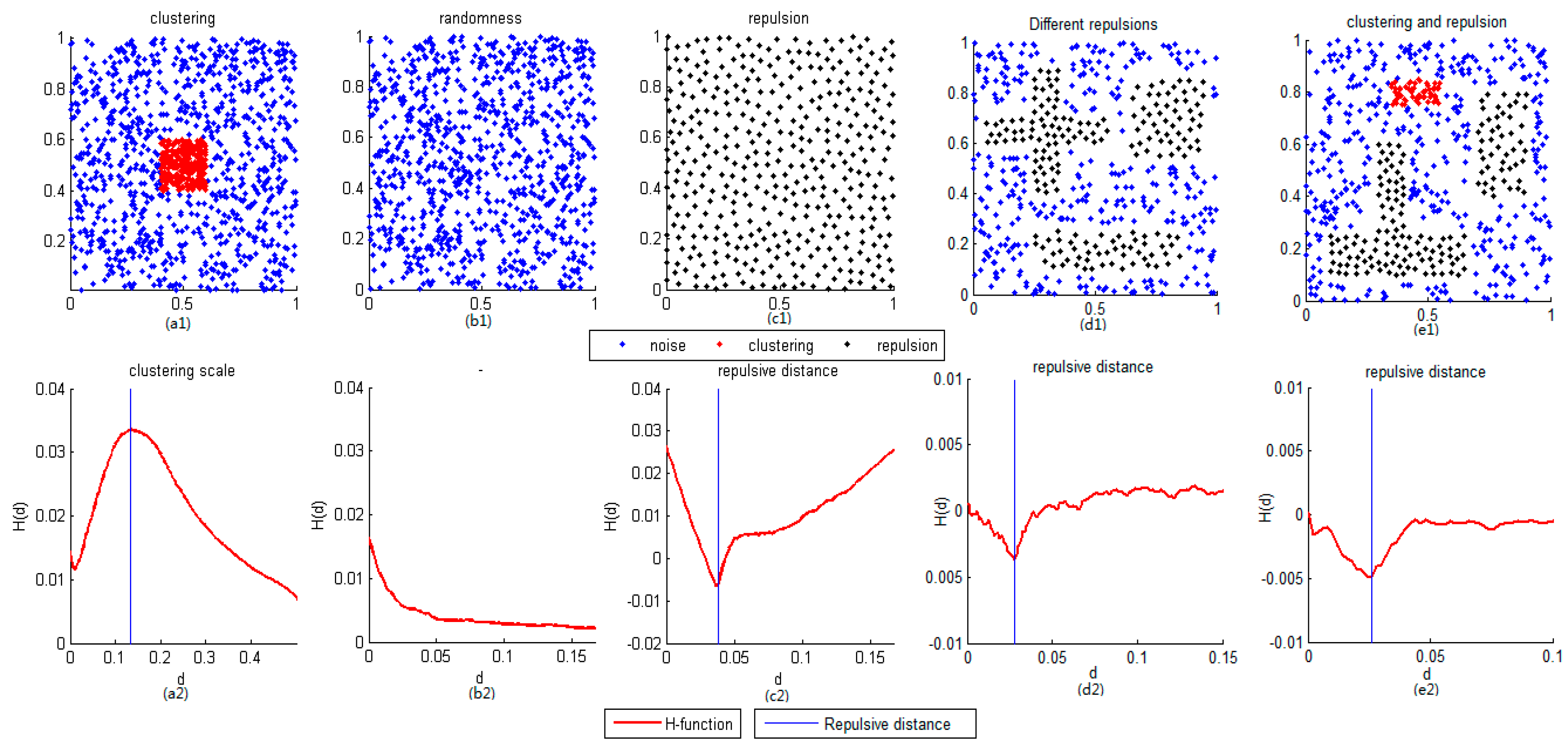
2.2.1. Determining the Existence of Repulsive Clusters
2.2.2. Extracting Repulsive Points Based on the Repulsive Distance
2.2.3. Generating Density-Connected Repulsive Clusters
3. Simulation Results
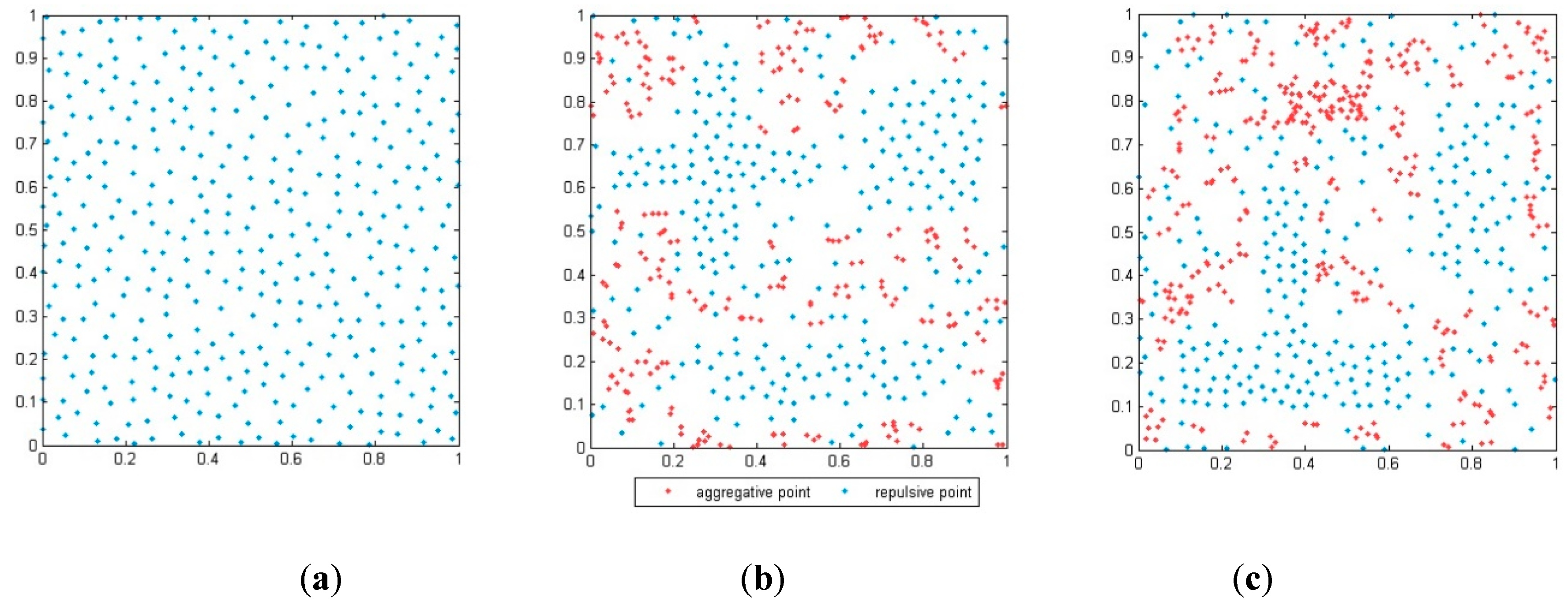
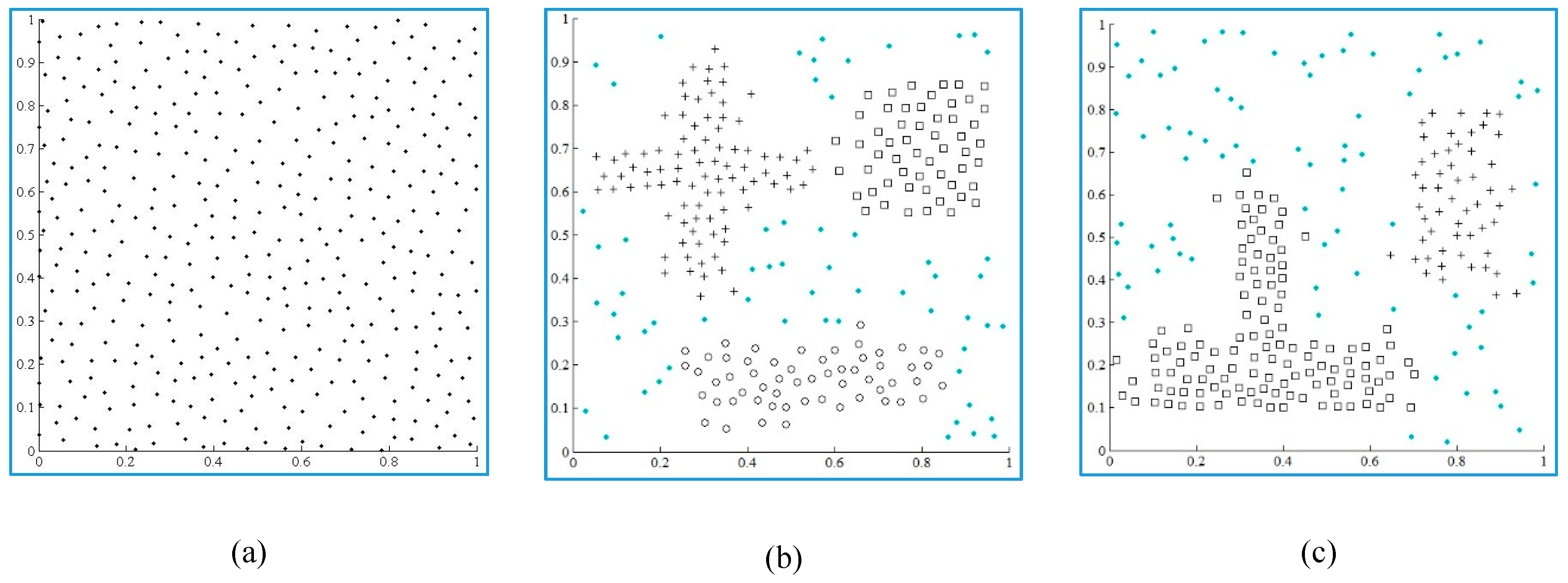
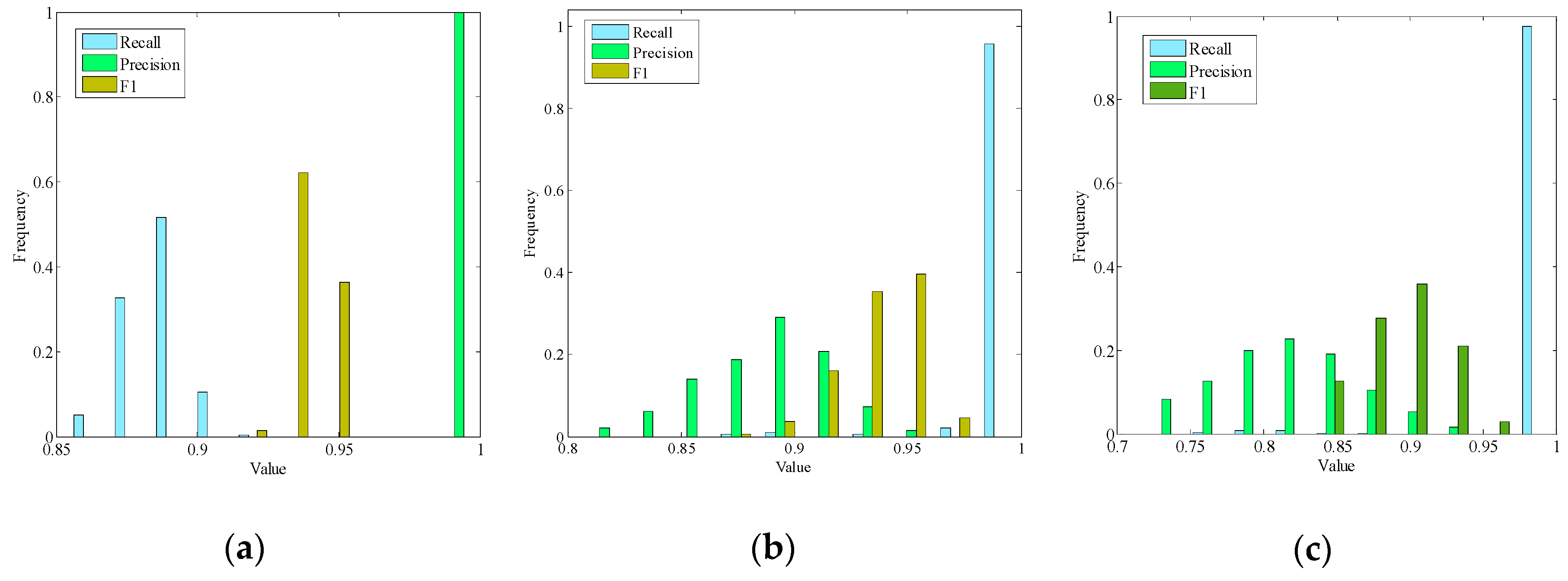
3.1. Validation of the Algorithm for Different Synthetic Datasets
3.2. Parameter Analysis
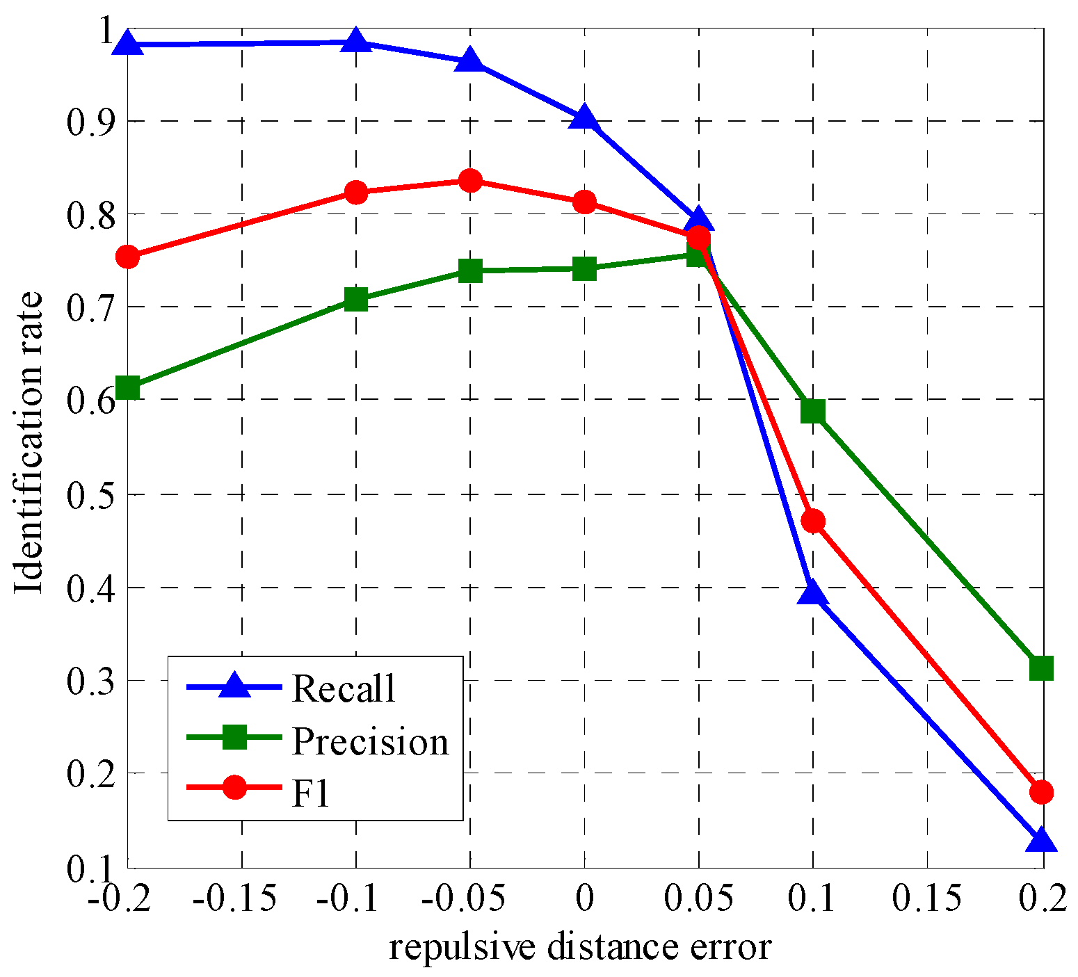
3.2.1. Effect of the Repulsive Distance on the Clustering Results
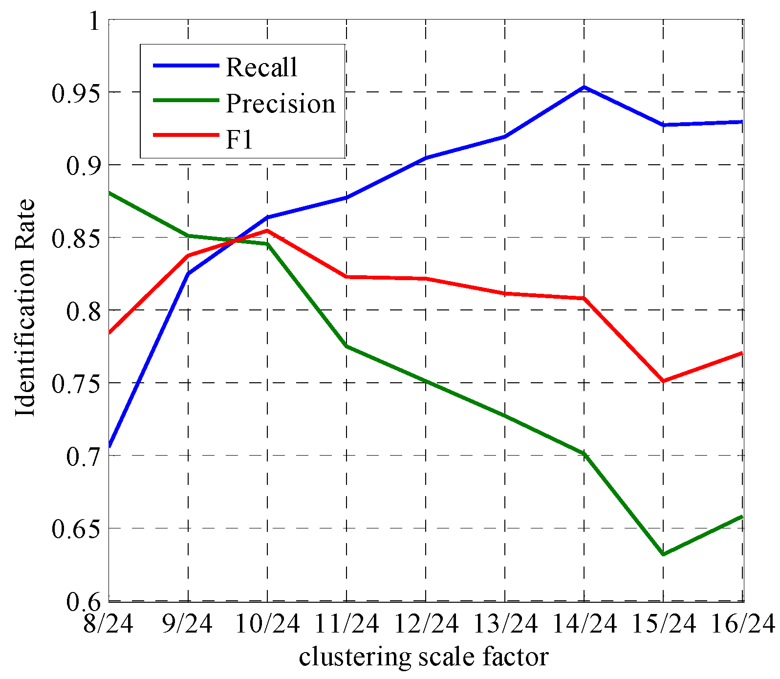
3.2.2. Effect of the Determination of Eps on the Clustering Results
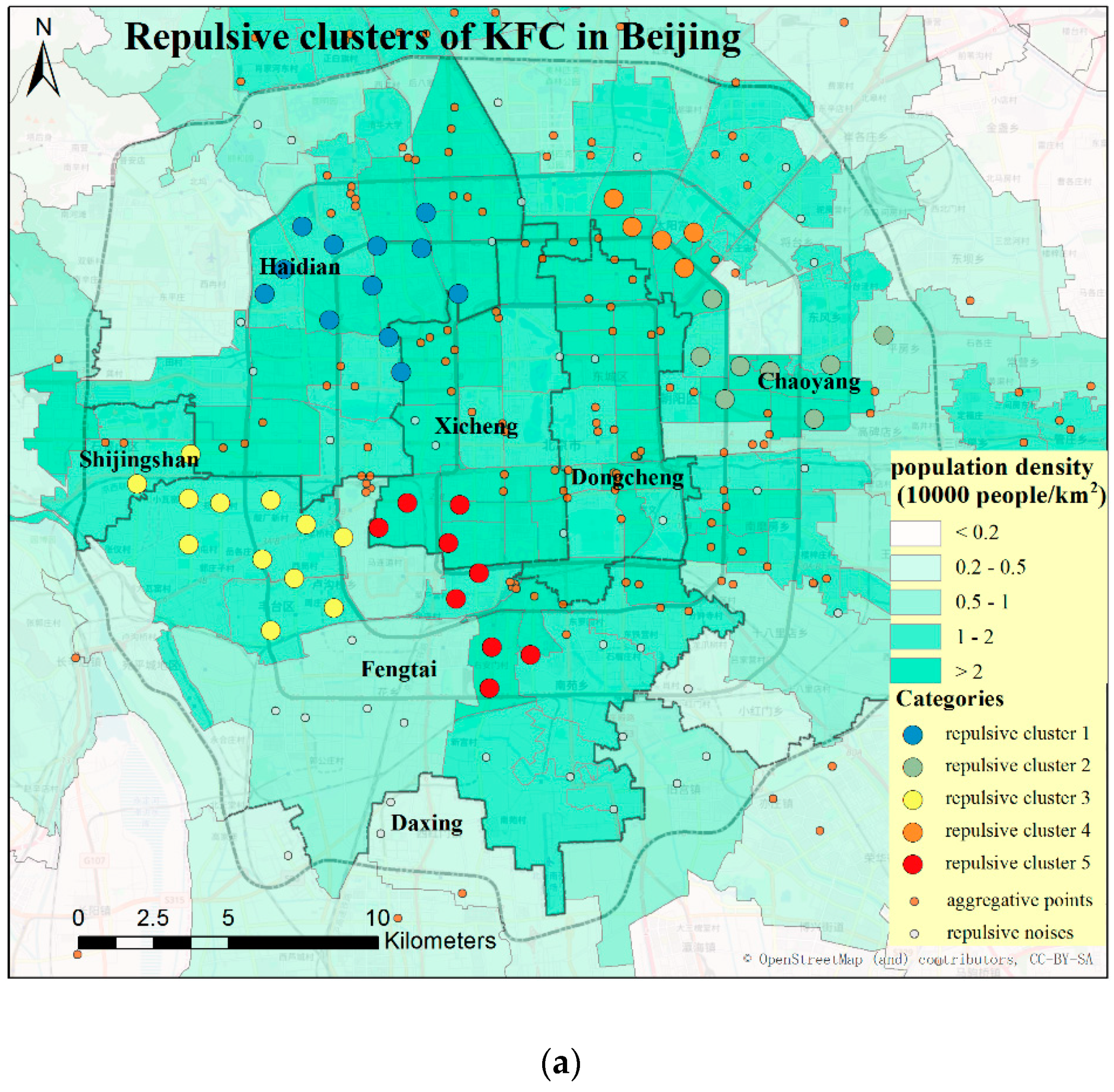
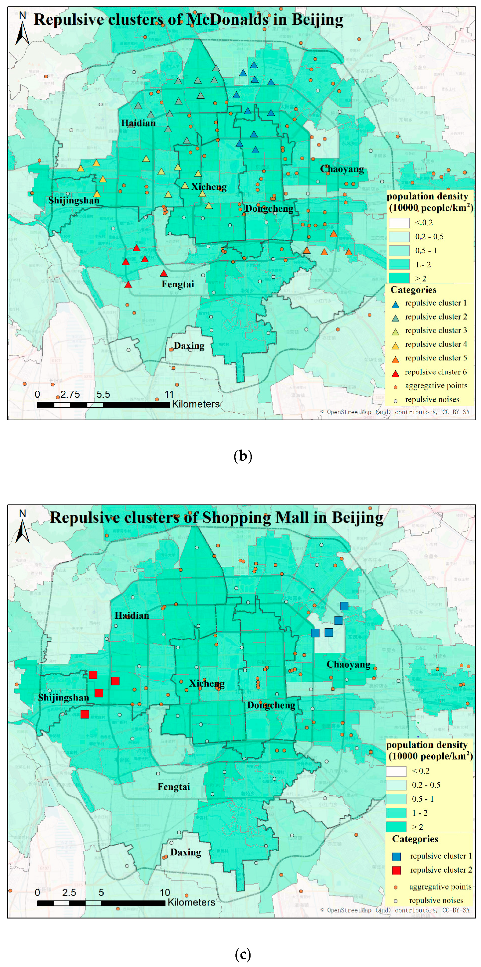
4. Case Study and Discussion
5. Conclusions
Author Contributions
Funding
Conflicts of Interest
References
- Pei, T.; Zhu, A.X.; Zhou, C.H.; Li, B.L.; Qin, C.Z. A new approach to the nearest-neighbour method to discover cluster features in overlaid spatial point processes. Int. J. Geogr. Inf. Sci. 2006, 20, 153–168. [Google Scholar] [CrossRef]
- Cheng, T.; Adepeju, M. Modifiable Temporal Unit Problem (MTUP) and its effect on space-time cluster detection. PLoS ONE 2014, 9, 1–10. [Google Scholar] [CrossRef] [PubMed]
- Adepeju, M.; Rosser, G.; Cheng, T. Novel evaluation metrics for sparse spatio-temporal point process hotspot predictions—A crime case study. Int. J. Geogr. Inf. Sci. 2016, 30, 2133–2154. [Google Scholar] [CrossRef]
- Han, J.W.; Kamber, M.; Tung, A.K.H. Spatial clustering methods in data mining. In Geographic Data Mining and Knowledge Discovery; Miller, H.J., Han, J.W., Eds.; Taylor & Francis: London, UK, 2001; pp. 188–217. [Google Scholar]
- Wiegand, T.; Moloney, K.A. Rings, circles, and null-models for point pattern analysis in ecology. Oikos 2004, 104, 209–229. [Google Scholar] [CrossRef]
- Lin, C.R.; Chen, M.S. Combining partitional and hierarchical algorithms for robust and efficient data clustering with cohesion self-merging. IEEE Trans. Knowl. Data Eng. 2005, 17, 145–159. [Google Scholar]
- Hinneburg, A.; Keim, D. An efficient approach to clustering in large multimedia databases with noise. In Proceedings of the 4th International Conference on Knowledge Discovery and Data Mining, New York, NY, USA, 27–31 August 1998; pp. 58–65. [Google Scholar]
- Karypis, G.; Han, E.H.; Kumar, V. Chameleon: Hierarchical clustering using dynamic modelling. IEEE Comput. 1999, 32, 68–75. [Google Scholar] [CrossRef]
- Ester, M.; Kriegel, H.P.; Sander, J.; Xu, X. A density-based algorithm for discovering clusters in large spatial databases with noise. In Proceedings of the 2nd International Conference on Knowledge Discovery and Data Mining, Portland, OR, USA, 2–4 August 1996; pp. 226–231. [Google Scholar]
- Ankerst, M.; Breunig, M.M.; Kriegel, H.P.; Sander, J. OPTICS: Ordering points to identify the clustering structure. Proceedings of ACM-SIGMOD ‘99 International Conference on Management Data, Philadelphia, PA, USA, 31 May–3 June 1999; pp. 46–60. [Google Scholar]
- Pei, T.; Gao, J.; Ma, T.; Zhou, C.H. Multi-scale decomposition of point process data. Geoinformatica 2012, 16, 625–652. [Google Scholar] [CrossRef]
- Sheikholeslami, G.; Chatterjee, S.; Zhang, A. WaveCluster: A multi-resolution clustering approach for very large spatial databases. In Proceedings of the 24th international conference on very large data bases, New York City, NY, USA, 24–27 August 1998; pp. 428–439. [Google Scholar]
- Estivill-Castro, V.; Lee, I. Multi-level clustering and its visualization for exploratory spatial analysis. GeoInformatica 2002, 6, 123–152. [Google Scholar] [CrossRef]
- Pei, T.; Zhou, C.H.; Zhu, A.X.; Li, B.L.; Qin, C.Z. Windowed nearest-neighbour method for mining spatiotemporal clusters in the presence of noise. Int. J. Geogr. Inform. Sci. 2010, 24, 925–948. [Google Scholar] [CrossRef]
- Pei, T.; Jasra, A.; Hand, D.J.; Zhu, A.X.; Zhou, C.H. DECODE: A new method for discovering clusters of different densities in spatial data. Data Min. Knowl. Discov. 2009, 18, 337–369. [Google Scholar] [CrossRef]
- Eberhardt, L.L. Some developments in ‘distance sampling’. Biometrics 1967, 23, 207–216. [Google Scholar] [CrossRef] [PubMed]
- Johnson, R.B.; Zimmer, W.J. A more powerful test for dispersion using distance measurements. Ecology 1985, 6, 1669–1675. [Google Scholar] [CrossRef]
- Pascual, D.; Pla, F.; Sanchez, J.S. Non parametric local density-based clustering for multimodal overlapping distributions. Proceedings of Intelligent Data Engineering and Automated Learning—IDEAL2006, Burgos, Spain, 20–23 September 2006; pp. 671–678. [Google Scholar]
- Prayag, V.R.; Deshmukh, S.R. Testing randomness of spatial pattern using Eberhardt’s index. Environmetrics 2000, 11, 571–582. [Google Scholar] [CrossRef]
- Schiffers, K.; Schurr, F.M.; Tielborger, K.; Urbach, C.; Moloney, K.; Jeltsch, F. Dealing with virtual aggregation—A new index for analysing heterogeneous point patterns. Ecography 2008, 31, 545–555. [Google Scholar] [CrossRef]
- Besag, J.E.; Gleaves, J.T. On the detection of spatial pattern in plant communities. Bull. Int. Stat. Inst. 1973, 45, 153–158. [Google Scholar]
- Ripley, B.D. Modelling spatial patterns. J. R. Stat. Soc. B 1977, 39, 172–192. [Google Scholar] [CrossRef]
- Ashour, W.; Sunoallah, S. Multi density DBSCAN. Lect. Notes Comput. Sci. 2011, 6936, 446–453. [Google Scholar]
- Jiang, H.; Li, J.; Yi, S.H.; Wang, X.Y.; Hu, X. A new hybrid method based on partitioning-based DBSCAN and ant clustering. Expert Syst. Appl. 2011, 38, 9373–9381. [Google Scholar] [CrossRef]
- Pielou, E.C. The use of plant-to-neighbour distances for the detection of competition. J. Ecol. 1962, 50, 357–367. [Google Scholar] [CrossRef]
- Getzin, S.; Dean, C.; He, F.; Trofymow, J.A.; Wiegand, K.; Wiegand, T. Spatial patterns and competition of tree species in a Douglas-fir chronosequence on Vancouver Island. Ecography 2006, 29, 671–682. [Google Scholar] [CrossRef]
- Wakefield, E.D.; Owen, E.; Baer, J.; Carroll, M.J.; Daunt, F.; Dodd, S.G.; Green, J.A.; Guilford, T.; Mavor, R.A.; Miller, P.I.; et al. Breeding density, fine-scale tracking, and large-scale modeling reveal the regional distribution of four seabird species. Ecol. Appl. 2017, 27, 2074–2091. [Google Scholar] [CrossRef] [PubMed]
- Flint, I.; Kong, H.; Privault, N.; Wang, P.; Niyato, D. Analysis of heterogeneous wireless networks using poisson hard-core hole process. IEEE Trans. Wirel. Commun. 2017, 16, 7152–7167. [Google Scholar] [CrossRef]
- Kwate, N.O.; Loh, J.M. Fast food and liquor store density, co-tenancy, and turnover: Vice store operations in Chicago, 1995–2008. Appl. Geogr. 2016, 67, 1–13. [Google Scholar] [CrossRef]
- Neyman, J. Statistical approach to problems of cosmology. J. R. Stat. Soc. 1958, 20, 1–43. [Google Scholar] [CrossRef]
- Spatenkova, O.; Stein, A. Identifying factors of influence in the spatial distribution of domestic fires. Int. J. Geogr. Inf. Sci. 2010, 24, 841–858. [Google Scholar] [CrossRef]
- Teichmann, J.; Ballani, F.; van den Boogaart, K.G. Generalizations of Matérn’s hard-core point processes. Spat. Stat. 2013, 3, 33–53. [Google Scholar] [CrossRef]
- Clark, P.J.; Evans, F.C. Distance to nearest neighbor as a measure of spatial relationships in populations. Ecology 1954, 35, 445–453. [Google Scholar] [CrossRef]
- Shu, H.; Pei, T.; Song, C.; Ma, T.; Du, Y.Y.; Fan, Z.D.; Guo, S.H. Quantifying the spatial heterogeneity of points. Int. J. Geogr. Inf. Sci. 2019, 33, 1355–1376. [Google Scholar] [CrossRef]
- Ripley, B.D. The second-order analysis of stationary point processes. J. Appl. Probab. 1976, 13, 255–266. [Google Scholar] [CrossRef]
- Besag, J.E. Comments on Ripley’s paper. J. R. Stat. Soc. B 1977, 39, 193–195. [Google Scholar]
- Kiskowski, M.A.; Hancock, J.F.; Kenworthy, A.K. On the use of Ripley’s K-function and its derivatives to analyze domain size. Biophys. J. 2009, 97, 1095–1103. [Google Scholar] [CrossRef] [PubMed]
- Pei, T.; Wang, W.Y.; Zhang, H.C.; Ma, T.; Du, Y.Y.; Zhou, C.H. Density-based clustering for data containing two types of points. Int. J. Geogr. Inf. Sci. 2015, 29, 175–193. [Google Scholar] [CrossRef]
- O’Haver, T. A Pragmatic Introduction to Signal Processing; CreateSpace Independent Publishing Platform: North Charleston, SC, USA, 1997. [Google Scholar]


| Dataset | Clusters | Number of Points | TP | FP | FN | Recall | Precision |
|---|---|---|---|---|---|---|---|
| Group I | All points | 400.5 | 354.76 | 0 | 45.71 | 88.6% | 100% |
| Group II | Square-Shaped Cluster | 53.94 | 53.67 | 13.35 | 0.28 | 99.5% | 88.2% |
| Strip-Shaped Cluster | 53.99 | 52.92 | 7.01 | 1.08 | 98.0% | 89.6% | |
| Cross-Shaped Cluster | 80.98 | 80.57 | 19.18 | 0.41 | 99.5% | 83.1% | |
| Noise Cluster | 0.00 | 0.00 | 2.93 | 0.00 | 0.0% | 0.0% | |
| All | 188.92 | 187.80 | 24.00 | 2.24 | 99.4% | 88.8% | |
| Group III | Bar-Square | 48.07 | 47.33 | 12.04 | 0.74 | 98.4% | 83.2% |
| Reversed “T”-Shaped Cluster | 105.37 | 100.73 | 20.00 | 4.64 | 95.4% | 84.0% | |
| Noise Cluster | 0.00 | 0.00 | 8.43 | 0.00 | 0.0% | 0.0% | |
| All | 153.63 | 148.96 | 35.55 | 9.33 | 96.9% | 81.2% |
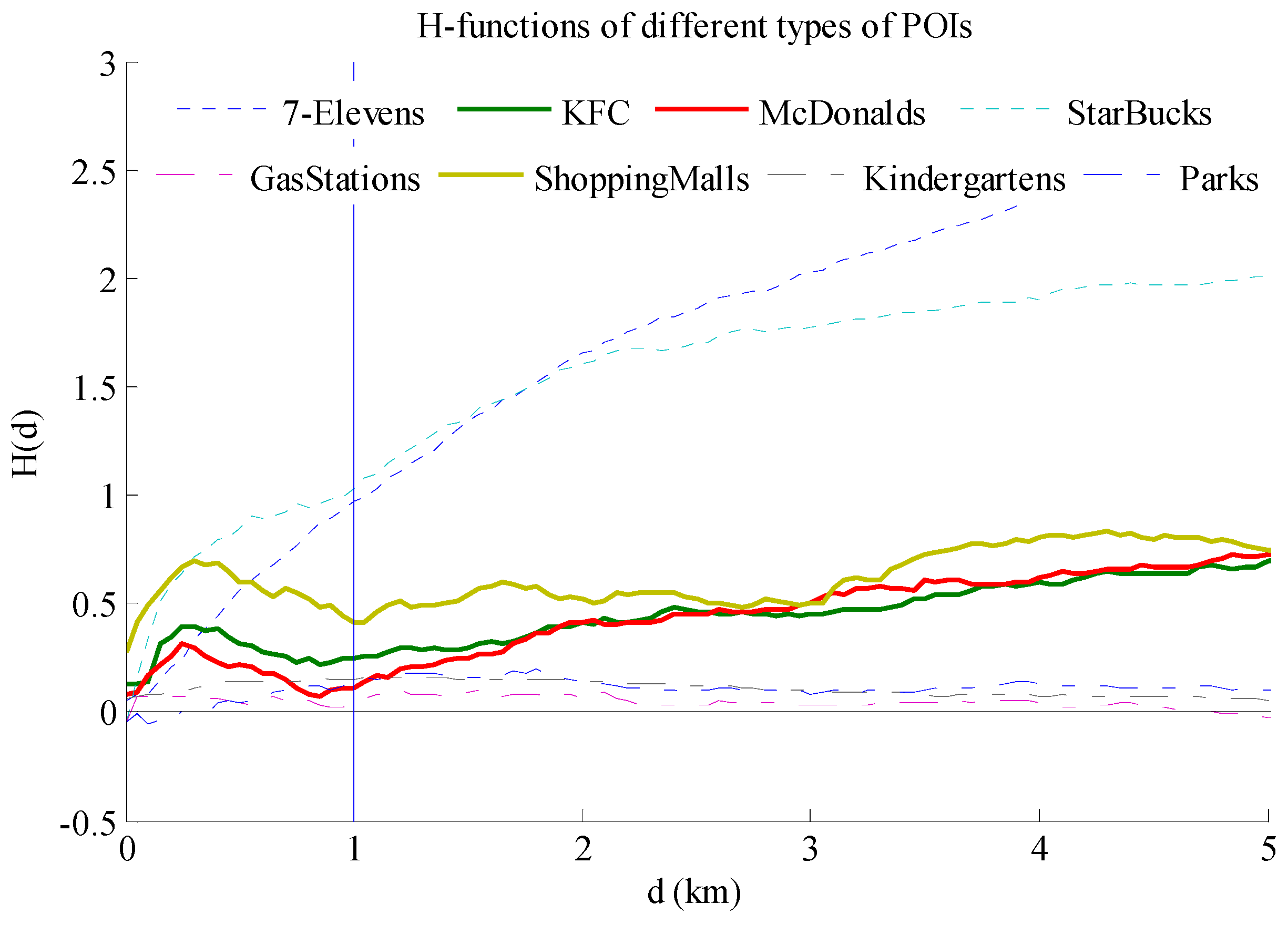
| POI Types | Number of Points | H-function | Clark and Evan’s A | Clustering Patterns |
|---|---|---|---|---|
| 7-Elevens | 195 | uptrend | 0.63 *** | Aggregative |
| KFC | 200 | d = 0.9 km | 0.94 * | Mixed |
| McDonalds | 156 | d = 1 km | 0.99 | Repulsive |
| Starbucks | 191 | uptrend | 0.62 *** | Aggregative |
| Gas Stations | 260 | - | 1.04 | - |
| Shopping Malls | 128 | d = 1.05 km | 0.80 *** | Mixed |
| Kindergartens | 830 | - | 0.88 *** | Aggregative |
| Parks | 216 | - | 0.99 | - |
© 2019 by the authors. Licensee MDPI, Basel, Switzerland. This article is an open access article distributed under the terms and conditions of the Creative Commons Attribution (CC BY) license (http://creativecommons.org/licenses/by/4.0/).
Share and Cite
Song, C.; Pei, T. Decomposition of Repulsive Clusters in Complex Point Processes with Heterogeneous Components. ISPRS Int. J. Geo-Inf. 2019, 8, 326. https://doi.org/10.3390/ijgi8080326
Song C, Pei T. Decomposition of Repulsive Clusters in Complex Point Processes with Heterogeneous Components. ISPRS International Journal of Geo-Information. 2019; 8(8):326. https://doi.org/10.3390/ijgi8080326
Chicago/Turabian StyleSong, Ci, and Tao Pei. 2019. "Decomposition of Repulsive Clusters in Complex Point Processes with Heterogeneous Components" ISPRS International Journal of Geo-Information 8, no. 8: 326. https://doi.org/10.3390/ijgi8080326
APA StyleSong, C., & Pei, T. (2019). Decomposition of Repulsive Clusters in Complex Point Processes with Heterogeneous Components. ISPRS International Journal of Geo-Information, 8(8), 326. https://doi.org/10.3390/ijgi8080326