Spatial Disaggregation of Historical Census Data Leveraging Multiple Sources of Ancillary Information

Abstract

High-resolution population grids built from historical census data can ease the analyses of geographical population changes, at the same time also facilitating the combination of population data with other GIS layers to perform analyses on a wide range of topics. This article reports on experiments with a hybrid spatial disaggregation technique that combines the ideas of dasymetric mapping and pycnophylactic interpolation, using modern machine learning methods to combine different types of ancillary variables, in order to disaggregate historical census data into a 200 m resolution grid. We specifically report on experiments related to the disaggregation of historical population counts from three different national censuses which took place around 1900, respectively in Great Britain, Belgium, and the Netherlands. The obtained results indicate that the proposed method is indeed highly accurate, outperforming simpler disaggregation schemes based on mass-preserving areal weighting or pycnophylactic interpolation. The best results were obtained using modern regression methods (i.e., gradient tree boosting or convolutional neural networks, depending on the case study), which previously have only seldom been used for spatial disaggregation.

1. Introduction

Accurate information about the human population distribution is essential for formulating informed hypothesis in the context of population-related social, economic, and environmental issues. For geographers, historians, and social scientists, it is important to have access to population information at specific temporal snapshots, and often also across long periods of time. An authoritative source of population data are government instigated national censuses, which subdivide the geographical space into discrete areas (e.g., fixed national administrative units) and provide multiple snapshots of society at regular intervals, typically every 10 years. Many research institutions or national statistical offices have developed historical geographical information systems, which contain statistical data from previous censuses together with the administrative boundaries (i.e., records of administrative boundary changes over time) used to publish them over long periods of time. However, using these data when looking at changes over time remains quite challenging, for the most part due to difficulties in handling the boundaries of the administrative units that were used for publishing the data.

There are several applications where population data aggregated to fixed administrative units is not an ideal form of information about population counts and/or density. First, these representations are more sensitive to modifiable areal unit problems, in the sense that the results of an analysis based on data aggregated by administrative units may depend on the scale, shape, and arrangement of the units, rather than capturing the theoretically continuous variation in the underlying population [1,2]. Although raster-based representations are also affected by these problems, they offer regularly sized units, and considering a high resolution we can better handle scale issues [2]. Secondly, the spatial detail of aggregated data is variable and usually low, particularly in the context of historical data. In a highly-aggregated form these data are useful for broad-scale assessments, but using aggregated data can mask important local hotspots, and overall tends to smooth out spatial variations. Third, there is often a spatial mismatch between census areal units and the user-desired units that are required for particular types of analysis. Finally, the boundaries of census aggregation units may change over time from one census to another, making the analysis of population change, in the context of longitudinal studies dealing with high spatial resolutions somewhat difficult.

Given the aforementioned limitations, high-resolution population grids (i.e., geographically referenced lattices of square cells, with each cell carrying a population count or the value of population density at its location) are often used as an alternative format to deliver population data [3]. All cells in a population grid have the same size and the cells are stable in time. There are no spatial mismatches as study areas can be rasterized to be co-registered with a population grid.

Population grids can be built from national census data through spatial disaggregation methods, which range in complexity from simple mass-preserving areal weighting [4], to intelligent dasymetric weighting schemes that leverage regression analysis to combine multiple sources of ancillary data [3,5]. Nowadays, there are for instance many well-known gridded datasets that describe modern population distribution, created using a variety of disaggregation techniques. These include the Gridded Population of the World [6], LandScan [7], Global Human Settlement [8,9,10,11], GRUMP [12], SocScape [13], and the WorldPop [14,15,16,17] databases. However, despite the rapid progress in terms of spatial disaggregation techniques, population grids have not been widely adopted in the context of historical data. Studies looking at population changes over long temporal periods manipulate the data for the sake of spatio-temporal consistency, but the typical procedures involve harmonizing the data to standard boundaries (e.g., using areal interpolation methods to transform the historical data into modern administrative units, allowing contemporary population patterns to be understood in the light of the historical changes [18,19]), instead of relying on disaggregation methods for producing raster representations. We argue that the availability of high-resolution population grids within historical geographical information systems (GIS) has the potential to improve the analyses of long-term geographical population changes and, more importantly, to facilitate the combination of population data with other GIS layers to perform analyses on a wide range of topics, such as the development of the transport network [19,20,21], or the formation of urban agglomerations.

In this article, we report on experiments with a hybrid spatial disaggregation technique that combines the ideas of dasymetric mapping and pycnophylactic interpolation, using machine learning methods (e.g., ensembles of decision trees [22] or deep learning methods based on convolutional neural networks [23,24]) to combine different types of ancillary data, in order to disaggregate historical census data into a 200 m resolution grid. Apart from few exceptions related to the use of areal interpolation for integrating historical census data [18,25,26,27,28,29], most previous studies concerning with spatial disaggregation have focused on modern datasets.

We specifically report on experiments related to the disaggregation of historical population counts from three different national censuses which took place around 1900, respectively in Great Britain, Belgium, and the Netherlands. All three statistical datasets, together with the corresponding boundaries for the regions at which the data were collected (i.e., parishes or municipalities), are presently available in digital formats within national historical GIS projects. This historical period (i.e., the changeover from the 19th to the 20th century, often referred to as the Belle Epoque) is also particularly interesting, being for instance characterized by strong urbanization and a rising factory proletariat (e.g., we can expect different terrain characteristics to be able to inform estimates of population distribution).

The rest of this document is organized as follows: Section 2 briefly overviews related work in the area. Section 3 presents the general spatial disaggregation method that was used in our study, together with the sources of ancillary information that have been explored. Section 4 presents experimental results obtained from the application of the proposed method to the aforementioned three different historical datasets, related to the territories of Great Britain, Belgium, and the Netherlands. Finally, Section 5 summarizes our conclusions and presents possible directions for future work.

2. Fundamental Concepts and Related Work

Spatial disaggregation and the creation of high-resolution grids with the human population distribution have been studied for decades [3]. Nowadays, there are, for instance, many well-known gridded datasets that describe the modern human population distribution, created using a variety of spatial disaggregation techniques [6,7,14,15,16,17].

The simplest spatial disaggregation method is perhaps mass-preserving areal weighting, whereby the known population of source administrative regions is divided uniformly across their area, in order to estimate population at target regions of higher spatial resolution [4]. The process usually relies on a discretized grid over the administrative regions, where each cell in the grid is assigned a value equal to the total population over the number of cells that cover the corresponding administrative region. Pycnophylactic interpolation is a refinement of mass-preserving areal weighting that assumes a degree of spatial auto-correlation in the population distribution [30]. This method starts by applying the mass-preserving areal weighting procedure, afterward smoothing the values for the resulting grid cells by replacing them with the average of their neighbors. The aggregation of the predicted values for all cells within a source region is then compared with the actual value, and adjusted to keep the consistency within the source regions. The method continues iteratively until there is either no significant difference between predicted values and actual values within the source regions, or until there have been no significant changes from the previous iteration.

Dasymetric weighting schemes are instead based on creating a weighted surface to distribute the known population, instead of considering a uniform distribution as in mass-preserving areal weighting. Dasymetric weighting schemes are usually determined by combining different spatial layers (e.g., terrain elevation and/or slope, land versus water masks, etc.) according to rules that relate the ancillary variables to expected population counts. While some weighting schemes use simple binary masks built from land-coverage data, other approaches rely on expert knowledge and manually-defined rules, and more recent methods leverage machine learning to improve upon the heuristic definition of weights/rules [5,17,31,32], often combining many different sources of ancillary information (e.g., satellite imagery of night-time lights [17,33], LIDAR-derived building volumes [34,35], or even density maps derived from geo-referenced tweets [4], from OpenStreetMap points-of-interest [36], or from mobile phone usage data [37]).

Although several previous dasymetric mapping methods have explored machine learning approaches for defining the weights, only a few of these previous studies have explored the use of deep learning approaches. The study from Tiecke et al. [38] is one of these exceptions, describing a spatial desegregation method for producing population maps (i.e., the authors described the production of maps depicting population counts for 18 countries at a resolution of approximately 30 m) that first leverages a convolutional neural network for detecting/delimiting individual buildings in high-resolution satellite imagery, and then uses the building estimates as a mask for proportionally allocating population counts (i.e., census counts are distributed proportionally through a dasymetric approach, using the fraction of built-up area within each 30 m grid cell). Image patches of $64\times 64$ pixels are first extracted from satellite imagery around straight lines, using a conventional edge detector. Limiting the analysis to these patches significantly reduces the amount of data for classification. A portion of the patches was sampled and labeled by human-experts, in order to support the training of the methods for detecting building footprints. A combination of two CNN models, based on the previously proposed SegNet [39] and FeedbackNet [40] architectures, is used at this stage, and the results are finally used for population redistribution.

The previous studies concerned with spatial disaggregation that are perhaps most similar to the present work are those from Monteiro et al. [5], in which a general machine learning method that combines pycnophylactic interpolation and dasymetric weighting is presented, and from Robinson et al. [41] and Doupe et al. [42], which also use deep learning models for estimating population from satellite imagery. The present article extends on the work reported by Monteiro et al., applying a hybrid disaggregation procedure to historical data, and evaluating the effectiveness of different machine learning methods, including state-of-the-art approaches based on ensembles of decision trees or deep convolutional neural networks. Given that we address the generation of high-resolution raster representations covering large geographical extents, the present study also explores high-performance computing methods, so that results can be produced in a useful amount of time. Our efforts in terms of computational efficiency include the parallel implementation of pycnophylactic interpolation, which is used for the initialization of our full approach, and the parallel inference and application of machine learning models. Besides parallelization, we also considered the use of secondary memory, in order to process raster datasets that do not fit entirely in memory.

Spatial disaggregation and areal interpolation methods have also been previously explored in the context of historical data, for instance to estimate population in one census year (i.e., the source regions) within the units of another year (i.e., the target regions), in order to construct temporally consistent small census units [18,19,25,26,27,28,29]. However, most previous studies have only considered simple approaches that do not rely on machine learning for inferring dasymetric weights (e.g., most modern approaches involve the use of satellite imagery not available in historical contexts, although other sources of information can perhaps be used instead). For instance, in the context of the Great Britain Historical Geographical Information Systems (GBHGIS), Gregory described an areal interpolation method based on the expectation-maximization (EM) algorithm, aiming to standardize 19th and 20th century census data by converting the regions from all dates onto a single set of regions corresponding to registration districts in the U.K., to allow long-term comparisons [25]. The proposed approach involves first dividing the study area into control regions (i.e., parishes), initially having the same population density. In the expectation step of the EM algorithm, the population of each zone of intersection between the source regions and the control regions is estimated according to mass-preserving areal weighting. Then, the Maximization step uses maximum likelihood to estimate the population densities of each control region, based on the results of the E step. The resulting information is then fed back to the E step, where the populations of the zones of intersection are re-estimated. The algorithm is repeated until convergence.

In summary, the present study extends previous efforts related to spatial disaggregation, focusing on the application to historical datasets. We describe methods for the creation of high-resolution population grids (i.e., 200 m per cell, representing a balance between the resolutions associated to the different ancillary datasets that were considered to support the disaggregation procedure, and that although being much coarser lower than the resolution used in the study by Tiecke et al. [38] leveraging deep neural networks and high-resolution satellite imagery, is still slightly higher than the 250 m resolution used in the modern WorldPop dataset), using dasymetric weighting approaches based on state-of-the-art machine learning methods, and evaluating the impact of using different sources of ancillary information, including historical land coverage data [43,44] and modern information that may correlate with the historical population.

3. The Proposed Hybrid Disaggregation Method

In this article, envisioning the disaggregation of historical census data, we propose to leverage a hybrid approach that combines pycnophylactic interpolation and regression-based dasymetric mapping, following the general ideas that were advanced by Monteiro et al. [5]. In brief, pycnophylactic interpolation is used for producing initial estimates from the aggregated data, which are then adjusted through an iterative procedure that uses regression modeling to infer population from a set of ancillary variables. The general procedure is illustrated in Figure 1 and detailed next, through an enumeration of all the individual steps that are involved:

• Produce a vector polygon layer for the data to be disaggregated by associating the population counts, linked to the source regions, to geometric polygons representing the regions;
• Create a raster representation for the study area, with basis on the vector polygon layer from the previous step and considering a resolution of 200 m per cell. This raster, referred to as $T^p$, will contain smooth values resulting from a pycnophylactic interpolation procedure [30]. The algorithm starts by assigning cells to values computed from the original vector polygon layer, using a simple mass-preserving areal weighting procedure (i.e., we re-distribute the aggregated data with basis on the proportion of each source zone that overlaps with the target zone). Iteratively, each cell’s value is replaced with the average of its 8 neighbors in the target raster. We finally adjust the values of all cells within each zone proportionally, so that each zone’s total in the target raster is the same as the original total (e.g., if the total is 10% lower than the original value, we increase the value of each cell by a factor of 10%). The procedure is repeated until no significant changes occur. The resulting raster is a smooth surface corresponding to an initial estimate for the disaggregated values;
• Overlay six rasters of ancillary data, $P^1$, $P^2$, $P^3$, $P^4$, $P^5$ and $P^6$, also using a resolution of 200 m per cell, on the study region from the original vector layer and from the raster produced in the previous step. These rasters contain information regarding (i) modern population density, (ii) historical land coverage, (iii) terrain elevation, (iv) modern data on terrain development, (v) modern data on human settlements, and (vi) distance from a given cell to the nearest cell with a land coverage equal to water. These data were used as ancillary information for the spatial disaggregation procedure. Prior to overlaying the data, the six different raster sources are normalized to the resolution of 200 m per cell, through an aggregation procedure based on averaging the different encompassed cells (i.e., in the cases where the original raster had a higher resolution), or through the application of bi-linear [45] interpolation (i.e., in the cases where the original raster had a lower resolution, and producing smoother results than those obtained by taking the value from the nearest/encompassing cell);
• Overlay another raster $T^d$ on the study region, with the same resolution used in the rasters from the previous steps (i.e., 200 m per cell). This raster will be used to store the estimates produced by a simple spatial disaggregation procedure leveraging rule-based dasymetric mapping (i.e., a method based on proportional and weighted areal interpolation). For producing these estimates, we weight the total value, for each source zone in the original vector polygon layer, according to the proportion between the modern population counts available for the corresponding cell in raster $P^1$, and the sum of all the values for the given source zone in the same raster. This is essentially a proportional and weighted areal interpolation method, corresponding to Equation (1) and where $T_t^d$ is the estimated count in target zone t, where $S_s$ is the historical population count in source zone s, $P_t$ is the modern population count in target zone t, and $P_s$ is the modern population count in source zone s;

  $$T_t^d=\sum _{\{s:s\cap t\ne \varnothing \}}\left(\frac{P_t}{P_s}\times S_s\right).$$

  (1)
• Create a final raster overlay, through the application of an intelligent dasymetric disaggregation procedure based on disseveration, originally proposed by Malone et al. [46] and later extended by Roudier et al. [47] and by Monteiro et al. [5]. The algorithm leverages the rasters from the previous steps as ancillary information. Specifically, the vector polygon layer from step 1 is considered as the source data to be disaggregated, while raster $T^p$ from step 2 is considered as an initial estimate for the disaggregated values. Rasters $P^1$ to $P^6$, as well as raster $T^d$, are seen as predictive covariates. The regression algorithm used in the disseveration procedure is fit using the available data, and applied to produce new values for raster $T_p$. The application of the regression algorithm will refine the initial estimates with basis on their relation towards the predictive covariates, this way dissevering the source data into the target raster cells;
• Proportionally adjust the values returned by the down-scaling method from the previous step for all cells within each source zone, so that each source zone’s total in the target raster is the same as the total in the original vector polygon layer (e.g., again, if the total is 10% lower than the original value, increase the value of each cell in by a factor of 10%).
• Steps 5 to 7 are repeated, iteratively executing the disseveration procedure that relies on regression analysis to adjust the initial estimates $T^p$ from step 2, until the estimated values converge (i.e., until the change in the estimated error rate over three consecutive iterations is less than 0.001) or until reaching a maximum number of iterations (i.e., 200 iterations).

Notice that the previous enumeration describes the proposed procedure through example applications that involve a specific resolution (i.e., 200 m per cell) and a particular set of ancillary datasets. The same general procedure could nonetheless also be used in different scenarios, involving different parameters. Moreover, different regression algorithms can also be used in step 6. The following sub-sections describe the particular regression algorithms that were considered, and detail the different sources of ancillary data.

3.1. Implementation Details and the Considered Regression Algorithms

The aforementioned procedure was implemented through the programming language of the R (http://www.r-project.org) project for statistical computing. Given that there are already many extension packages (http://cran.r-project.org/web/views/Spatial.html) for R concerned with the analysis of spatial data, using R facilitated the use of geo-spatial datasets encoded using either the geometric or the raster data models. We have specifically integrated and extended the source code from the R packages named pycno (http://cran.r-project.org/web/packages/pycno/) and dissever (http://github.com/pierreroudier/dissever), which respectively implement the pycnophylactic interpolation algorithm from Tobler [30] used in step 2, and the down-scaling procedure based on regression analysis and disseveration, that was outlined by Malone et al. [46] and that was used in step 6. Specifically on what regards pycnophylactic interpolation, the implementation from the pycno package was extended in order to consider parallel processing, by dividing the target region into multiple slices that are processed independently in parallel (i.e., each worker thread is assigned to a slice of the entire geographic region, and the different slices overlap in one column in order to support accessing the neighboring cells that are processed by an independent worker thread).

The latest version of dissever is internally using the caret (http://cran.r-project.org/web/packages/caret) package, in terms of the implementation of the regression models. The caret package, short for classification and regression training, contains numerous tools for developing different types of predictive models, facilitating the realization of experiments with different types of regression approaches in order to discover the relations between the target variable and the available covariates. Leveraging caret, we specifically experimented with standard linear regression models, and with approaches based on ensembles of decision trees. We also extended the dissever package in order to use keras (http://rstudio.github.io/keras/) as an alternative machine learning library, which allowed us to experiment with the use of deep convolutional neural networks.

In standard linear regression, a linear least-squares fit is computed for a set of predictor variables (i.e., the covariates) to predict a dependent variable (i.e., the disaggregated values). The regression equation corresponds to a linear combination of the predictive covariates, added to a bias term.

In turn, models based on decision trees correspond to non-linear procedures based on inferring a flow-chart-like structure, where each internal node denotes a test on an attribute, each branch represents the outcome of a test, and each leaf node holds a target value. Decision trees can be learned by splitting the source set of training instances into subsets, based on finding an attribute value test that optimizes the homogeneity of the target variable within the resulting subsets (e.g., by optimizing an information gain metric). This process is recursively applied to each derived subset. Recently, ensemble strategies for combining multiple decision trees, extending the general concepts of boosting [48] or bagging [49], have become popular in machine learning and data mining competitions, often achieving state-of-the-art results while at the same time supporting efficient training and inference through the parallel training of the trees involved in the ensemble [22].

Specifically, the cubist approach combines decision trees with linear regression models, in the sense that the leaf nodes in these trees contain linear regression models based on the predictors used in previous splits [50]. There are also intermediate linear models at each step of a tree, so that the predictions made by the linear regression model, at the terminal node, are also smoothed by taking into account the predictions from the linear models in the previous nodes, recursively up the tree. The cubist approach is also normally used within an ensemble classification scheme based on boosting, in which a series of trees is trained sequentially with adjusted weights. The final predictions result from the average of the predictions from all committee members.

The gradient tree boosting approach also operates in a stage-wise fashion, in this case sequentially learning decision tree models that focus on improving the decisions of predecessor models. The prediction scores of each individual tree are summed up to get the final score. Chen and Guestrin introduced a scalable tree boosting library called XGBoost, which has been used widely by data scientists to achieve state-of-the-art results on many machine learning challenges [48]. XGBoost is available from within the caret package, and we used this specific implementation of tree boosting.

All three aforementioned procedures (i.e., linear regression modeling, cubist, and gradient tree boosting) process each grid cell independently of the others. The values for each cell of the raster grid $T^p$ are used to fit the parameters of a regression model, taking the values from the corresponding cells in the ancillary rasters as the predictor variables. 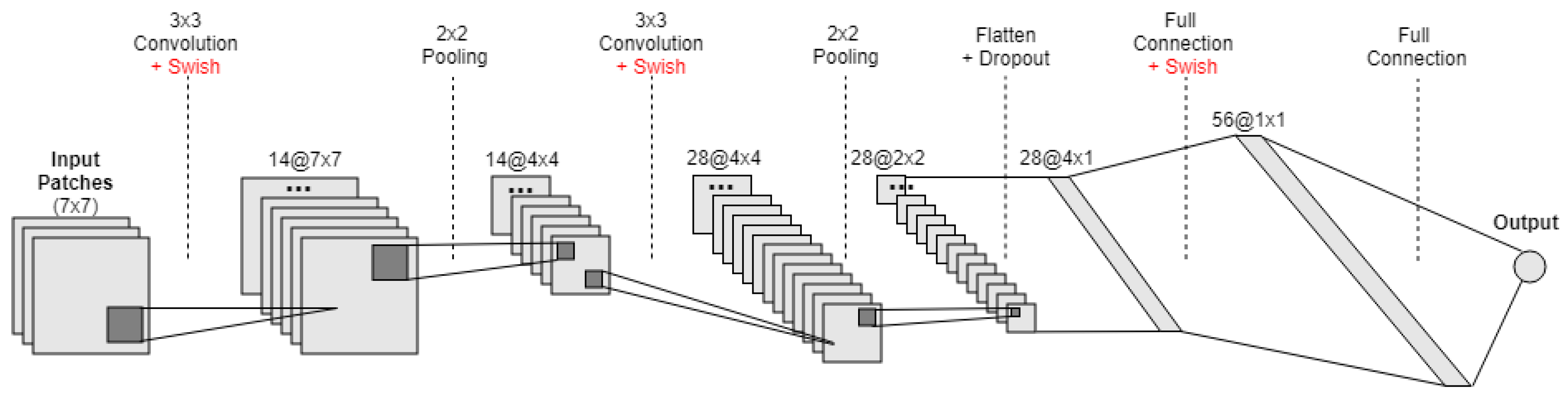The model is then used to update the value of each cell in the raster grid $T^p$, again leveraging the values from the corresponding cells in the ancillary rasters. Extending on this idea, we also experimented with a more sophisticated non-linear regression model, based on a deep convolutional neural network (CNN). The network takes input patches of $7\times 7$ grid cells (i.e., 49 cells in total, with each cell in the patch described by 7 values taken from the corresponding cells in the grids with the ancillary data—rasters $P^1$ to $P^6$, as well as raster $T^d$), in order to produce an estimate for the central cell in the patch. The considered CNN is based on the LeNet-5 architecture [24], which we describe next and is illustrated on Figure 2. The reader can refer to recent tutorials and surveys [23,51,52] for further information about deep learning with CNNs:

• The first hidden layer performed a two-dimensional convolution. The layer had 14 feature maps, each with the size of $3\times 3$, and it also used a recently proposed activation function named Swish [53]. This is the input layer, expecting patches with the structure outlined above;
• Next we defined a pooling layer that took the maximum values, configured with a pool size of $2\times 2$ and with a stride of 2. This was equivalent to a $2\times 2$ sliding window that walks across the activation volume, taking the maximum value of each region, while taking a step of two cells in both the horizontal and vertical directions;
• Afterwards, we had a second two-dimensional convolution layer, again with a filter size of $3\times 3$ and using the Swish activation function, but this time with 28 feature maps instead of 14;
• Then, we had another pooling layer similar to the previous one, again taking maximum values and with a pool size of $2\times 2$;
• Afterwards, we had a dropout regularization layer, configured to randomly exclude 10% of the neurons in order to reduce over-fitting;
• Next, we converted the 2D matrix resulting from the previous step to a flattened vector, allowing the data to be processed by standard fully-connected layers. We specifically used a fully-connected layer with 56 neurons and with the swish activation function;
• Finally, the output layer had one single neuron with a linear activation function, in order to output a real value corresponding to the estimated population at the center cell of the input patch.

Independently of the regression model being used, for performance reasons and also in accordance with the original implementation of the disseveration procedure [46,47], each iteration of the disaggregation method used a random sample with 25% of the cells (or 25% of the $7\times 7$ patches, in the case of the CNN model) as the training data for fitting the regression model. Different random samples are considered at each iteration of the disseveration procedure.

Some of the hyper-parameters involved on the different models (e.g., the number of trees in the ensemble methods that were used, or the learning rate in the CNN model) were also tuned for optimal performance at each iteration of the disseveration procedure. For instance, in the case of gradient tree boosting, the caret package was used to tune parameters such as the number of trees, the learning rate, or the minimum loss reduction required to make a further partition on a leaf node of a tree.

Specifically on what regards the CNN model, the training procedure used a loss function corresponding to the mean squared error, considering batches of 1024 instances, and using one epoch over the training data per iteration of the disseveration procedure. We used the Adam optimization algorithm [54] with the default parameters in the keras deep learning library, except for the learning rate which was set to ${10}^{-i}$, with i equal to 3, 4 or 5.

In order to avoid overfitting with the CNN model, besides using dropout regularization, we also used a data augmentation procedure for artificially creating new training instances, at each iteration of the dissever procedure. Assuming that different types of transformations on the input data (i.e., the patches containing ancillary data) can result on different representations for the same population count, we followed an approach that extends the original dataset in 2.5 times its original size. The new patches were computed by randomly applying, to each original training patch, (i) a vertical flip, (ii) an horizontal flip, (iii) both vertical and horizontal flips, (iv) a rotation of 90°, (v) a rotation of −90°, or (vi) a transpose operation.

3.2. The Ancillary Data Sources

Our disaggregation procedure leverages six different sources of external ancillary data (i.e., rasters $P^1$ to $P^6$ from the previous enumeration), specifically encoding (i) modern population density, (ii) historical land coverage, (iii) terrain elevation, (iv) modern data on terrain development, (v) modern data on human settlements, and (vi) distance from a given cell to the nearest cell with a land coverage type equal to water. All these six sources of information are expected to correlate with historical population density, although to different degrees. Figure 3 provides an illustration for the data available in all six sources, for a region corresponding to the territory of Great Britain.

The ancillary information regarding modern terrain development and modern population counts was obtained from the Global Human Settlement (GHS (http://ghsl.jrc.ec.europa.eu)) project [8,9,10,11], which focuses on mapping the distribution and density of the world’s built-up areas. This project analyzed Landsat imagery, related to the epochs of 1975, 1990, 2000 and 2013–2014, to quantify built-up structures in terms of their location and density. Raster grids with a resolution of 38 m per cell are made available through the project, expressing the distribution of built-up areas as the proportion (i.e., ratio) of occupied footprint in each cell. We specifically used the GHS built-up presence grid related to the year of 1975 (i.e., the oldest year for which data is available), converting the data to the resolution of 200 m per cell.

Besides the raster encoding terrain development (i.e., built-up presence), the GHS project also created population density grids for the same years, with a resolution of 250 m per cell. The methodology for building these grids was based on raster-based dasymetric mapping, using the GHS built-up presence to restrict and refine the population information available through the Gridded Population of the World (GPW (http://beta.sedac.ciesin.columbia.edu/data/collection/gpw-v4)) dataset. This population grid was in turn constructed from national or subnational input units (i.e., from low-level administrative units from the different countries) of varying resolutions, through a spatial disaggregation procedure. Since historical population counts are expected to correlate with modern population density, it is our belief that this specific variable can provide crucial information to our disaggregation objectives. We used the population density layer referring to the year of 1975, again interpolating the data to the resolution of 200 m per cell.

On what concerns historical land coverage data, we used the dataset made available in the context of the historic land dynamics assessment (HILDA (http://www.wur.nl/en/Expertise-Services/Chair-groups/Environmental-Sciences/Laboratory-of-Geo-information-Science-and-Remote-Sensing/Models/Hilda.htm)) project [43,44], which was built from the combination of multiple harmonized and consistent datasets, like remote sensing products, national inventories, aerial photographs, land cover statistics, old encyclopaedias, and historic land cover maps. HILDA data is made available at a spatial resolution of 1 km per cell, and in a decadal (i.e., 10 years) temporal resolution for the period between 1900 and 2010. Each cell is assigned to one of six land coverage classes, namely settlements, cropland, forest, grassland, other land (e.g., glaciers, sparsely vegetated areas, beaches, bare soil, etc.) and water. We specifically used the available data referring to the year of 1900 (i.e., the year that is closer to the census datasets that were used in our experiments) and the six land coverage classes were converted into a value in the range from $0.0$ to $1.0$, encoding the level of terrain development (i.e., cells with the class water bodies were assigned the value of zero, cells corresponding to other land were assigned the value of 0.25, forest and grassland areas were assigned the value of 0.5, cropland areas were assigned the value of 0.75, and settlement areas were assigned the value of one). This conversion from categorical to numeric values makes it easier to explore land coverage within different types of regression modeling methods (e.g., this procedure is appropriate for standard linear regression models, where categorical variables would otherwise have to be encoded, for instance through the use of one different variable for each possible category, with a value of one if the case falls in that category and zero otherwise). Despite the arbitrariness of the considered weights, our disaggregation method based on regression will adjust the contribution of each of the class-percent values in a data-driven way. Besides the raster encoding terrain development, the HILDA dataset was also used to produce a separate raster with derived information, encoding the distance towards the nearest water body (i.e., the distance towards the nearest cell assigned to the water class within HILDA, thus considering the ocean, as well as rivers, lakes, and water channels, in the computation).

The terrain elevation data was obtained from the ALOS Global Digital Surface Model (AW3D30 (http://www.eorc.jaxa.jp/ALOS/en/aw3d30/)), produced by the Japan Aerospace Exploration Agency and originally available at a resolution of 30 m per cell [55,56]. This dataset has been compiled with images acquired by the Advanced Land Observing Satellite (ALOS), named DAICHI, using stereo mapping (PRISM) for worldwide topographic data based on optical stereoscopic observation.

Finally, we used modern pan-European information on the presence of human settlements, obtained from the Copernicus Land Monitoring Service (http://land.copernicus.eu). The human settlement layer is made available on a spatial resolution of 10 m, and it represents the percentage of built-up area coverage per spatial unit, based on SPOT5 and SPOT6 satellite imagery from the year of 2012. The automated information extraction process used for building this last dataset uses machine learning techniques in order to understand systematic relations between morphological and textural features, extracted from the multispectral and panchromatic bands of the satellite imagery [57].

4. Experimental Evaluation

We evaluated the proposed hybrid spatial disaggregation technique through a set of experiments, changing parameters such as the learning algorithm used within the disseveration procedure, or the considered ancillary variables. The experiments were performed on a standard Linux machine with an Inter Core i7 CPU, 64 GB of RAM, an SSD drive, and an NVIDIA Titan Xp GPU (used in the tests with CNN models). As mentioned in Section 3.1, the disseveration procedure was implemented in R, using machine learning libraries like caret and Keras. Specifically on what regards the tests with CNN models, we used Keras with Tensorflow 1.9 as the computational backend, which in turn used version 9.2 of the NVIDIA CUDA libraries.

In our experiments, we attempted to disaggregate historical population counts from three different national censuses which took place around 1900 (i.e., during the changeover from the 19th to the 20th century, which is a period that went down in history as the Belle Epoque, when the foundations of modern society were laid). These are as follows:

• Data from the CEDAR project (http://www.cedar-project.nl) related to the Dutch historical census from 1899 (http://github.com/CEDAR-project/DataDump), together with a shapefile for Dutch historical administrative units available from the HGIN/NLGis project (http://nlgis.dans.knaw.nl/HGIN/). The census data from 1899 is originally available at the level of municipalities, of which there are 1121 units. The municipalities are also originally aggregated into 11 larger geographical regions corresponding to historical boundaries for provinces.
• Data from LOKSTAT, i.e., the Historical Database of Local Statistics in Belgium (http://www.lokstat.ugent.be/en/lokstat_start.php), concerning the population census from 1900 (i.e., the sixth census that was organized after Belgium gained its independence) that was published in 1903. The census data was originally available at the level of municipalities (i.e., the processing of the data was entrusted to the municipal authorities), of which there are 2605 units. The municipalities can be aggregated into 41 larger regions corresponding to historical boundaries for administrative districts.
• Data from the vision of Britain through time project (http://www.visionofbritain.org.uk) related to the census statistics for England and Wales (http://www.visionofbritain.org.uk/gbhdb/section.jsp?id=cen_par_ew), together with the corresponding boundary data (http://www.visionofbritain.org.uk/gbhdb/part.jsp?id=geos_gb). We specifically used data taken from the 1891 census and collected at the level of parishes, of which there are 14,978 units. The parishes can be aggregated to larger regions corresponding to the historical boundaries for registration districts, of which there are 628 in total.

The geographic boundaries for the administrative divisions concerning the three aforementioned territories, at the two different levels of aggregation (i.e., provinces and municipalities in the case of the Netherlands, districts and municipalities in the case of Belgium, and registration districts and parishes in the case of Great Britain), are illustrated on Figure 4.

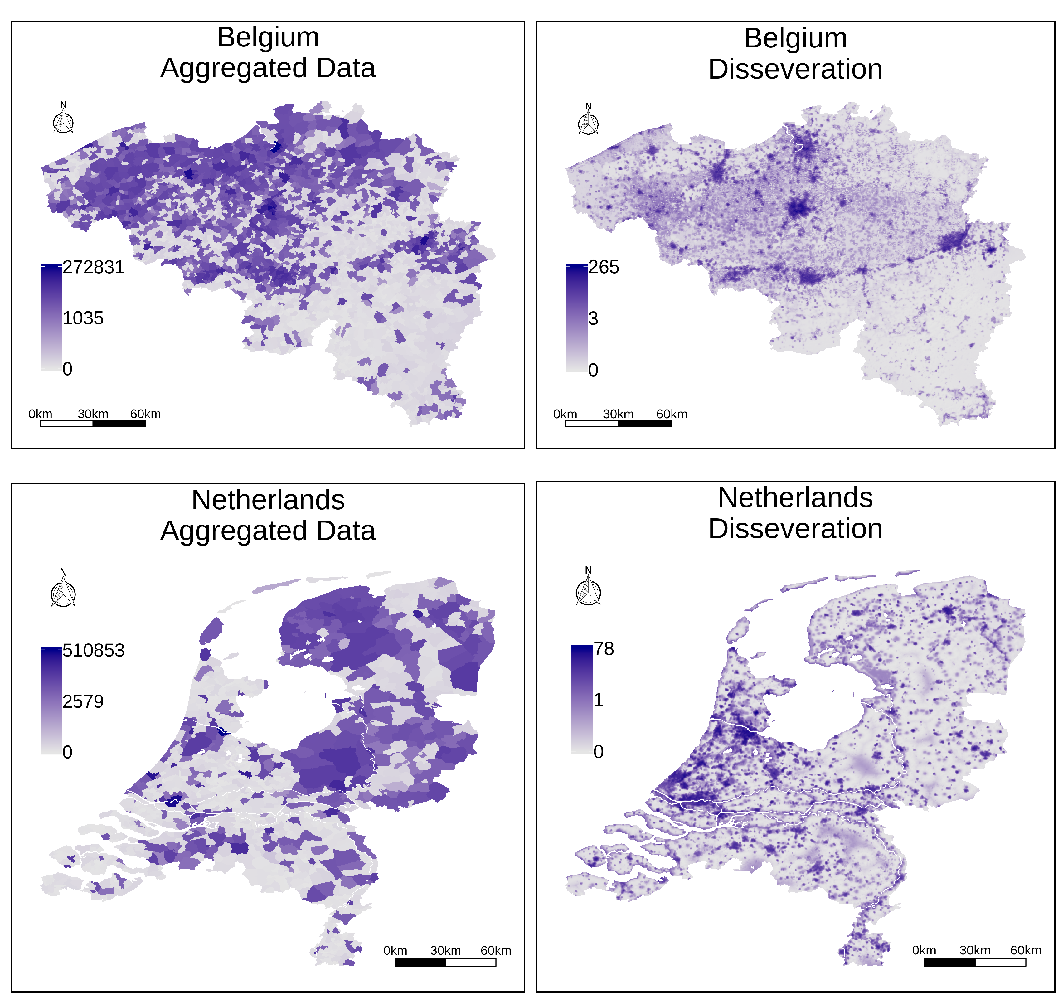
For testing the proposed disaggregation procedure, we started by using the census information at the lowest level of data aggregation that is available (i.e., parishes for Great Britain, and municipalities for Belgium and for the Netherlands), producing raster datasets with a resolution of 200 m per cell. The left part of Figure 5 presents two choropleth maps illustrating the aggregated information at the level of municipalities, for the territories of Belgium and the Netherlands, while the right part of Figure 5 presents the results of the complete disaggregation procedure, leveraging regression analysis based on a convolutional neural network with all sources of ancillary information. All the maps from Figure 5 used a logarithmic transformation to assign data values to particular colors, given that the population counts have a highly skewed distribution in their values.

The maps from Figure 5 illustrate general trends in the resulting distribution for the disaggregated values. Higher values are assigned to coastal regions, large cities such as Brussels or Amsterdam end up receiving a significant proportion of the disaggregated population, and other similar patterns can be observed in the results. For instance, in the northern half of Belgium, the disaggregated population counts are clearly concentrated around the important port of Antwerp, the city of Ghent, and the capital, Brussels. In the southern half, we have a number of smaller towns and cities along the valley of the Sambre and Meuse rivers, where the sillon industriel (i.e., the industrial valley) became a focus of industrialization. In southeast Belgium, along the border with Luxembourg and Prussia, we have the heavily forested and agricultural region known as the Ardennes, with much lower population counts. Interestingly, according to the census data, 1900s Belgium had more people than the Netherlands.

Figure 6 details the disaggregation results for the British census from 1900, focusing on the city of London and its outskirts. We plot, side-by-side, historical land coverage information from the HILDA dataset, modern information on human settlements, modern population density, a satellite photo collected from Google Earth for the same region, the estimates obtained with a baseline disaggregation method corresponding to a proportional and weighted areal interpolation procedure that only used modern population density (i.e., raster $T^d$ from the enumeration shown in Section 3), and the estimates computed with the complete hybrid method leveraging CNNs and all sources of ancillary information. From the figure, and as expected, one can see that more developed areas have higher values, while less developed areas end up with lower values. The historical population density also seems to have a high relation with the modern information given in the GHS datasets, in terms of the geographic distribution of the data.

When further investigating the correlations between the historical population counts and the ancillary variables, we found that there is a very strong linear correlation between the population counts for each aggregation area (e.g., for each parish/municipality) and the aggregated values for some of the different variables that were considered, particularly with the information on modern population density. Consequently, a very high linear correlation is also found for the disaggregated results produced through the dasymetric procedure that relied exclusively on modern population density as ancillary information (i.e., proportional and weighted areal interpolation, leveraging the population counts, constitutes a very strong baseline).

Figure 7 presents two correlation matrices, illustrating the correlations between the ancillary variables that were considered in our study and the historical population counts for Great Britain and Belgium (similar results were observed for the case of the Netherlands). The ancillary variables were aggregated to the level of parish/municipality, in order to compare the values against the historical population counts. For each pair of variables we present also the actual value that was obtained for the Pearson correlation coefficient between the variables, and also an indication for whether the correlation was statistically significant (i.e., three stars corresponds to a p-value of zero, two stars to a p-value of $0.001$, one star to $0.01$, and a single dot to $0.05$).

From Figure 7, one can confirm the relevance of some of the auxiliary variables for the spatial disaggregation of historical population. For instance, one can see (i.e., either through visual observation, or through the computed values for the Pearson correlation coefficient) that the relationship between the ancillary raster corresponding to modern population density and the considered target variables is indeed very strong. The information on modern terrain development and human settlements (i.e., two variables that seem to capture more or less the same information) is moderately correlated with the target variables, and the information on historical land coverage has notably less relevance in the distribution of the target population counts. The regression algorithms should consider parameters based on the importance of such correlations, for instance giving more relevance to the ancillary information provided by the modern population density.

The typical strategy for quantitatively evaluating the accuracy of spatial disaggregation procedures involves aggregating the target zone estimates to either the source or some intermediary zones, and then compare the aggregated estimates against the original counts. Although other evaluation procedures could provide alternative, or even more detailed, information about the quality of the disaggregation methods (e.g., compare the results obtained for administrative divisions with an area smaller than the target resolution of 200 m per cell, with population counts collected from other historical records, in order to exactly capture differences at the target resolution), these would require the availability of data that can be very difficult to collect, and that would likely only be possible to obtain for a small number of regions. With the strategy based on intermediary aggregation zones, the results for the comparison can be summarized by various statistics that capture the quality of the disaggregation results, such as the root mean square error (RMSE) between estimated and observed values, or the mean absolute error (MAE). The corresponding formulas are as follows.

$$\mathrm{RMSE}=\sqrt{\frac{{\sum }_{i=1}^n{({\widehat{y}}_i-y_i)}^2}{n}}$$

(2)

$$\mathrm{MAE}=\frac{{\sum }_{i=1}^n|{\widehat{y}}_i-y_i|}{n}$$

(3)

In Equations (2) and (3), ${\widehat{y}}_i$ corresponds to a predicted value, $y_i$ corresponds to a true value, and n is the number of predictions. Using multiple error metrics can have advantages, given that individual measures condense a large number of data into a single value, thus only providing one projection of the model errors that emphasizes a certain performance aspect. For instance, Willmott and Matsuura [58] proved that the RMSE is not equivalent to the MAE, and that one cannot easily derive the MAE value from the RMSE (and vice versa). While the MAE gives the same weight to all errors, the RMSE penalizes variance, as it gives errors with larger absolute values more weight than errors with smaller absolute values. When both metrics are calculated, the RMSE is by definition never smaller than the MAE. Chai and Draxler [59] argued that the MAE is suitable to describe uniformly distributed errors, but because model errors are likely to have a normal distribution rather than a uniform distribution, the RMSE is often a better metric to present than the MAE. Multiple metrics can provide a better picture of error distribution and thus, in our study, we present results in terms of the MAE and RMSE metrics. We also report results in terms of the normalized root mean square error (NRMSE) and the normalized mean absolute error (NMAE), in which we divide the values of the RMSE and MAE by the amplitude of the true values (i.e., the subtraction of the maximum by the minimum true values). This normalization can facilitate the comparison of results across variables.

To get some idea on the errors that are involved in the proposed spatial disaggregation procedure, we experimented with the disaggregation of data originally reported at the level of larger territorial divisions (i.e., at the level of counties or administrative districts) to the raster level, later aggregating the estimates to the level of parishes/municipalities (i.e., taking the sum of the values from all raster cells associated to each parish/municipality) and comparing the aggregated estimates against the values that were originally available in the census datasets.

Table 1. Results obtained with different disaggregation methods.

	Netherlands
	RMSE	MAE	NRMSE	NMAE
Mass-preserving areal weighting	19,756.9	4176.1	0.0387	0.0082
Pycnophylactic interpolation	19,756.4	4178.8	0.0387	0.0082
Weighted areal interpolation (WA)	17,124.5	3248.2	0.0335	0.0063
Linear regression	17,286.7	3073.7	0.0339	0.0060
Cubist	17,980.9	3394.7	0.0352	0.0066
Gradient boosting	16,989.0	3003.2	0.0333	0.0059
Convolutional neural network	17,484.4	3216.3	0.0342	0.0063
	Belgium
	RMSE	MAE	NRMSE	NMAE
Mass-preserving areal weighting	8690.0	2048.2	0.0319	0.0075
Pycnophylactic interpolation	8660.1	2028.7	0.0317	0.0074
Weighted areal interpolation (WA)	6787.9	1462.1	0.0249	0.0054
Linear regression	6792.2	1459.7	0.0249	0.0054
Cubist	6930.8	1329.8	0.0254	0.0049
Gradient boosting	6518.4	1198.1	0.0239	0.0044
Convolutional neural network	6312.7	1224.5	0.0231	0.0045
	Great Britain
	RMSE	MAE	NRMSE	NMAE
Mass-preserving areal weighting	6271.9	1418.2	0.0197	0.0044
Pycnophylactic interpolation	6034.7	1376.1	0.0189	0.0043
Weighted areal interpolation (WA)	5648.7	1178.9	0.0177	0.0037
Linear regression	5660.6	1162.9	0.0177	0.0036
Cubist	5170.0	1013.0	0.0162	0.0032
Gradient boosting	5255.8	1037.3	0.0165	0.0033
Convolutional neural network	5117.1	1009.8	0.0160	0.0032

shows the obtained results, comparing the disaggregation procedure leveraging different types of regression algorithms, against simpler baselines corresponding to (i) mass-preserving areal weighing, (ii) pycnophylactic interpolation, or with (iii) weighted areal disaggregation leveraging population data for the weights (i.e., raster $T^d$ in the enumeration given in Section 3). Values in bold correspond to the best results for each variable.

The results from Table 1 show that the hybrid method outperforms the baselines corresponding to mass-preserving areal weighting or pycnophylactic interpolation. However, the simpler dasymetric procedure that only uses modern population density as ancillary data produces results that are quite similar to those achieved by the methods that leverage regression analysis, in some cases (e.g., in the case of testes using linear regression) even slightly superior.

To some degree, the strong linear dependence between modern population density and the historical population can explain why the relatively simple weighted areal disaggregation method, or why the approach based on linear regression, can achieve results that are almost as good as the more sophisticated methods. However, the obtained results also showed that approaches based on more advanced procedures for regression analysis (e.g., convolutional neural networks or gradient tree boosting) achieved the best results overall. It should also be noted that the errors that were reported correspond to an upper bound on the actual errors produced from the disaggregation of data reported at the level of parishes/municipalities (i.e., we only measured the errors in the disaggregation of data originally at the level larger territorial divisions), given that, in principle, the higher the differences between the source and target areas, the higher the errors introduced by a disaggregation procedure.

The best results for Great Britain were obtained with Convolutional Neural Networks (CNNs), while gradient boosting achieved the best results for the Netherlands. Mixed results were obtained for Belgium, with CNNs obtaining better values for RMSE. While we have no definitive explanation for these differences, we noticed that the weighted areal disaggregation method has a much higher correlation towards the historical population counts in the case of Great Britain. This can be seen in the plots from Figure 7, which compare Great Britain to Belgium (in the case of the Netherlands, the results are similar to those obtained for Belgium, e.g., with a correlation of 0.52 between the historical population counts and the results of weighted areal disaggregation). The results from the weighted areal disaggregation are used in the first step of the hybrid procedure, as inputs to the learning algorithms. The CNN approach is perhaps better at capturing the patterns originally present in the results from the weighted areal interpolation.

In an additional set of experiments, we tried to assess the degree to which the different ancillary variables contribute to the final disaggregation results.

Table 2. Results obtained with different sets of ancillary variables.

Netherlands	Linear Regression				Convolutional Network
	RMSE	MAE	NRMSE	NMAE	RMSE	MAE	NRMSE	NMAE
Historical data	19,692.8	4232.9	0.0386	0.0083	18,771.8	4301.8	0.0368	0.0084
Historical +WA	17,221.0	3089.3	0.0337	0.0060	17,263.3	3084.6	0.0338	0.0060
Modern data	17,412.5	3207.0	0.0341	0.0063	17,525.3	3333.0	0.0343	0.0065
All variables	17,286.7	3073.7	0.0339	0.0060	17,484.4	3216.3	0.0342	0.0063
Belgium	Linear Regression				Convolutional Network
	RMSE	MAE	NRMSE	NMAE	RMSE	MAE	NRMSE	NMAE
Historical data	8573.5	2059.8	0.0314	0.0076	8138.0	2285.2	0.0298	0.0084
Historical +WA	6792.0	1460.4	0.0249	0.0053	6413.8	1227.4	0.0235	0.0045
Modern data	6809.7	1342.0	0.0250	0.0049	6557.4	1208.1	0.0240	0.0044
All variables	6792.2	1459.7	0.0249	0.0054	6312.7	1224.5	0.0231	0.0045
Great Britain	Linear Regression				Convolutional Network
	RMSE	MAE	NRMSE	NMAE	RMSE	MAE	NRMSE	NMAE
Historical data	5933.4	1398.1	0.0186	0.0044	5773.1	1263.9	0.0181	0.0040
Historical +WA	5662.4	1222.6	0.0177	0.0038	5447.3	1087.7	0.0171	0.0034
Modern data	5665.5	1180.5	0.0178	0.0037	5270.4	1024.1	0.0165	0.0032
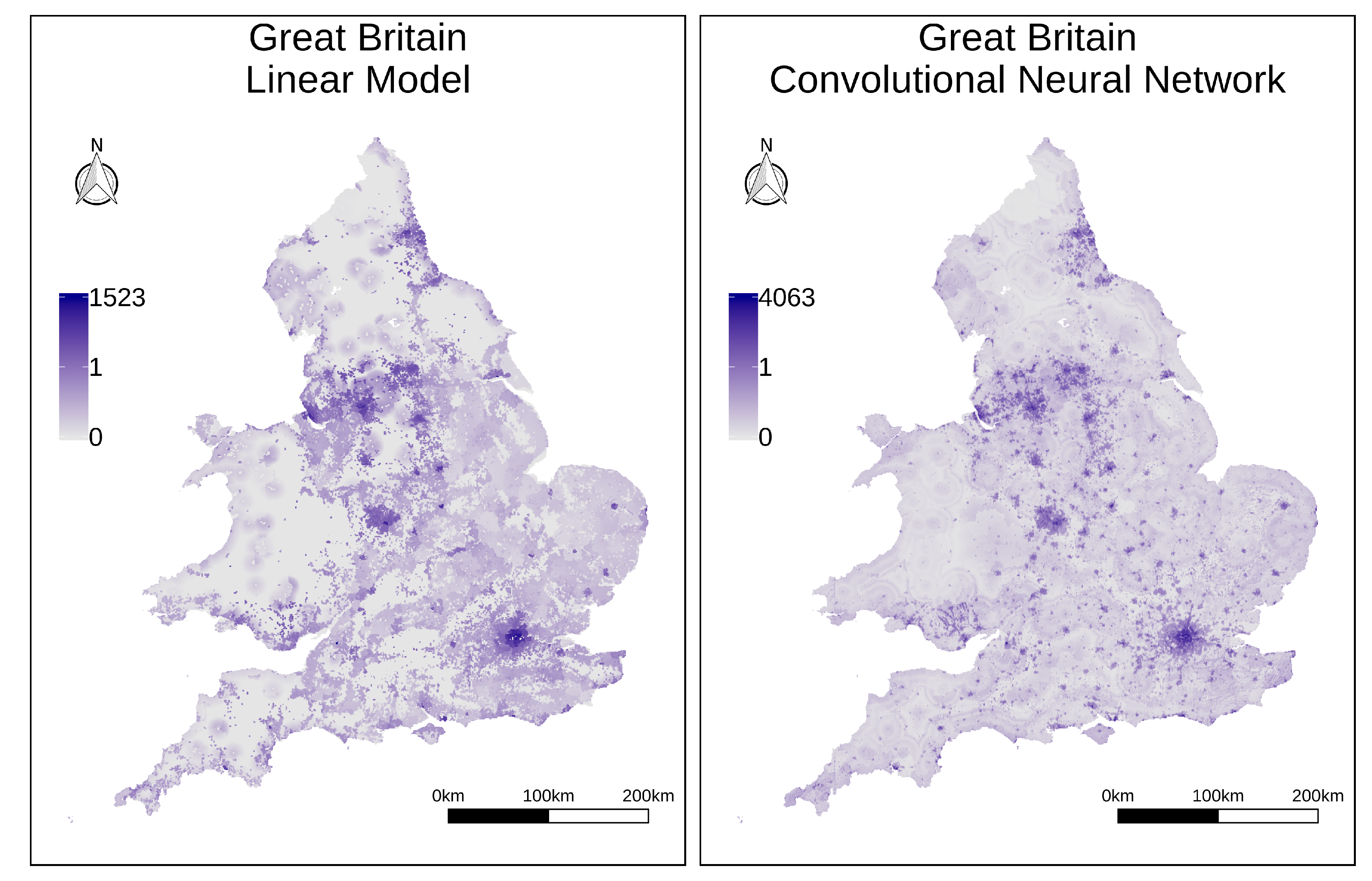
All variables	5660.6	1162.9	0.0177	0.0036	5134.9	1009.5	0.0161	0.0032

reports on the results of experiments with different sets of ancillary variables, considering both linear regression analysis, or regression based on the convolutional neural network. Moreover, Figure 8 presents maps for the disaggregated historical population of the territory of Great Britain, respectively considering the worst (i.e., linear regression leveraging just the historical variables) and the best model (i.e., a convolutional neural network with all the ancillary variables) from Table 2. The results confirm that all the considered variables, including the variables reporting modern/contemporary information, seem to contribute to improving the disaggregation results. Nonetheless, simpler models with fewer variables remain quite competitive, in some cases (e.g., when using only modern data in the case studies relative to the Belgian and British territories) even superior in some error metrics.

5. Conclusions and Future Work

This article reported on experiments with a hybrid spatial disaggregation technique that combines the ideas of dasymetric mapping and pycnophylactic interpolation, using machine learning methods (e.g., ensembles of decision trees, or deep learning methods based on convolutional neural networks) to combine different types of ancillary data, in order to disaggregate historical census data into a 200 m resolution grid. We specifically present results related to the disaggregation of historical census data collected for Great Britain, Belgium, and the Netherlands, which indicate that the proposed method is indeed highly accurate, outperforming simpler disaggregation schemes based on mass-preserving areal weighting or pycnophylactic interpolation.

Despite the interesting results, there are also many open challenges for future work. Our experimental results indicate that regression modeling based on CNNs leads to interesting results, although we have only experimented with a relatively simple neural network architecture. In the future, we plan to also evaluate the proposed approach with data for smaller regions (i.e., compatible with the target resolution of 200 m per cell) having known values in terms of historical population, this way obtaining different estimates for result quality (i.e., errors measured directly at the target resolution). We also plan to experiment with different types of model ensembles (e.g., ensembling CNN results), this way perhaps improving the quality of the obtained results and, at the same time, allowing us to estimate the disaggregation quality at the level of individual cells (i.e., the variance in the results from the different models in the ensemble can be used to estimate the certainty of the predictions for a given cell). Moreover, we plan to experiment with more advanced CNN architectures [23,52,60,61], similar to those that are currently achieving state-of-the-art results in different types of image processing and computer vision problems (e.g., in tasks such as aerial image segmentation [62] or image super-resolution [63]).

The experiments that are reported on in the present article have also been limited to the disaggregation of historical census data referring to specific individual years, although it could be interesting to consider temporal interpolation, in order to infer disaggregated population counts for the years in between census collection. Similar methods to those used in the present study can, in principle, be adapted to simultaneously perform population disaggregation and population projection to different years, taking inspiration on recent experiments with modern data [41].

Finally, in terms of future work and taking inspiration on recent studies within the realm of the spatial humanities, we also plan to experiment with the inclusion of other types of ancillary variables (e.g., proximity towards the historical transportation network [19,20,21], or information on building footprints obtained from the segmentation of historical maps [64]), and with other types of spatial disaggregation tasks that involve historical datasets (e.g., disaggregation of indicators relative to health problems [65,66,67,68,69] or historical tourism [70,71]), leveraging ancillary data collected from textual sources through the application of geographical text analysis. Although the present study focused on the disaggregation of population counts, the proposed methods can naturally also be applied in the disaggregation of socio-economic indicators relevant for different types of historical inquiries.