1. Introduction
Time-series analysis and pattern detection are important knowledge-discovery tasks [
1]. Time-series analysis is widely used in future forecast and control changes [
2], such as investigating transport demands corresponding to economic growth or gasoline prices from decade-based historical data [
3,
4,
5], monitoring and measuring the displacement of Earth’s surface or deforestation [
6,
7], or understanding the mobile traffic of large-scale cellular networks [
8]. Time-series clustering is a time-series analysis method and a special type of clustering. Time-series clustering has been widely used in mining clustering distributions of a time series. In such a process, the time series are grouped based on a certain similarity measure [
9]. The technique of dynamic time warping (DTW) is proposed to measure the distance between time series. While first introduced and explored to apply in the area of speech recognition [
10], the DTW algorithm is now used in many areas, including handwriting and signature recognition [
11,
12], network-traffic monitoring [
13], human-gesture recognition [
14], and protein-sequence alignment [
15].
Time-series data are widely used in domains that involve temporal measurements. There are two typical time-series data in the transportation field, the trajectory data that represent the mobility of moving objects [
16], and a monitoring log in a fixed area, such as traffic-flow data for a road section collected by a fixed sensor, or the passenger flow of a metro station in over prolonged period. In trajectory data, each element of the time series represents a spatial point with a corresponding timestamp, usually collected by a Global Positioning System (GPS) device. With the wide spread of monitors and automated fare-collection systems, public-transport operators have collected a mass of user-transaction data. User-generated data can be transferred to time series, which provide the operators and planners with opportunities to learn about the behaviors and travel patterns of transit users [
17].
Bike-sharing systems (BSSs) based on GPS- and Internet-enabled devices have become popular transportation infrastructures in cities in recent years. These systems are useful complements to traditional public-transport services. It is necessary to comprehend the spatial–temporal characteristics of BSS travel demands to optimize the operation and reduce the waste of bike and human resources. Zhou, X. [
18] investigated the spatiotemporal biking patterns in Chicago by analyzing docked BSS data. Positions of bike check-in and check-out are discretized in docked BSS, while additional spatial discretizing steps are needed when analyzing dockless BSS data. This study uses a grid-based method to discretize spatially continuous dockless BSS data. Another difference between docked and dockless BSSs is that dock capacities are limited, which could influence check-in and check-out behaviours of riders. For example, people may give up using shared bikes because of empty docks or adjust their check-in positions because of full docks, causing the problem of overdemand. Capacities are more flexible in dockless systems.
Some motivation mechanisms could be applied to encourage normal bike users to participate in the operation of a bike-sharing system, for example, ‘bonus bikes’. Users can get some rewards after riding a bonus bike, usually from and to specific areas. This mechanism can help reduce the accumulation of bikes in some areas.
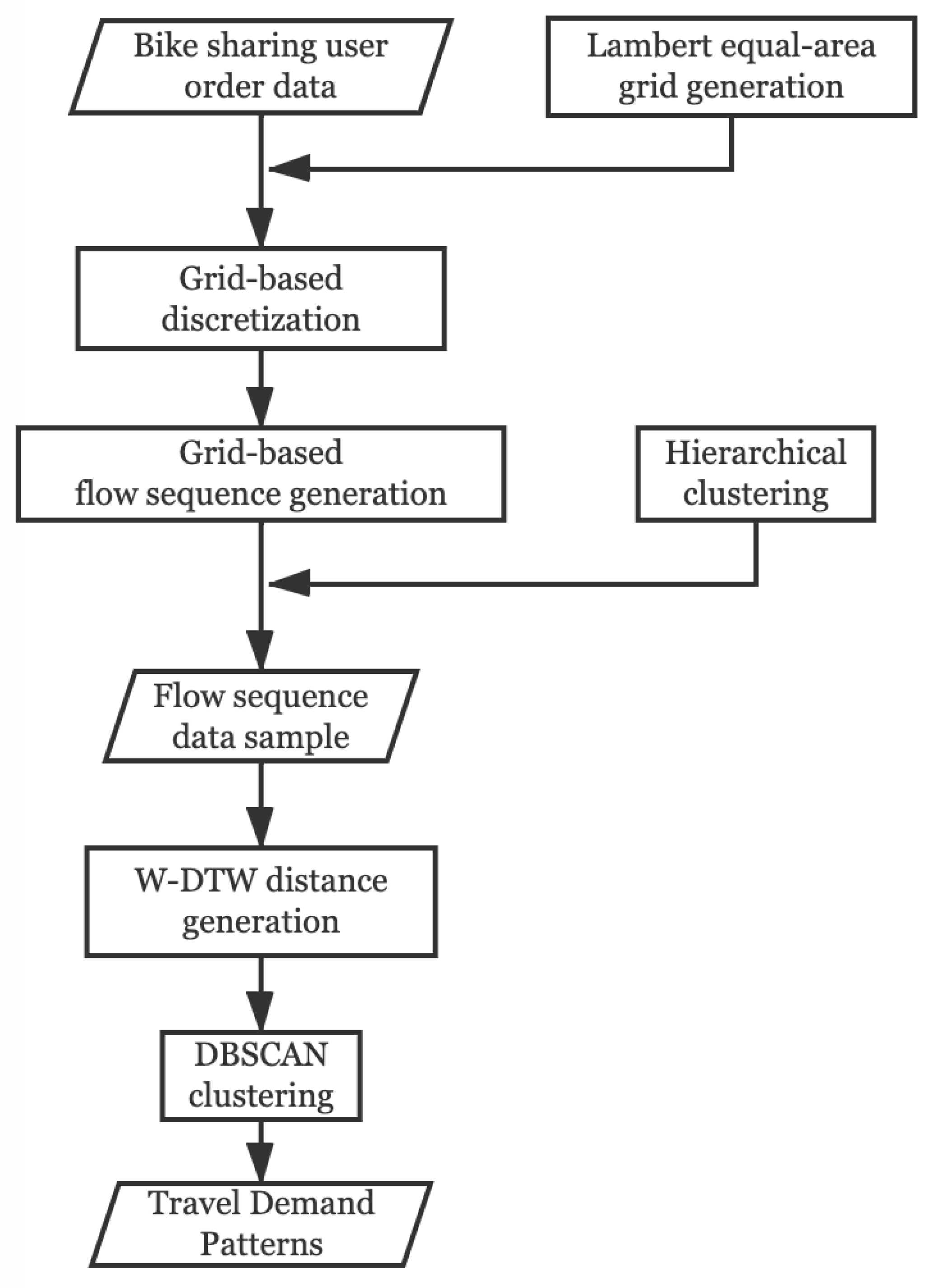
This study aims to develop a data-processing model that converts spatiotemporal-point datasets into temporal sequences using a grid-based method and time-series data-mining technologies to uncover the patterns and regularities of travel demands from data. This study uses a Lambert equal-area grid to discretize the bike-sharing-system data into grids; then, travel demands in different city areas are modeled as time-series data (i.e., flow sequences) in each grid cell. The time-series data-analysis methods of dynamic time warping and density-based spatial clustering of applications with noise (DBSCAN) were applied to find the typical travel-demand patterns in travel-demand data samples following
Figure 1.
2. Data and Study Area
We used BSS historical-order data in Beijing produced by the Beijing Mobike Technology Co., Ltd. (Beijing, China), the owner and operator of the Mobike bicycle-sharing system. Mobike bicycles are equipped with GPS- and cellular-enabled smart locks, allowing the operator to collect exact positions of lock and unlock events. The user ID, bike ID, unlock/lock time, unlock/lock location, and total cycling distance of every transaction in the Mobike BSS are recorded. These data were imported into a spatially enabled PostgreSQL object-relational database with a PostGIS extension, where the coordinate values were converted into spatially referenced geometries. Among the one-month user order data (October 2017) consists of 70.6 million orders, a total of 5.08 million individual users and 0.97 million bicycles were identified. Considering the cost of computations, we used data from 23 October, Monday, to 27 October 2017, Friday, in the following data-mining processes.
The fields of the BSS order data are UserID, OrderID, BikeID, StartTime, StartPosition, EndTime, EndPosition, TotalDistance, Gender, Age, RegCity (city code where the user registered). Each record in the user order dataset could be modeled as two spatiotemporal events: Unlocking (origin of the trip) and locking (destination of the trip), with spatial locations and corresponding timestamps.
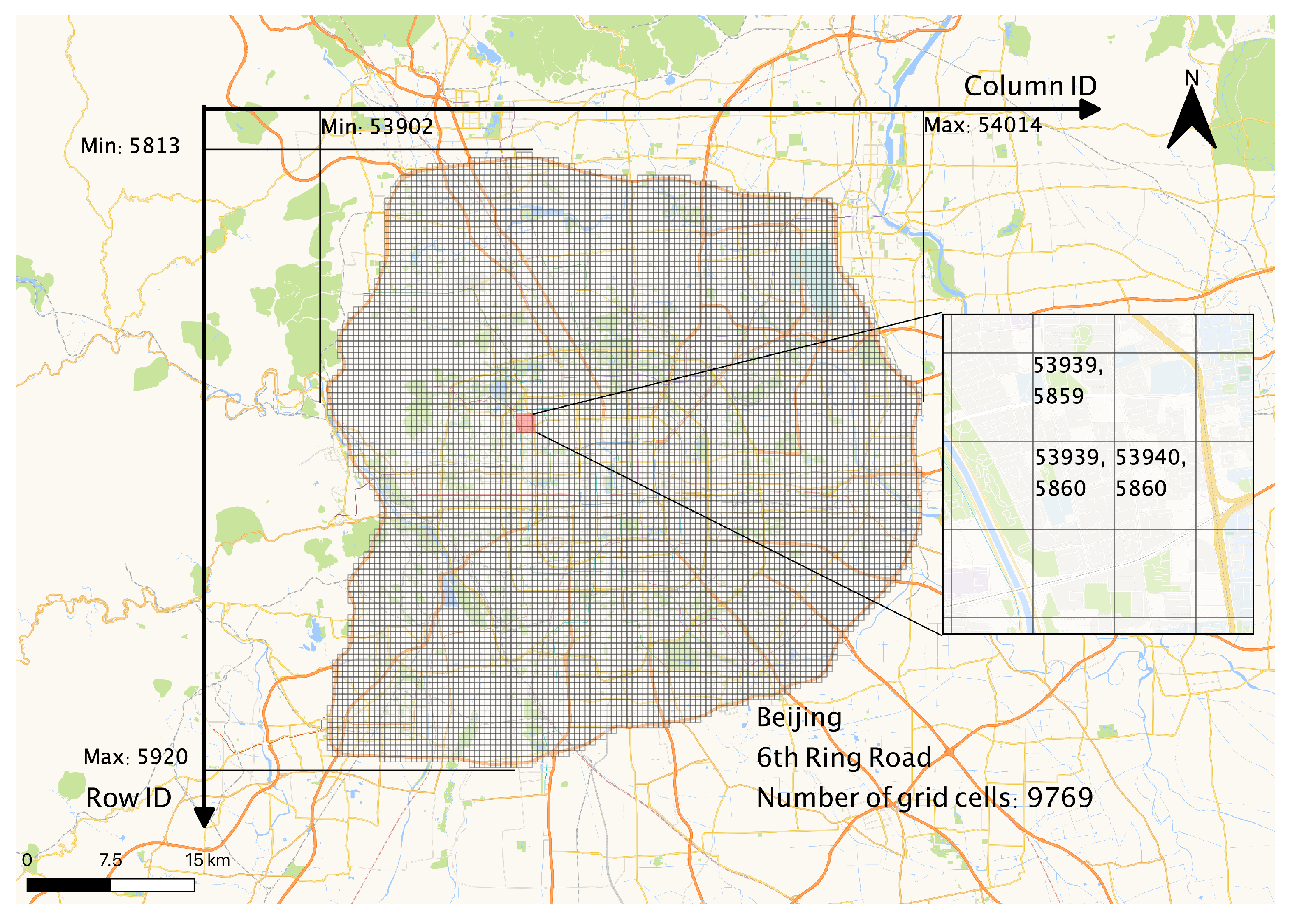
The study area was the district inside the sixth Ring Road of Beijing, as shown in
Figure 2 (The algorithm to generating the grid and grid-cell-numbering schema is introduced in
Section 3.1), which covers several large commuting areas, most bus stops, almost all metro stations, and all major transportation hubs.
3. Methodology
3.1. Spatial Discretization: Generation of Lambert Equal-Area Grid
The grid-based method was applied to measure travel demand of the bicycle -sharing system. With a grid covering the study area, every unlocking and locking event was allocated a grid cell. Once the order records are allocated, the total number of trip-start and trip-end events could be calculated, as well as the bicycle inflow, outflow, and net flow sequence of each grid cell.
The spatial reference system of the original data was WGS-84, in which each spatial point is represented as latitudes and longitudes. To count the number of unlocking/locking events in each grid cell, a projection method that makes little area distortion need to be applied. All map projections necessarily create some distortion of shapes, distances, or areas [
19]. The grids of this study were created using Lambert cylindrical equal-area projection, which minimizes differences in areas between grid cells on the true three-dimensional spheroid.
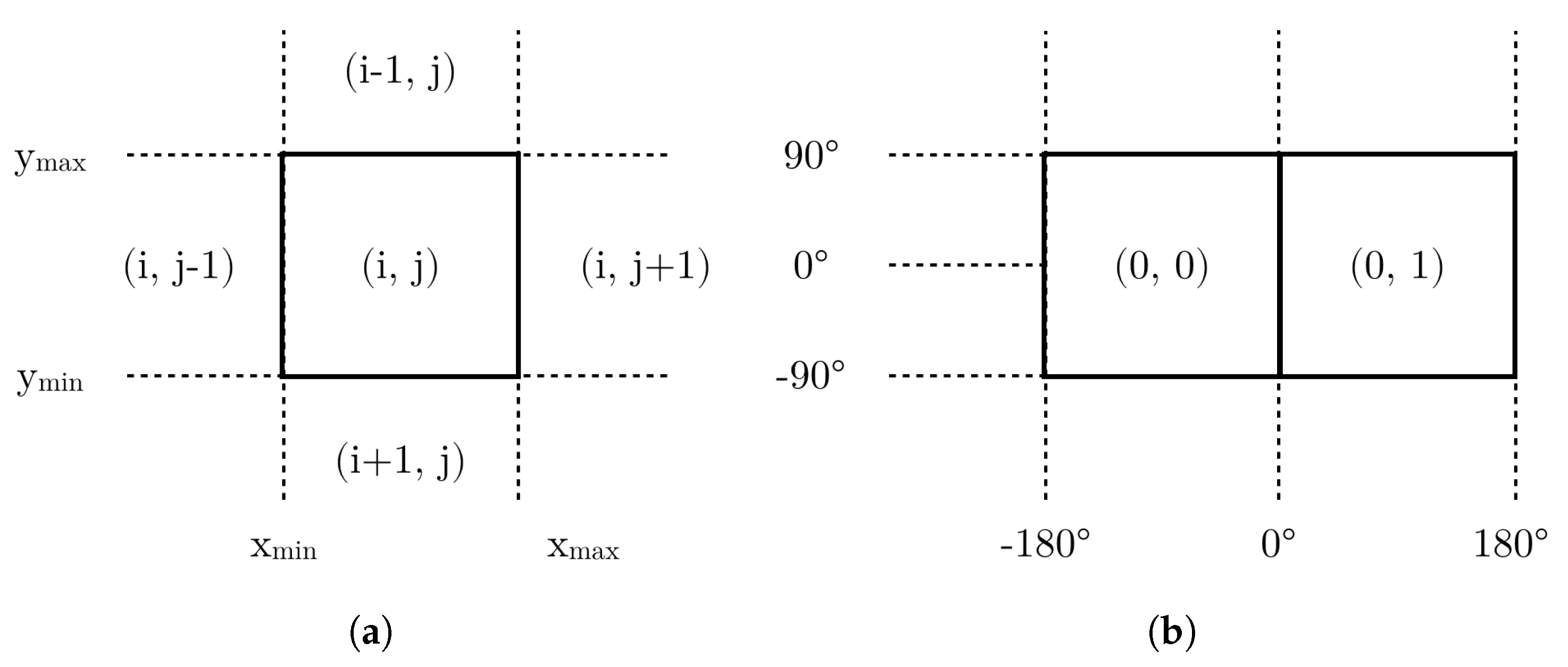
Assuming that the entire globe (180° W–180° E, 90° S–90° N) is covered by two cells at zoom level 0 (
Figure 3b), each level 0 cell can be divided into four level 1 cells using the quadtree method. Every level
l grid cell can be divided into four level
grid cells.
The numbering schema of the Lambert equal-area grid is continuous for each level, as shown in
Figure 3a. The grid cell in the northwestern corner has (row ID, column ID) =
. With a given zoom level
and (row ID, column ID), a Lambert grid cell can be created using Equation (
1).
where
i and
j are the row ID and column ID of the grid cell, and
are the longitudes or latitudes of the boundaries of each cell as shown in
Figure 3a.
The cell size of the grid should be small enough to indicate the spatial differences of demands between different areas in Beijing, and large enough for statistical significance and acceptable computational cost. We assume that the service radius of BSS is close to the average five-minute walking distance of adults, that is, 402 m [
20]. In addition, the cell size should be smaller than most cycling distances in order to identify the origin-destinations of individual trips.
In this study, we created a level-15 Lambert equal-area grid (as shown in
Figure 2) whose cell size was approximately
. The number of cells covering the study area was 9769, among which the difference in area (on the true three-dimensional spheroid) caused by projection distortion between the largest and the smallest cells was less than 0.013%, which is negligible in this study.
Given any position
under the WGS-84 reference system and the level of tge Lambert grid, the (row ID, column ID) of the grid cell to which
P belongs can be calculated by Algorithm 1. Algorithm 1 can be derived from Equation (
1). We compute the grid ID for each lock/unlock event in advance, then build indices on these IDs and count the number of lock/unlock events in each grid cell.
| Algorithm 1 Calculate grid ID of given position in Lambert equal-area grid. |
| Require: |
| Longitude x under WGS-84 reference system; |
| latitude y under WGS-84 reference system; |
| level of Lambert Grid l; |
| Ensure: |
| —Column ID and row ID of the grid cell (as shown in Figure 2) where position P belongs. |
| |
| |
| return |
SQL Procedural Language PL/pgSQL with PostGIS extension support was used to create the grids, to count lock and unlock events that happened in each cell, and to calculate the indices of each cell. With the spatial discretization method proposed in this section, many spatiotemporal datasets, e.g., social-network check-in datasets and mobile-network signaling datasets, can be discretized for further analysis.
3.2. Temporal Discretization: Generation of Travel-Demand Sequence
To generate the inflow, outflow, and net flow sequence of the grid cells, the timestamps of lock and unlock events were discretized into 1 h intervals. The time index of each event is represented as t. For example, in the five-weekday study period, represents (Monday 23 October 2017, 0:00–1:00), while represents (Friday 27 October 2017, 3:00–0:00).
The number of lock events (i.e., trip end) at time index
t inside a grid cell is regarded as the inflow of the cell, which is represented as
, where
c is the grid ID of the cell. Similarly, the outflow of a grid cell (i.e., the number of trips whose start positions are inside this cell) is represented as
. The net flow per hour of a cell
can be calculated using Equation (
2).
The inflow, outflow, and net flow sequence of each cell , , and were calculated.
The sum of
and
per day is represented by
:
The in/out/net flow-sequence data in the database are shown as
Table 1.
Because of the continuity of the grid cells’ spatial distribution, most cells have few or no user-transaction events.
of the grid cells forms long-tailed distribution. It is not that meaningful to cluster those cells and try to find typical travel-demand patterns from them. A hierarchical clustering strategy is applied to detect potential clusters from the travel-demand sequence dataset. The travel-demand sequences are first clustered based on the scale of cycle flow (i.e.,
) using the Jenks natural-breaks [
21] classification method. With the 9769 samples, the seven detected classes are shown in
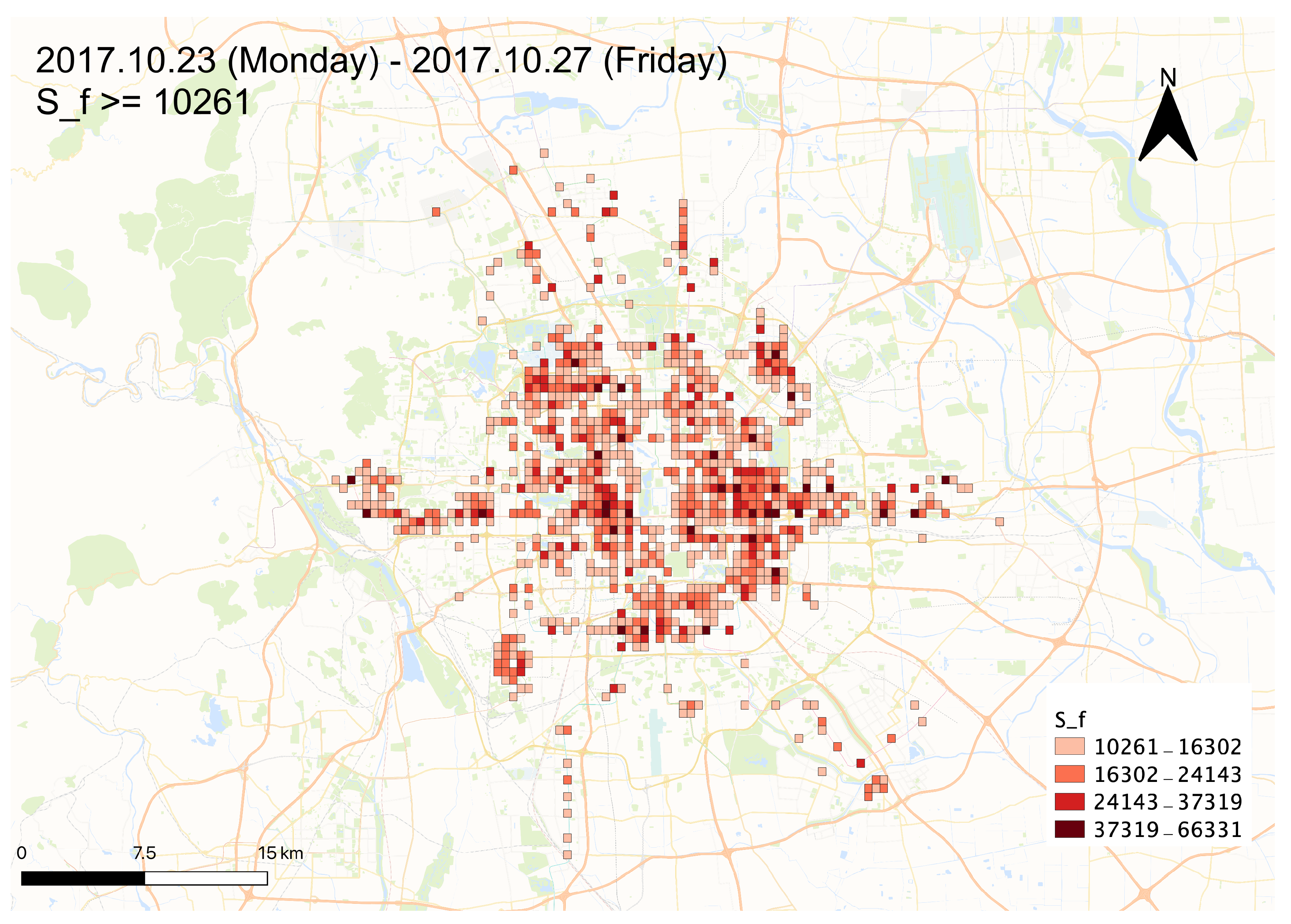
Table 2. The distribution of the 919 grid cells with relatively large
values (
, the 4/5/6/7th bins in
Table 2) are shown in
Figure 4 as a value-by-alpha map [
22]. The following clustering methods were applied to the 919 sample subset.
3.3. Weighted DTW Distance (W-DTW)
The dynamic time-warping algorithm uses a dynamic programming approach to fit the time axis [
1], allowing the more intuitive calculation of distance [
23]. Given two time series
S and
T,
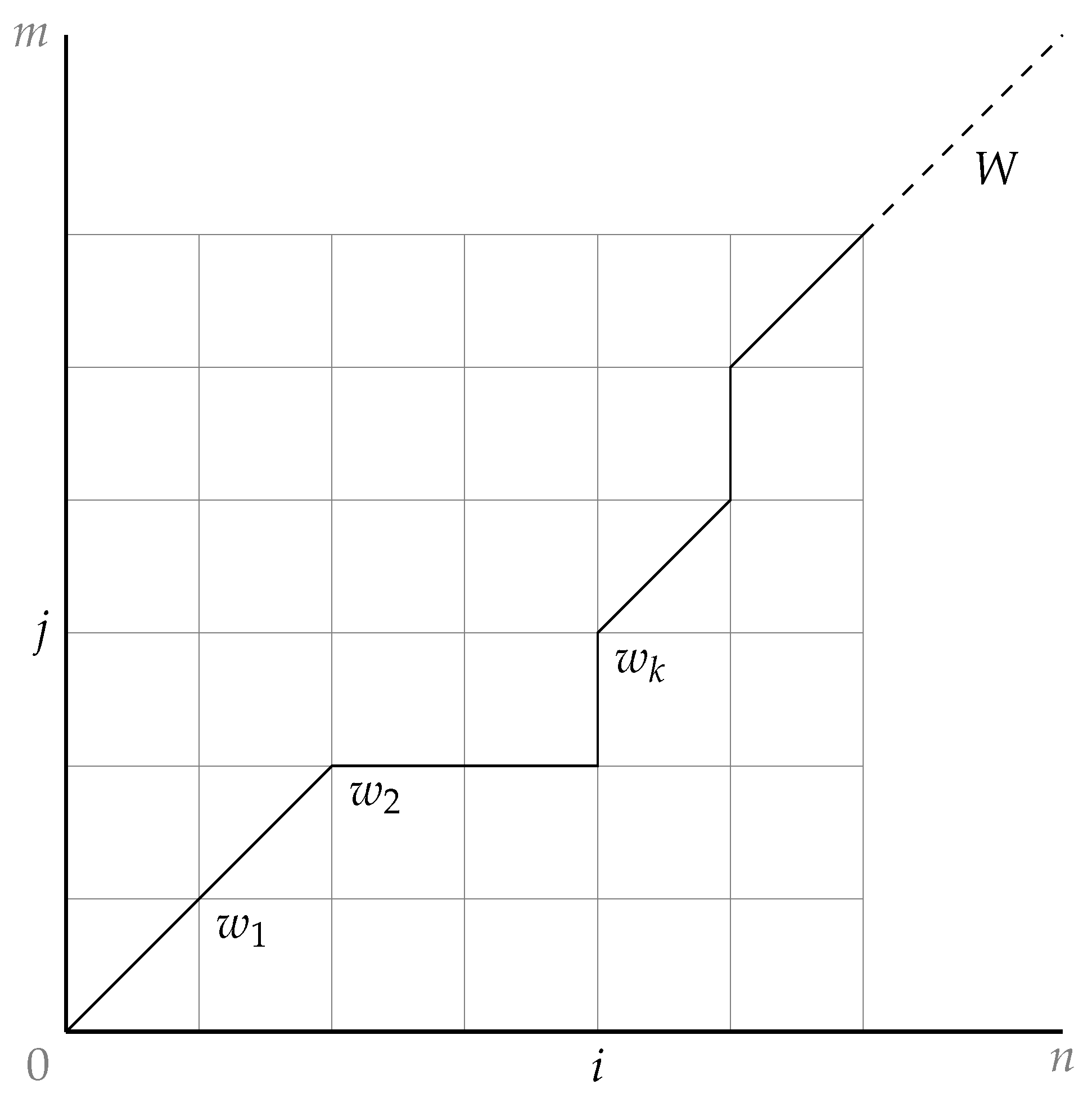
The index of S and T can form an n-by-m grid, where each grid point corresponds to an alignment between elements from sequence S, and from sequence T.
Warping path (
Figure 5)
is a sequence where each
corresponds to a grid point
, such that the distance between
S and
T calculated along warping path
W is minimized. To calculate the cumulative distance between the two series, the distance between two elements
should be defined. For one-dimensional time series, where
and
are scalars,
can be defined as
For high-dimensional data in which
and
are vectors,
can be defined as
where the norm can be calculated as a Euclidean norm for simplicity.
Once the distance measure between the two elements
is defined, the dynamic time-warping problem is defined as a minimization problem, and the target DTW distance can be calculated by Equation (
8).
A dynamic programming approach was applied to find the optimized time-warping path
W. Since the time complexity of the brute-force method of searching and computing all possible warping paths is explosive, and thus unacceptable, some restrictions of search space should be defined [
1]:
Continuity: For every pair of neighboring points and , , and , and
monotonicity: and , and
boundary conditions: The warping path W starts from , and ends at , i.e., , , , .
DTW distance can effectively handle similar time series that are not well-aligned. Since the aim of transportation-usage data analyzed in this study is to detect potential travel-demand patterns, to optimize the operation of bike-sharing systems, the flow direction of rush hours and the balance of grid cells are important, while absolute rush-hour indices can be ignored in some cases. If the net flow of a grid cell is balanced throughout the day, it means that the operator does not need to deliver or dispatch bikes into that grid cell.
Each pairwise distance
in the calculation of DTW distance is treated ’as is’ by default, which means the weight of each pairwise distance is 1.0. Adding weights to each of the pairwise distance allows the distance measure to penalize or favor certain types of point to point correspondence [
10]. In some time-series data-mining-related works, the idea of weighted DTW seems to be valid [
24]. To make peak values more significant, we modified the distance metric to add a weight for the pairwise distance. Using the symmetric weight schema, we obtain Equation (
9).
3.4. Density-Based Clustering for Large-Flow Grid Cells
Density-based cluster method DBSCAN and W-DTW distance are used to cluster bike flow sequences of grid cells to detect typical travel-demand patterns. This study used net flow sequences
of the 919 grid cells with large
as samples to be clustered. The
sequences are first normalized by Equation (
10) before the W-DTW distance matrix is calculated. With the W-DTW distance matrix, the DBSCAN clustering method is deployed to find clusters in the 919 samples.
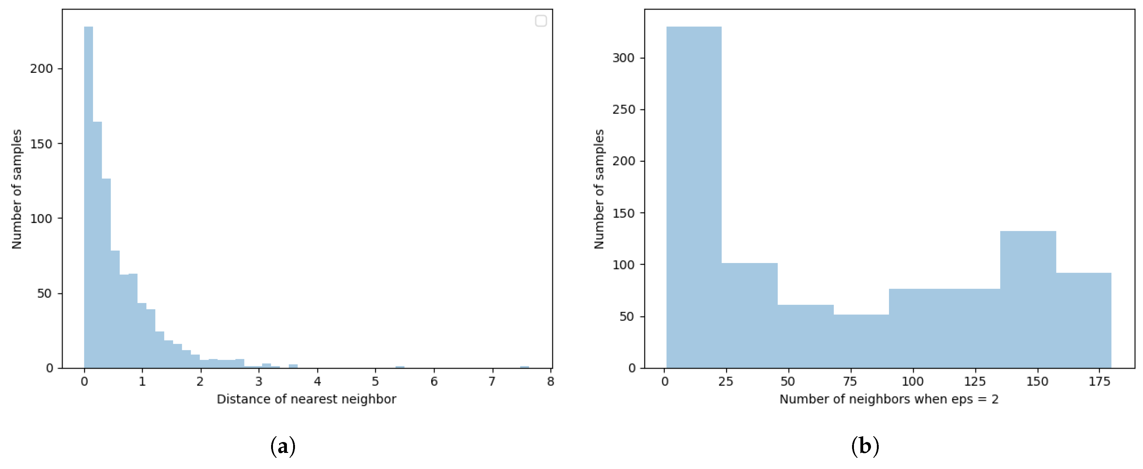
The DBSCAN algorithm requires two parameters, (1) epsilon(
), which specifies the search radius in finding neighbors of points, and (2) MinPts, which determines how many neighbors a point should have to be considered as a core point. With the precomputed W-DTW distance matrix, we calculate the distance to the nearest neighbors of each point. The result is shown in
Figure 6a. The result indicates that most points lie within 2.0 units from their nearest neighbors, so 2.0 is a reasonable guess for parameter
.
We then calculated the number of neighbors of each point within the radius of
, and the result is shown in
Figure 6b. The result indicates that many points (about 320 of 919) have too few neighbors and may be classified as noise. Thus, 25 is a reasonable guess for parameter MinPts.
Since bike-sharing systems are effective complements to traditional public-transport services, a large number of BSS users tend to use bicycles to solve “the last-mile problem”, but take rail transit systems as their main means for commuting. Therefore, subway stations have a significant effect on the spatial distribution of bike-trip generation and attraction. Many heavy-travel demands are generated by commuters, who ride bicycles to go to a subway station from home in the morning, making bicycles overstock around subway stations during the daytime until the evening rush hours.
4. Results and Discussion
Four clusters were detected in the 919 grid cells with a large
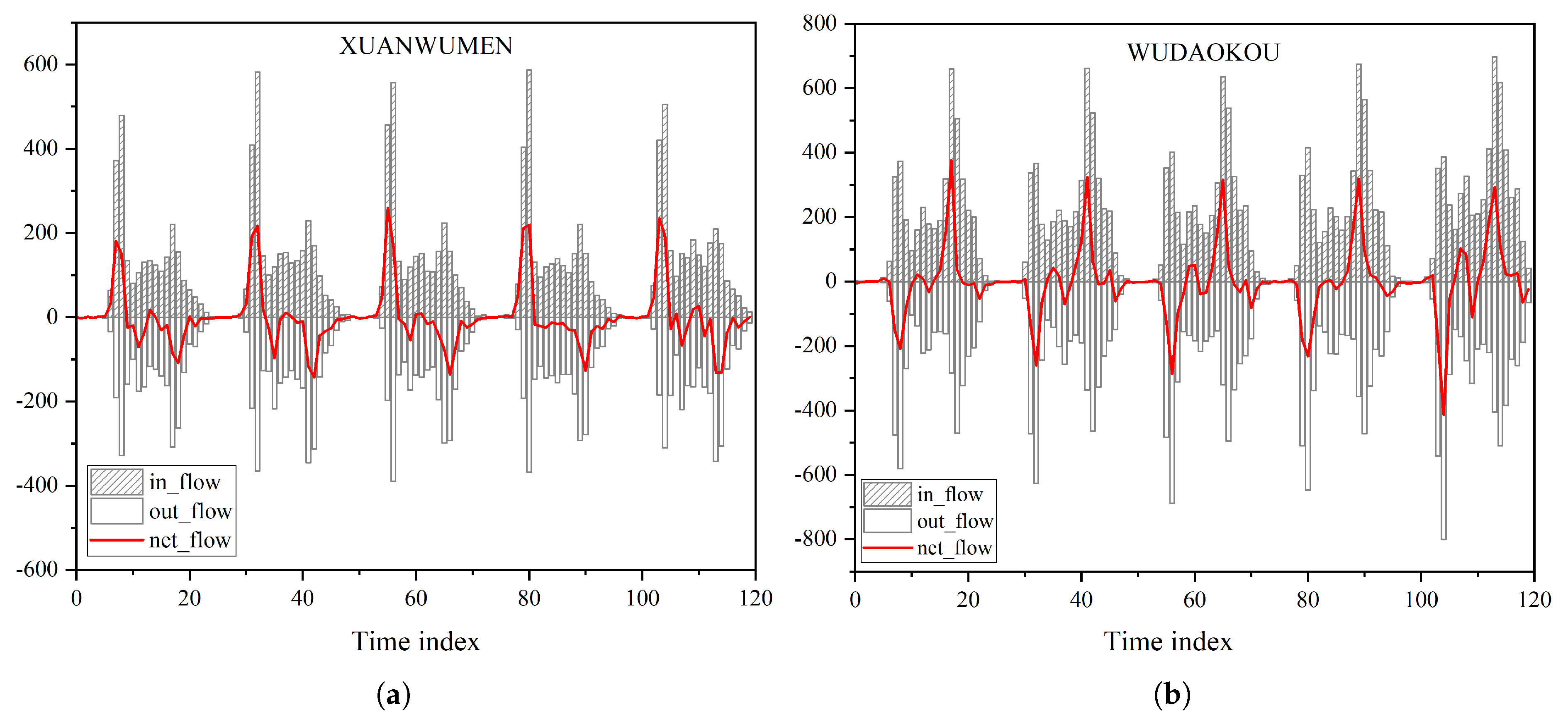
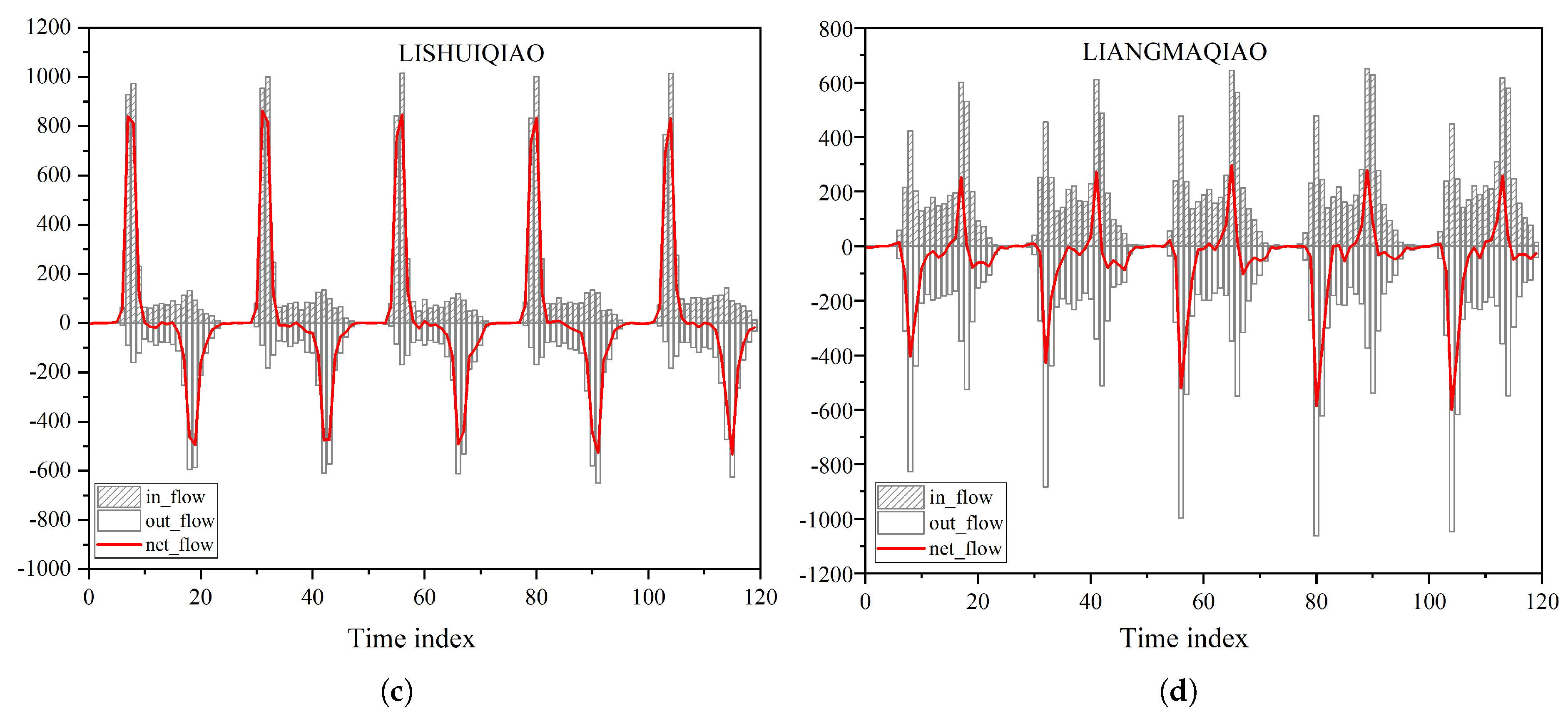
. There were 255 grid cells classified into the four clusters, while the others were regarded as noise because of implicit travel-demand sequence features and/or algorithmic error. Examples of each cluster are shown in
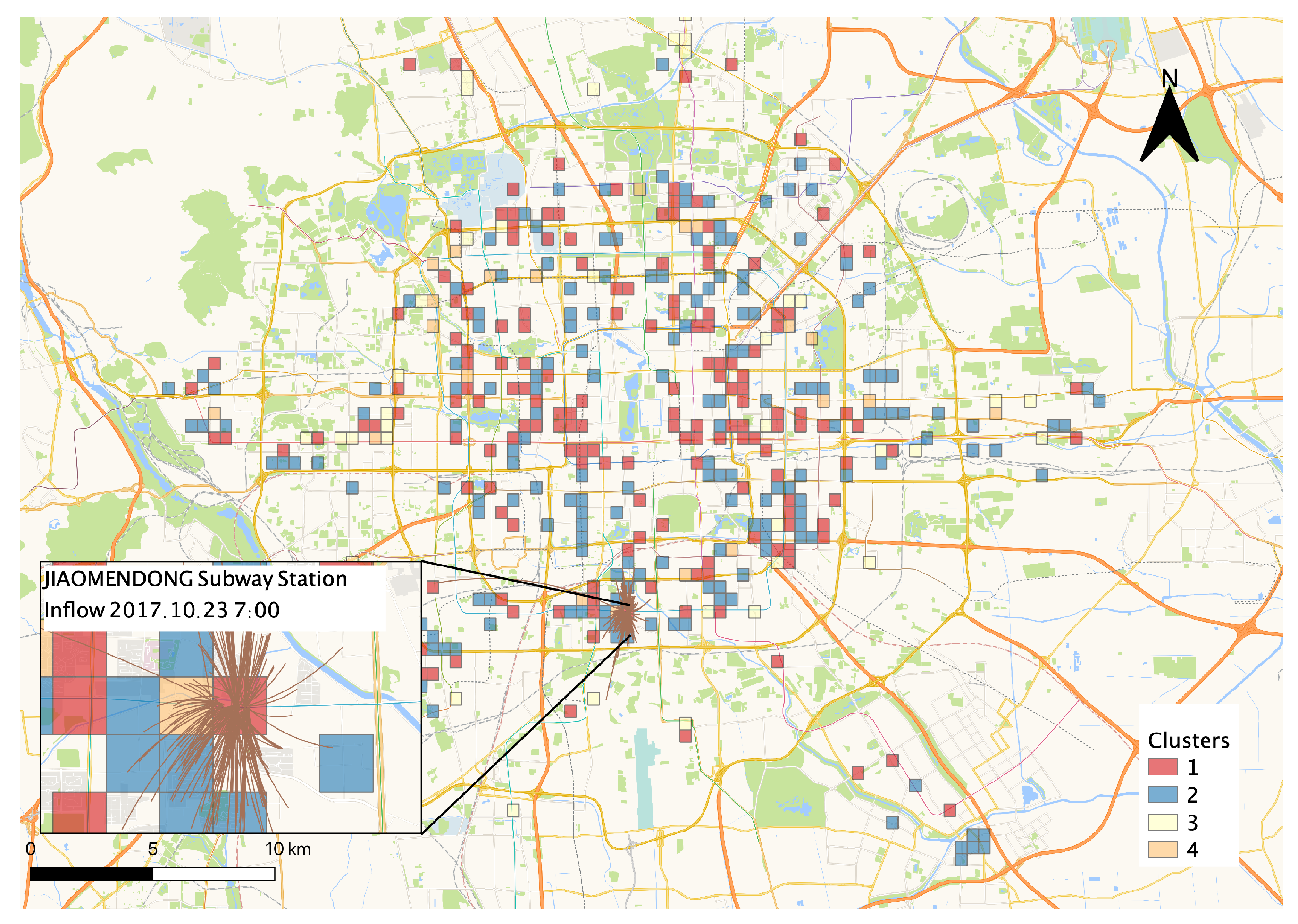
Figure 7, and the spatial distribution of the clusters is shown in
Figure 8.
Grid cells in Cluster 1 shown in
Figure 7a had large inflow in the morning rush hour (7:00–9:00), and massive outflow in the evening rush hour (17:00–20:00). This pattern usually exists near subway stations in a city’s residential areas. Most commuters rent bikes to transfer to urban rail transit. The scales of net flow during the morning and evening rush hours are similar, which means the sum of the net flow sequence throughout the day is relatively small. Thus the number of bikes remains relatively stable over a long period, without manual adjustment by the operator. However, since there are a large number of bikes flowing in the area in the morning that stay used until the evening rush hour, it can be considered a waste of resources. Contrary to the pattern in Cluster 1, demand patterns in Cluster 2, shown in
Figure 7b, have massive outflow in the morning and large inflow in the evening. This flow pattern usually happens near business areas, as commuters use the shared bikes as a transition from subway systems to places of work. Similar to the pattern in Cluster 1, the number of bikes over days is balanced.
Clusters 3 (shown in
Figure 7c) and 4 (
Figure 7d) indicated that there are two types of unbalanced grid cells in which the sum of the net flow is relatively large, which means the number of bikes in these areas increases over days if without dispatch. The operator has to monitor these areas and regularly remove some bikes or encourage users to ride out from these areas by providing some incentives, such as ‘bonus bikes’. However, the discriminability of unbalanced scenarios of the clustering algorithm is unstable. Many unbalanced travel-demand patterns cannot effectively be classified during the time-series clustering process. Additional parameters, such as net flow
, are needed in future work.
A previous study [
18] classifies overdemand sequences of bike docks into several usage patterns, manually based on spatiotemporal demand analysis. The method for clustering travel-demand patterns proposed in this study can detect typical patterns automatically with time-series analysis techniques. We tried to cluster the travel-demand sequences using an unsupervised algorithm but to manually understand the cause of these travel-demand patterns. We plotted the inflows of specific cells in specific periods (as shown in
Figure 8, bikes were concentrated in Jiaomendong subway station in morning rush hour). This plot can help to understand the source of bike accumulation, which is usually commuting-/transfer-travel demands. Motivation mechanisms like ‘bonus bikes’ can help reduce bike accumulation in some areas. For example, if a user rides in the opposite direction of the massive bike flow in the morning/evening rush hour, they can receive rewards after the ride. This method can encourage users to help redistribute bikes. But neither travel-demand analysis nor the bonus-bike mechanism is good enough to lead to a perfect bike-redistribution mechanism.
5. Conclusions
This study proposed a data-mining model for understanding patterns and regularities of human activities in urban areas from spatiotemporal datasets. Many data generated with smart devices by human activities, such as public-transit smart-card data, bike-sharing-system order data, and social-network check-in data, can be modeled as spatiotemporal points. The data-processing model developed in this paper transfers spatiotemporal points into spatial and temporal discretized units, making time-series analysis techniques and other aggregate data-mining methods available on the dataset. Analysis based on discretized units was applied to help understand the data patterns.
This study transferred user-generated transaction data in a GPS-enabled bike-sharing system into temporal flow sequences of discretized grid cells, which were regarded as travel demands. A time-series analysis technique and weighted dynamic time warping and density-based clustering method DBSCAN were used to detect typical travel-demand patterns from the travel-demand flow sequences. Four clusters were found in 919 samples. The clustering algorithm is unsupervised and the process is automatic, which is different from traditional travel-demand-pattern analysis methods by manual work. However, the accuracy and comprehensiveness of the results are limited.
Most clustered travel-demand patterns have significant morning and evening rush hours. Origin and destination (OD) data show that a large number of bikes concentrate to subway stations from the surrounding areas in the morning/evening hours, and move in the opposite direction in the evening/morning rush hours. This mechanism indicates that demands for transferring to urban rail transit are important sources of bike-travel demands. This model also provided an approach to understanding the distribution of jobs–housing areas of a city from transportation data.
However, the clustering procedure can be further optimized in future work. Other flow sequences, such as inflow and outflow, can be imported to form high-dimensional dynamic time-warping computation to extract multiple features for travel-demand-pattern clustering. Metadata, such as the distribution of and the coefficient of variation, should be used to determine the parameters used in the clustering algorithm. The discriminability of balanced and unbalanced bike-usage sequences in this algorithm is not stable. As for grid-based data modeling, natural blocks could be used instead of regular square grids to more naturally explore OD.
Author Contributions
X.Z. drafted the manuscript, proposed the research methodology, and was responsible for data processing and analysis. C.H. helped to obtain the dataset and in data preprocessing. Z.L. was responsible for the result analysis and the review of the manuscript. Y.M. helped in data visualization.
Funding
This research received no external funding.
Acknowledgments
The authors would like to thank Dongmei Liu from the Research Institute of Highway, Ministry of Transport of the People’s Republic of China for providing the Mobike data sample, which was used as experiment material in this research.
Conflicts of Interest
The authors declare no conflict of interest.
Abbreviations
The following abbreviations are used in this manuscript:
| AFC | Automated Fare Collection |
| BSS | Bike-Sharing System |
| DTW | Dynamic Time Warping |
| W-DTW | Weighted Dynamic Time Warping |
| GPS | Global Positioning System |
| DBSCAN | Density-based spatial clustering of applications with noise |
References
- Berndt, D.; Clifford, J. Using dynamic time warping to find patterns in time series. Workshop Knowl. Knowl. Discov. Databases 1994, 398, 359–370. [Google Scholar]
- Montgomery, D.C.; Jennings, C.L.; Kulahci, M. Introduction to Time Series Analysis and Forecasting; John Wiley & Sons: Hoboken, NJ, USA, 2015. [Google Scholar]
- Marazzo, M.; Scherre, R.; Fernandes, E. Air transport demand and economic growth in Brazil: A time series analysis. Transp. Res. Part E Log. Transp. Rev. 2010, 46, 261–269. [Google Scholar] [CrossRef]
- Lane, B.W. A time-series analysis of gasoline prices and public transportation in US metropolitan areas. J. Transp. Geogr. 2012, 22, 221–235. [Google Scholar] [CrossRef]
- Hunt, L.C.; Ninomiya, Y. Unravelling Trends and Seasonality: A Structural Time Series Analysis of Transport Oil Demand in the UK and Japan. Energy J. 2003, 24, 63–96. [Google Scholar] [CrossRef]
- OsmanoÄlu, B.; Sunar, F.; Wdowinski, S.; Cabral-Cano, E. Time series analysis of InSAR data: Methods and trends. ISPRS J. Photogramm. Remote Sens. 2016, 115, 90–102. [Google Scholar] [CrossRef]
- Olofsson, P.; Holden, C.E.; Bullock, E.L.; Woodcock, C.E. Time series analysis of satellite data reveals continuous deforestation of New England since the 1980s. Environ. Res. Lett. 2016, 11, 064002. [Google Scholar] [CrossRef]
- Xu, F.; Lin, Y.; Huang, J.; Wu, D.; Shi, H.; Song, J.; Li, Y. Big Data Driven Mobile Traffic Understanding and Forecasting: A Time Series Approach. IEEE Trans. Serv. Comput. 2016, 9, 796–805. [Google Scholar] [CrossRef]
- Aghabozorgi, S.; Seyed Shirkhorshidi, A.; Ying Wah, T. Time-series clustering—A decade review. Inf. Syst. 2015, 53, 16–38. [Google Scholar] [CrossRef]
- Senin, P. Dynamic Time Warping Algorithm Review; Information and Computer Science Department University of Hawaii at Manoa Honolulu: Honolulu, HI, USA, 2008; Volume 855, p. 40. [Google Scholar]
- Bahlmann, C.; Burkhardt, H. The writer independent online handwriting recognition system frog on hand and cluster generative statistical dynamic time warping. IEEE Trans. Pattern Anal. Mach. Intell. 2004, 26, 299–310. [Google Scholar] [CrossRef] [PubMed]
- Rath, T.M.; Manmatha, R. Word image matching using dynamic time warping. In Proceedings of the 2003 IEEE Computer Society Conference on Computer Vision and Pattern Recognition, Madison, WI, USA, 16–22 June 2003; Volume 2, p. II. [Google Scholar]
- Gong, X.; Borisov, N.; Kiyavash, N.; Schear, N. Website Detection Using Remote Traffic Analysis. In Privacy Enhancing Technologies; Fischer-Hübner, S., Wright, M., Eds.; Springer: Berlin/Heidelberg, Germany, 2012; pp. 58–78. [Google Scholar]
- Corradini, A. Dynamic time warping for off-line recognition of a small gesture vocabulary. In Proceedings of the IEEE ICCV Workshop on Recognition, Analysis, and Tracking of Faces and Gestures in Real-Time Systems, Vancouver, BC, Canada, 13 July 2001; pp. 82–89. [Google Scholar] [CrossRef]
- Lyons, J.; Biswas, N.; Sharma, A.; Dehzangi, A.; Paliwal, K.K. Protein fold recognition by alignment of amino acid residues using kernelized dynamic time warping. J. Theor. Biol. 2014, 354, 137–145. [Google Scholar] [CrossRef] [PubMed][Green Version]
- Zheng, Y. Trajectory data mining: An overview. ACM Trans. Intell. Syst. Technol. (TIST) 2015, 6, 29. [Google Scholar] [CrossRef]
- Ka-Wei Lee, R.; Seong Kam, T. Time-Series Data Mining in Transportation: A Case Study on Singapore Public Train Commuter Travel Patterns. Int. J. Eng. Technol. 2014, 6, 431–438. [Google Scholar] [CrossRef][Green Version]
- Zhou, X. Understanding spatiotemporal patterns of biking behavior by analyzing massive bike sharing data in Chicago. PLoS ONE 2015, 10, e0137922. [Google Scholar] [CrossRef] [PubMed]
- Jenelius, E.; Mattsson, L.G. Road network vulnerability analysis of area-covering disruptions: A grid-based approach with case study. Transp. Res. Part A Policy Pract. 2012, 46, 746–760. [Google Scholar] [CrossRef]
- O’Sullivan, S.; Morrall, J. Walking Distances to and from Light-Rail Transit Stations. Transp. Res. Rec. J. Transp. Res. Board 1996, 1538, 19–26. [Google Scholar] [CrossRef]
- Lin, Y. A Comparison Study on Natural and Head/tail Breaks Involving Digital Elevation Models. Bachelor’s Thesis, University of Gävle, Gävle, Sweden, 2013. [Google Scholar]
- Gao, P.C.; Li, Z.L.; Qin, Z. Usability of value-by-alpha maps compared to area cartograms and proportional symbol maps. J. Spat. Sci. 2019, 64, 239–255. [Google Scholar] [CrossRef]
- Al-Naymat, G.; Chawla, S.; Taheri, J. SparseDTW: A novel approach to speed up dynamic time warping. Conf. Res. Pract. Inf. Technol. Ser. 2009, 101, 117–127. [Google Scholar] [CrossRef]
- Sakoe, H.; Chiba, S.; Waibel, A.; Lee, K. Dynamic programming algorithm optimization for spoken word recognition. Read. Speech Recognit. 1990, 159, 224. [Google Scholar]
© 2019 by the authors. Licensee MDPI, Basel, Switzerland. This article is an open access article distributed under the terms and conditions of the Creative Commons Attribution (CC BY) license (http://creativecommons.org/licenses/by/4.0/).
