Automatic Building Footprint Extraction from Multi-Resolution Remote Sensing Images Using a Hybrid FCN

Abstract

Recent technical developments made it possible to supply large-scale satellite image coverage. This poses the challenge of efficient discovery of imagery. One very important task in applications like urban planning and reconstruction is to automatically extract building footprints. The integration of different information, which is presently achievable due to the availability of high-resolution remote sensing data sources, makes it possible to improve the quality of the extracted building outlines. Recently, deep neural networks were extended from image-level to pixel-level labelling, allowing to densely predict semantic labels. Based on these advances, we propose an end-to-end U-shaped neural network, which efficiently merges depth and spectral information within two parallel networks combined at the late stage for binary building mask generation. Moreover, as satellites usually provide high-resolution panchromatic images, but only low-resolution multi-spectral images, we tackle this issue by using a residual neural network block. It fuses those images with different spatial resolution at the early stage, before passing the fused information to the Unet stream, responsible for processing spectral information. In a parallel stream, a stereo digital surface model (DSM) is also processed by the Unet. Additionally, we demonstrate that our method generalizes for use in cities which are not included in the training data.

1. Introduction

Presently, a large amount of high-resolution satellite imagery is available, offering great potential to extract semantic meaning from them. One of the most challenging and important tasks in the analysis of remote sensing imagery is to accurately identify building footprints. Applications, which make use of this information, are urban planning and reconstruction, disaster monitoring, 3D city modelling, etc. Although it is possible to manually delineate the building footprints, it is very time consuming and becomes infeasible when trying to cover large areas with changes over time.

The most common ways to extract buildings are to identify their edges and other primitives in spectral images [1]. Also, the improvement of building polygons was investigated by Guercke and Sester [2]. However, as this method is limited to produce very accurate polygons, flat objects can not be distinguished from buildings. As a rescue, the upcoming of depth images led to new approaches for building extraction as it provides height information [3]. Furthermore, some work has been done on fusing the information from either light detection and ranging (LiDAR) or stereo digital surface models (DSMs) and spectral images [4,5,6]. All these approaches rely on providing accurate parameters, such as the minimum building height and the maximum normalized difference vegetation index (NDVI) of buildings.

Since the latest ascent of deep learning methods, there is a trend in many remote sensing applications to solve larger parts of the tasks at hand with these methods. At the beginning, deep learning was only used for a narrow range of applications such as document recognition [7] until Krizhevsky et al. [8] made a groundbreaking attempt on using deep convolutional neural networks (CNNs) for image classification. Krizhevsky et al. [8] show that CNNs can be trained on huge databases using efficient graphics processing unit (GPU) implementation of the convolution operation by parallelising it. Since then, many new network architectures have emerged, while pushing the state-of-the-art in image classification even further [9,10].

Recent advances in re-purposing CNNs for semantic image segmentation make dense, pixel-wise classification of images possible [11]. In this paper, we develop a deep learning-based approach for DSMs and spectral images (PAN and multi-spectral) fusion. We use the fused data to classify every input pixel as building or non-building. Furthermore, we use eight multi-spectral bands instead of only RGB, because we found that this increases the segmentation quality. To fuse multi-resolution input, we adapt a residual neural network block from the pansharpening method, proposed by Rao et al. [12] to produce eight output bands, which we pass to a fully convolutional network (FCN).

The remainder of this paper, first, gives an overview of different approaches for buildings footprint extraction in Section 2. Then, in Section 3, the proposed deep learning method is explained. To show the effectiveness and efficiency of our approach, we give insight in the carried out experiments in Section 4 and present the results in Section 5. A brief discussion of obtained results is given in Section 6. Finally, Section 7 concludes the paper.

2. Related Work

2.1. Classical Methodologies

A lot of research effort has gone into developing algorithms for building footprint extraction. Classical methods derive geometrical models from the analysis of building properties by human experts. Huertas and Nevatia [1] present a method to find rectangular shapes and combinations of them, and, additionally, uses shadow information to distinguish non-building from building outlines. These building polygons often consist of jagged lines. Guercke and Sester [2] use Hough-Transformation to refine such polygons. Furthermore, to extract buildings more accurately and robust against variations in their appearance, datasets with both depth images and spectral images where used. Rottensteiner et al. [5] use Dempster-Shafer theory to fuse multiple features, such as NDVI, roughness and normalized digital surface model (nDSM), obtained from LiDAR DSM and multi-spectral aerial imagery for building detection. From the height, objects which are assumed to be lower than buildings are detected. The roughness and the NDVI separate trees from buildings. Ekhtari et al. [4] also use a LiDAR nDSM and refine the boundaries of the resulting building mask using a World View2 image. First, an initial building mask is generated from the nDSM and than, reduced to its rough edges. Next, edges are detected in the spectral image, which are not limited to building outlines and are often discontinuous. To filter out non-building edges, the edges from the spectral image are masked by the edges from the depth-based building edges. Finally, to eliminate the discontinuities, polygons are fitted to the masked edges. Turlapaty et al. [6] compute the depth information by fusing space-borne multi-angular imagery. They also use a multi-spectral image and a PAN image, which are fused by pansharpening. Afterwards, the NDVI is calculated from the pansharpened image. Statistical properties of these data sources are fed to a support vector machine, which classifies each pixel as building or non-building. Although these methodologies work for certain areas and building appearances they are not applicable to many complex building structures. Furthermore, they rely on identifying relevant features by a human interactor.

2.2. Deep Learning-Based Methodologies

Deep learning methods can learn to extract features automatically, which makes them easier to use than classical methods. Based on FCNs, Marmanis et al. [13] apply an ensemble of networks where each network is pre-trained on different large databases of media images and fine-tuned on remote sensing images of ground sampling distances (GSD) $0.1$ $\mathrm{m}$. The class probabilities of their multi-class semantic segmentation task are then averaged to obtain the final output probabilities. They empirically show that for remote sensing imagery the models trained for computer vision tasks generalize well. Fixing the weights of the lower layers during early training and later making them learnable brought main improvements of computational costs, as the error does not need to be backpropagated through the lower layers. The authors not only use the spectral images as input but also a digital elevation model (DEM) which contains height information of vegetation and construction. The choice for DEM over nDSM (i.e., nDSM = DSM − digital terrain model (DTM)) reduced pre-processing. Maggiori et al. [14] improve their results by multi-scale processing and fine-tuning by applying FCNs to remote sensing imagery. Multi-scale processing captures the contextual information, due to a large receptive field, as well as the localization of the extracted features. To obtain this, they both downsample the input image to $\frac{1}{4}$ of the input resolution in one convolutional branch, while keeping the input resolution intact in the other convolutional branch. Then, after upsampling the downsampled branch to input resolution, both branches are added and an activation function is applied elementwise. The trade-off here is to use less convolutional layers in the full-resolution branch to reduce the number of parameters. Further, Maggiori et al. [14] divide the training process into two stages. First, the model is trained on inaccurate open street map (OSM) groundtruth. Second, a refining stage is applied on the training dataset with hand labelled groundtruth. This improves their result by 50% on intersection over union (IoU) compared to the experiment before the refining stage.

In this paper, we use hand-labelled ground truth augmented with OSM. Bittner et al. [15] extract building footprints using nDSM as data source. Their results show that using height information is valuable for that task. Fully connected conditional random fields (FCRFs) are used as a post-processing step to enhance local context of the prediction maps, which improves fine details in the building mask. Compared to Bittner et al. [15], we do not use FCRF, because it would require tuning of extra hyperparameters and only leads to small improvements. The FCN8s architecture works well in computer vision, where image features are usually large and well separated. However, building footprints in remote sensing imagery can be of complex structure and dramatically vary in geometrical and spectral appearance. To tackle this issue, Bittner et al. [16] adapt the FCN8s architecture by inserting an extra skip connection and making the final upsampling factor equal to 4. This architecture is then evaluated on very high resolution (VHR) remote sensing imagery with ground sampling distance $0.5$ $\mathrm{m}$ for the task of binary building mask generation. Furthermore, in this work, the effect of using multiple data sources was studied based on observations of Marmanis et al. [13]. The best result is shown when pansharpened RGB, PAN and nDSM images are trained as three FCN4s networks. The three networks are concatenated and three convolutional layers are applied at the end. This makes the network to learn joint features of the branches. Despite the high quality results obtained by using nDSMs and pansharpened RGB images, it is not optimal strategy because it requires pre-processing. Also, the FCN architecture has a comparatively huge amount of learnable parameters. This leads to a small batch size and hampers training and inference speed. As the spectral data shares many common features, using two separate network branches for them is redundant. Iglovikov and Shvets [17] have successfully adapted an Unet architecture to remote sensing imagery. The difference of this approach to FCN4s and FCN8s is that it uses more skip connections. Image resolution is recovered at the last skip connection. Although Iglovikov and Shvets [17] achieve high-quality results, they do not utilize enough of the available data sources, which leaves potential for improvement.

3. Methods

3.1. Fully Convolutional Neural Networks

For image segmentation FCNs are the state-of-the-art. FCNs apply convolution layers to multi-channel 2D-arrays $c^{l-1}$ to extract features. The output of a convolution layer

$$\begin{array}{c}\hfill c_{m,n}^l=\sigma \left(\sum _{i=-q}^q\sum _{j=-r}^r{w}_{i,j}{c}_{m+i,n+j}^{l-1}+b_{i,j}\right)\end{array}$$

(1)

is a weighted sum, where $q=\frac{H-1}{2}$, $r=\frac{W-1}{2}$, w are matrices of weights with height H and width W, and b is the bias. Because convolution decreases the size of its input, padding is applied if the input dimension shall be preserved. In each convolutional layer, we pad $\frac{H-1}{2}$ zeros at the borders of the input. The $\sigma \left(·\right)$ is some activation function which introduces non-linearity. In most recent architectures rectified linear unit (ReLU) activation function is a common choice. To increase their receptive field, FCNs often use maximum pooling layers which sub-sample their input. In this way, the spatial context is aggregated and objects covering larger areas can be recognized even with small kernels. The resulting feature maps have been down-sampled by pooling. However, we want the output of our network to be of the same size as the input image. As a result, the resolution is increased using transposed convolution which works with trainable kernels that are applied to each pixel. In this paper, we use transposed convolution with stride two and stride four. The stride determines the output resolution. To obtain class probabilities, the scores $x_i$ are fed to the softmax function

$$\sigma \left(x_i\right)=\frac{e^{x_i}}{{\sum }_{j=1}^K{e}^{x_j}}$$

(2)

for $i=1,\dots ,K$, where $\sigma {\left(x\right)}_i$ refers to the i-th element of the softmax function, K is the number of classes.

A loss-function L is applied to the softmax-output $\sigma \left(x\right)$. In this paper, the logistic loss

$$\mathcal{L}(\mathit{x},\mathit{y},\mathit{p})=-\sum _i{y}_{i}logp\left(x_i\right)$$

(3)

is used pixel-wise, $\mathit{x}=\{x_1,\dots ,x_n\}$ is the set of input examples in the training dataset and $\mathit{y}=\{y_1,\dots ,y_n\}$ is the corresponding set of true values for those input examples. The function p assigns a probability to its input. Using back-propagation, the gradient ${\nabla }_{w,b}\mathcal{L}$ of the logistic loss with respect to the weights w and the bias b is computed. The $\mathcal{L}$ measures the dissimilarity between the output of a CNN and the corresponding label. Training is the search for a locally optimal point in parameter-space with respect to $\mathcal{L}$. The magnitude of the gradient is not definitely connected to the localization of a minimum, which is why an empirically determined learning rate $\alpha$ is used to rescale the parameter update. Weight decay prevents the parameters from becoming excessively large. This leads to solutions with more balanced parameters which increase the effective capacity of the model. It is a good practice to perform weight decay as a regularization technique, where a norm $\left|\right|w\left|\right|$ of the parameters rescaled by $\eta$, is added to the loss function

$$\widehat{\mathcal{L}}(\mathit{x},\mathit{y},\mathit{p})=\mathcal{L}(\mathit{x},\mathit{y},\mathit{p})+\eta \left|\right|w\left|\right|.$$

(4)

Additionally, to avoid the training algorithm to oscillate around local optimal solutions, momentum can be introduced. Let $g^{\left(i\right)}$ be ${\nabla }_{w,b}\mathcal{L}$ at iteration i and $\mu$ be the momentum hyperparameter, which controls how much the gradient of the weight update of the previous iteration contributes to the current weight update, then the parameter update $\Delta w^{\left(i\right)}$ is computed by

$$\Delta w^{\left(i\right)}=(1-\mu )\alpha g^{\left(i\right)}+\mu \Delta w^{(i-1)}.$$

(5)

During the training, dropout layers are often used to set matrix elements to zero with a probability of d for each unit. Dropout forces the parameters to a region in the parameter space, where units can work independently. This de-correlates the units and thus, decreases overfitting.

3.1.1. Network Architecture

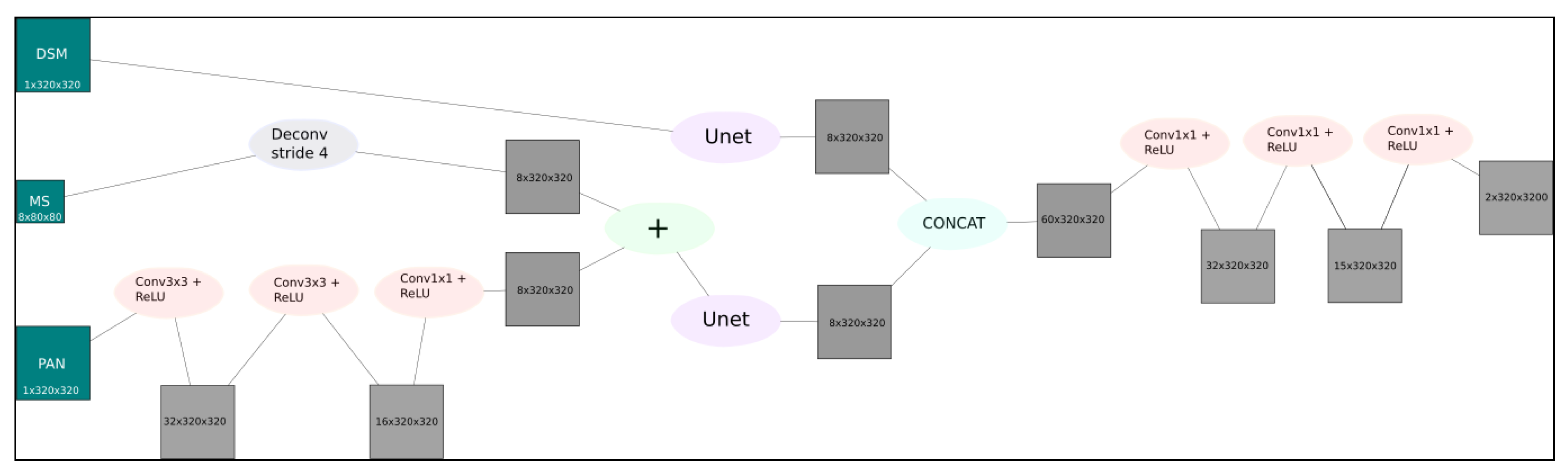
As we want to use multiple data-sources, the emerging question is how to fuse the data-sources efficiently. To reduce the amount of pre-processing, we combine the PAN and the multi-spectral image automatically at an earlier stage similar to Rao et al. [12]. Mainly, we apply transposed convolution to the multi-spectral image to up-sample it by factor four. The PAN is fed to a shallow three-layer FCN to obtain eight feature maps. The output of the transposed convolution and the FCN are added. In this approach, only the sparse residuals between the up-sampled multi-spectral image and the targeted high-resolution feature maps need to be learned by the network. The schematic architecture of the proposed network is depicted in Figure 1.

Figure 1. The complete architecture of the proposed network. The architecture consists of three main stages. In the first stage, the multi-spectral image and the pan image are fused by applying a residual neural network block. The pansharpened output image propagates further to the second stage of the proposed architecture corresponding to the Unet. In a parallel stream, the DSM image also goes through the Unet. In the final stage, two branches are merged by CONCAT layer and further propagate to the top layer of the proposed network.

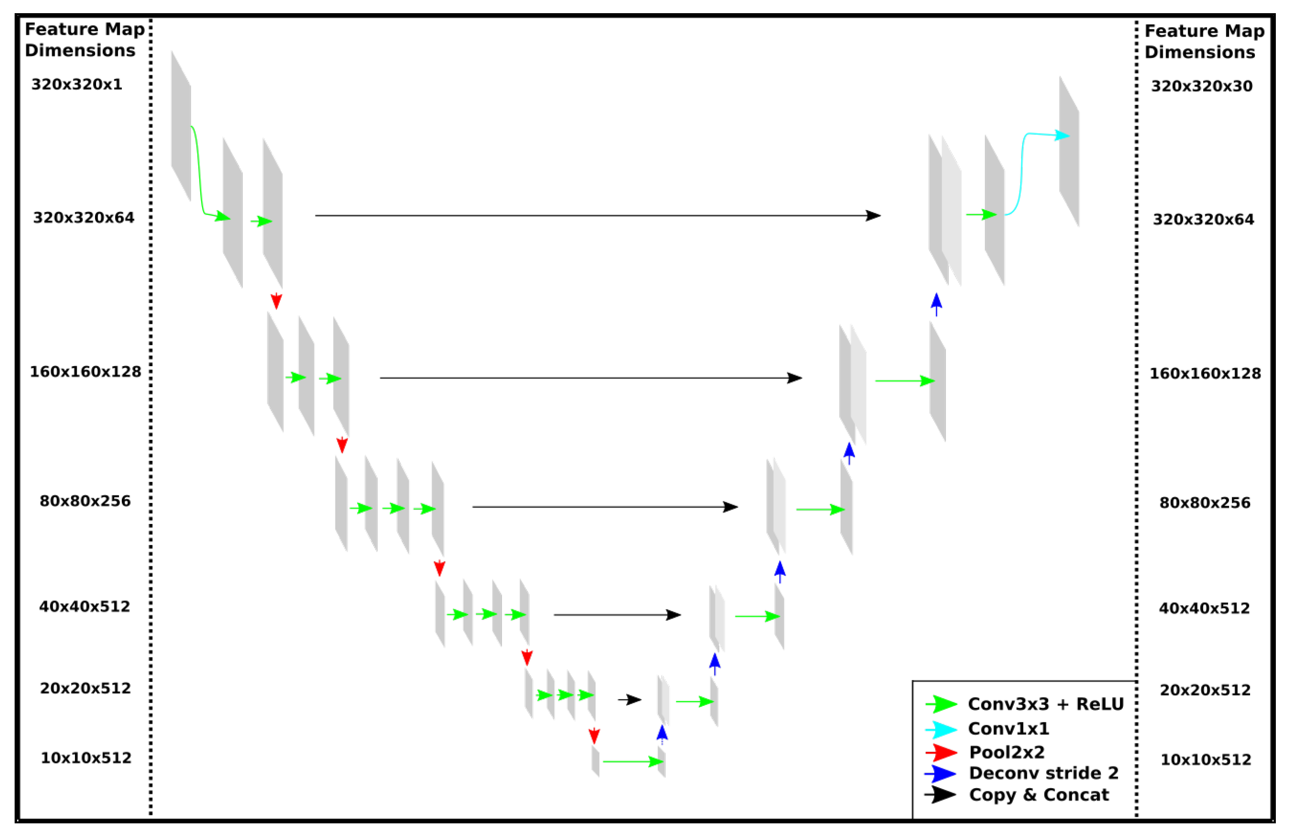
The resulting feature maps and DSM are passed to seperate FCNs. Similar to the Unet introduced by Ronneberger et al. [18], we use a FCN which, for each max-pooling layer, has a transposed convolution layer with the same stride but omit cropping the feature maps to obtain equality of output and input size. As a VGG16-based FCN has shown good results in Bittner et al. [15], Marmanis et al. [13] and Bittner et al. [16], we use its first five layers and then put a sixth layer with 512 $3\times 3$—kernels on top of it to learn the features specific for building footprint extraction. Compared to VGG16, this approach dramatically decreases the number of parameters in the network. Because it keeps the number of parameters low, we only apply one, instead of two, convolutional layers per resolution-level in the decoder, as in Iglovikov and Shvets [17]. The outputs are concatenated and a three-layer deep network is applied. This network automatically learns to recognize the individual contributions of spectral and depth information for extracting the buildings [16]. For a visualization of our adapted Unet architecture see Figure 2.

Figure 2. The proposed adapted Unet architecture.

There are many architecture models that have been trained on huge databases for many iterations. To reduce computational cost and excessive hyperparameter tuning, we use such a model and fine tune it for the task at hand. Specifically, we use an ImageNet pre-trained VGG16, which can be fine tuned for semantic segmentation of remote sensing imagery [13,16]. We use the weights of the first five layers of the VGG16 only for our multi-spectral and PAN data, as the features learned by the pre-trained model are specific for spectral data and are not suitable for the 3D information in the DSM data.

4. Study Area and Experiments

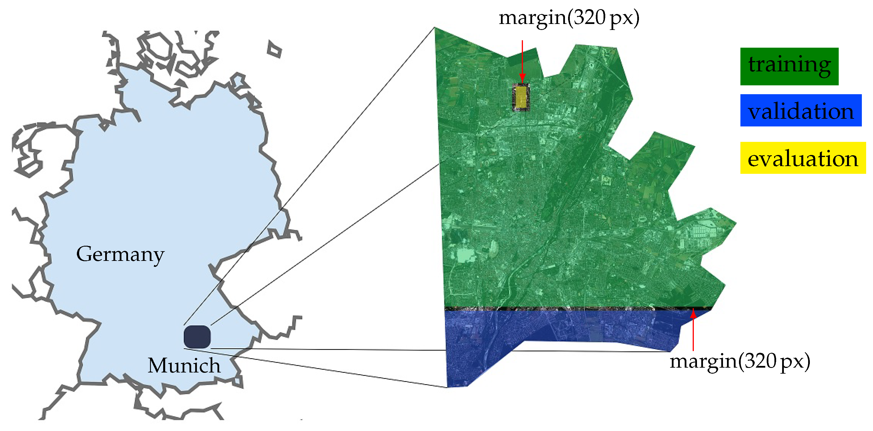
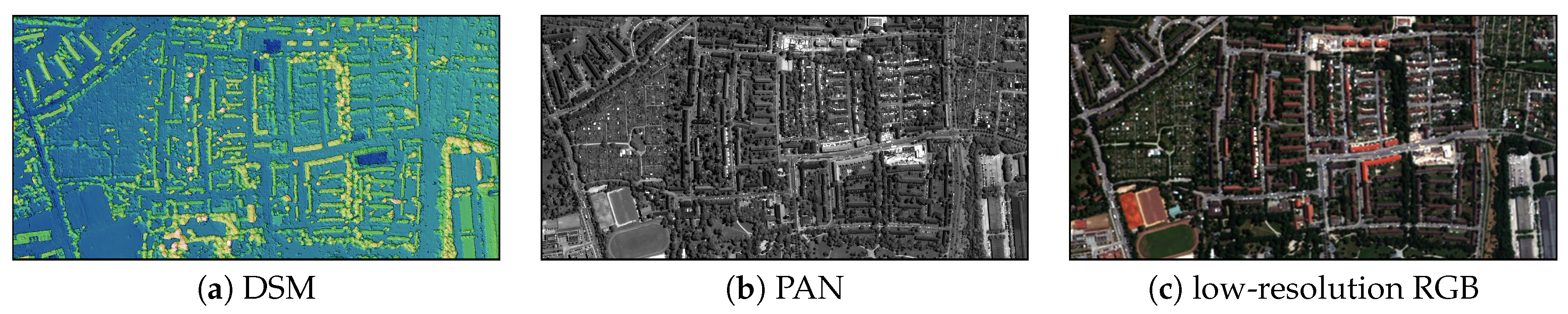
For evaluation of our approach, we use World View-2 imagery of Munich, Germany. An overview of area of interest (AOI) is illustrated in Figure 3. We subdivided the AOI into training, validation and evaluation parts keeping the margin of 320 $\mathrm{px}$ in between to ensure datasets independence. The training data consists of stereo DSM, PAN both $0.5$ $\mathrm{m}$ GSD and 2 $\mathrm{m}$ GSD MS images with 8 channels tiled into a collection of 32.500 patches with a size of $320\times 320$ $\mathrm{px}$ and overlap $160\times 160$ $\mathrm{px}$, where 20% are kept back for validation and the rest for training. 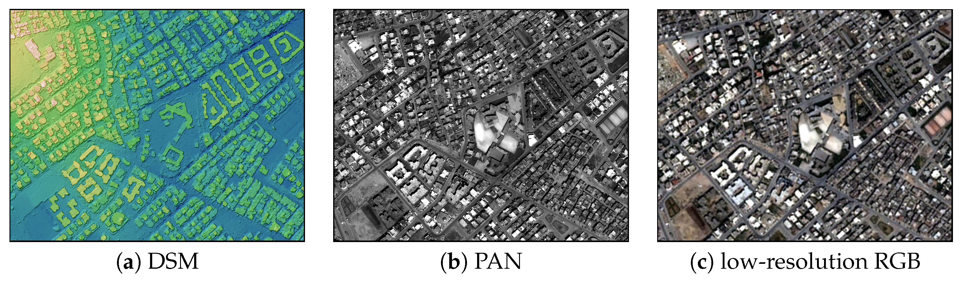A $1280\times 2560$ $\mathrm{px}$ area, which does not overlap with the training data, is used for testing phase (see Figure 4). The satellite images are orthorectified, because we want to obtain building footprints that appear as if they are viewed from nadir. In order to show the generalization capability of our model, we include small parts from World View-2 imagery of urban areas of Tunis, Tunisia (see Figure 5). To compensate for the missing ground truth in this area, we use building footprints from OSM. However, there are only a few areas, which are densely covered by OSM building footprint data. The test regions are acquired by selecting areas where high quality DSM data as well as OSM building footprints are available.

Figure 3. AOI of Munich, Germany. The AOI is further tiled into datasets for training, validation and evaluation. Between the datasets we left a margin of 320 $\mathrm{px}$ to prevent data repetition.

Figure 4. Test area in Munich, Germany. DSM image is color-shaded for better visualization.

Figure 5. The selected area over Tunis, Tunisia used for visual inspection. DSM image is color-shaded for better visualization.

4.1. Image Pre-Processing

We subtract the mean of the whole training data from each patch during training and, while testing, we subtract the mean of the test area. Then, we rescale our data to the range $\left[-1,1\right]$. The raw DSM contains many outliers which enlarge the distribution range dramatically, although the majority of values lay within a much smaller range. Therefore, we follow the strategy applied by Bittner et al. [16] to remove these outliers and use linear spline interpolation to find the values of thresholded points.

4.2. Implementation Details and Training

Based on the code developed by Bittner et al. [16], we implemented our Unet network on top of the Caffe deep learning framework. For training, we use common stochastic gradient descent (SGD) optimization algorithm in small batches for efficiency together with momentum and weight decay. A detailed explanation of this training algorithm is given by Rumelhart et al. [19]. An epoch consists of iteratively feeding mini-batches to the network, computing the gradients and updating the weights, until each patch in the training data has been processed once by the network. Depending on the batch size, the number of iterations in one epoch varies. Due to the memory limit of 12 GB on the used NVIDIA TITAN X (Pascal) GPU, our batch size was limited and was chosen as big as possible for each network.

In Table 1 the training hyperparameters are presented. We obtained their respective value empirically. The learning rate is multiplied by 0.1 every 4 epochs. We give the number of epochs for every trained architecture in Table 2.

Table 1. The hyperparameters used for training. All parameters were obtained empirically during investigation of the training process on the validation dataset.

Initial Learning Rate $\mathit{\lambda }$	Weight Decay $\mathit{\eta }$	Momentum $\mathit{\mu }$	Dropout Rate d
0.001	0.005	0.9	0.5

Table 2. Number of epochs used to train different architectures.

	FCN4s	Unet
Fused	10	-
LateConc	10	-
EarlyConc	8	-
Hybrid	9	8

The patches used for training, validation and test phases overlap by 160 $\mathrm{px}$ within dataset in each dimension and, during inference, the network output is averaged in the overlapping regions. We initialize all weights of convolutional layers which are not filled with pre-trained weigths by uniformly sampled random numbers from the range $\left[-\frac{1}{N},\frac{1}{N}\right]$, where N is the number of neurons for that layer.

4.3. Comparison with Alternative Methods

To compare the network described in Section 3.1.1 to other architectures by means of how well it makes use of the available data and for efficiency, we train and test the Fused-FCN4s proposed by Bittner et al. [16] with pansharpened RGB, PAN and DSM data. In contrast to Bittner et al. [16], we use DSM instead of nDSM. Further, to demonstrate that FCNs can integrate spectral and geometric information without using a pre-processed pansharpened RGB, we introduce LateConc-PAN&RGB&DSM-mrFCN4s network which for the RGB-stream inputs the low-resolution RGB image to a deconvolutional layer and passes its result to the FCN4s. The mrFCN4s specifies multi-resolution FCN4s network. The resulted network fuses two spectral streams (up-sampled RGB and PAN) and depth stream at the top of the architecture, similar to the Fused-FCN4s [16]. Since multi-spectral information is not limited to the RGB channels, we train and test an architecture which input eight spectral bands covering the range from 400 $\mathrm{nm}$ (Coastal) to 1040 $\mathrm{nm}$ (Near-IR2). We name this setup LateConc-PAN&MS&DSM-mrFCN4s network. The multi-spectral bands here are also low-resolution. The rest of this architecture is identical to the Fused-FCN4s [16].

Furthermore, we investigate two different approaches on fusing spectral information at an early stage compared to the LateConc-PAN&MS&DSM-mrFCN4s. Instead of having two separate streams for both spectral images, the FCN4s with early concatenation named EarlyConc-PAN&MS&DSM-mrFCN4s combines right at the beginning the output of the deconvolutional layer for RGB up-sampling with the PAN image. Then it passes the combined output to a single spectral stream FCN4s. To improve a part of the network responsible for pansharpening task, the FCN4s with pansharpening fusion named as Hybrid-PS-FCN4s applies three convolutional layers to the PAN and sums this with the output of the deconvolution layer applied to multi-spectral image instead of concatenation of the PAN with the deconvolution layer applied to multi-spectral image. The schematic representation of presented strategy is depicted in Figure 1. Rao et al. [12] use a slightly different architecture for pansharpening to fuse the spectral images which, instead of a deconvolutional layer, uses up-sampling and has three instead of eight output channels. Finally, we demonstrate that using our adapted Unet instead of FCNs results in straighter building outlines, higher scores on several metrics and reduces the number of parameters in our network significantly. This Unet with integrated pansharpening module for processing multi-resolution images (Hybrid-PS-Unet) performs best among the compared.

5. Results

To evaluate our approach, we test different architectures in three stages. First, we compare the building footprints generated by different models by their appearance. Then, for every model we use several metrics to evaluate them. Last, we test our proposed model on an entirely new area, unseen during training, to examine its generalization capacity.

5.1. Qualitative Evaluation

5.1.1. LateConc-PAN&RGB&DSM-mrFCN4s vs. Fused-FCN4s

As the pre-processing used to obtain a pansharpened RGB image is computationally expensive, we have decided to pass the low-resolution RGB image to a deconvolution layer, before feeding it to the FCN4s. In Figure 6, zoom-ins of the left highlighted area in Figure 7d for both generated building footprints and the ground truth are compared. The LateConc-PAN&RGB&DSM-mrFCN4s produces too small building footprints and the outlines are smoother than those generated by the Fused-FCN4s. However, it still provides a high quality mask and needs less pre-processing.

Figure 6. Detailed comparison of high vs. low resolution RGB information based on FCN4s network. (a) illustrates the results from LateConc-PAN&RGB&DSM-mrFCN4s network, (b) depicts the resulted mask from Fused-FCN4s model and (c) is a ground truth mask.

Figure 7. Generated masks of three different fusion strategies.

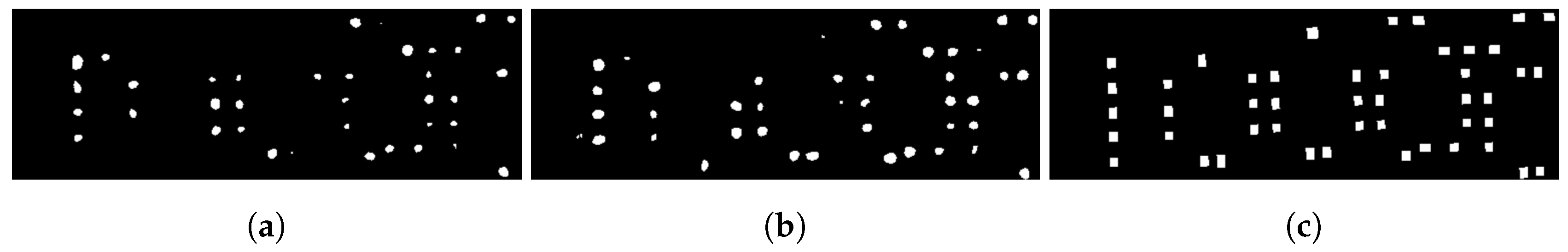
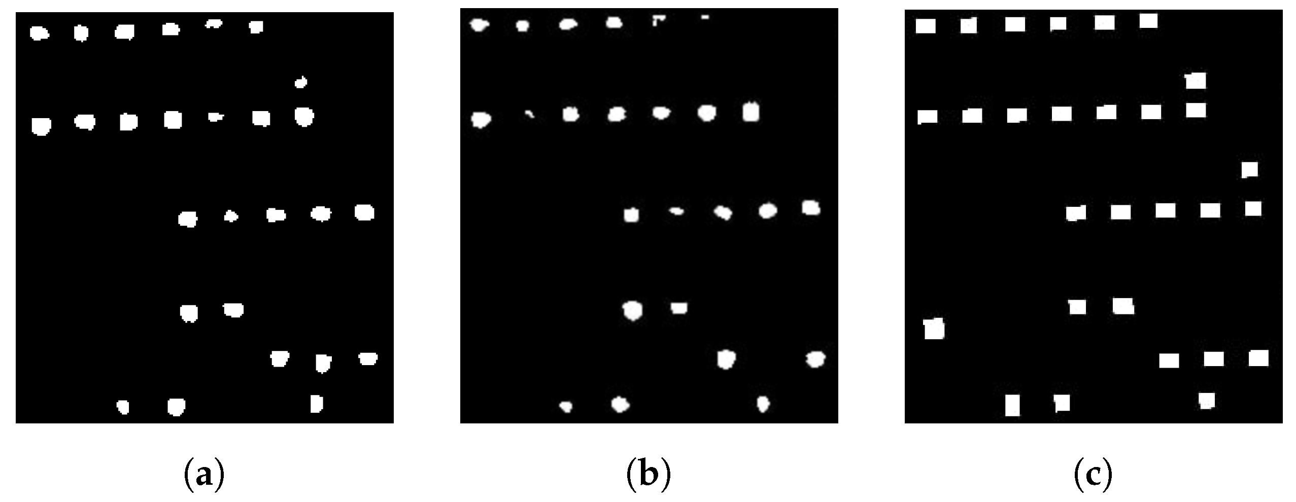
5.1.2. LateConc-PAN&MS&DSM-mrFCN4s vs. LateConc-PAN&RGB&DSM-mrFCN4s

To make the network more powerful, we replace the RGB image with an eight-channel multi-spectral image. We demonstrate the results based on the right zoom-in area in Figure 7d. Investigating the resulted masks in Figure 8a,b, we can notice that the LateConc-PAN&MS&DSM-mrFCN4s detects more small building footprints than the LateConc-PAN&RGB&DSM-mrFCN4s. Comparing both footprints with the ground truth, we can conclude that additional multi-spectral information only slightly increases the number of parameters (see Table 3) of the overall network, but leads to more complete building footprints.

Figure 8. Detailed comparison of multi-spectral vs. RGB information based on FCN4s networks. (a) shows the zoomed area of building mask generated by LateConc-PAN&RGB&DSM-mrFCN4s architecture, (b) illustrates the building mask obtained from LateConc-PAN&MS&DSM-mrFCN4s model and (c) is a ground truth mask.

Table 3. Evaluation results regarding the efficiency. Inference on a NVIDIA GeForce Titan X. The superior values are highlighted in bold.

Architecture	Number Parameters	Time Forward-Pass
Fused-FCN4s	403205772	0.100553875923 s
LateConc-PAN&RGB&DSM-mrFCN4s	403205964	0.100716901302 s
LateConc-PAN&MS&DSM-mrFCN4s	403209164	0.100480812907 s
EarlyConc-PAN&MS&DSM-mrFCN4s	268807592	0.0667015542984 s
Hybrid-PS-FCN4s	268812040	0.0677197296619 s
Hybrid-PS-Unet	56185288	0.0735983946323 s

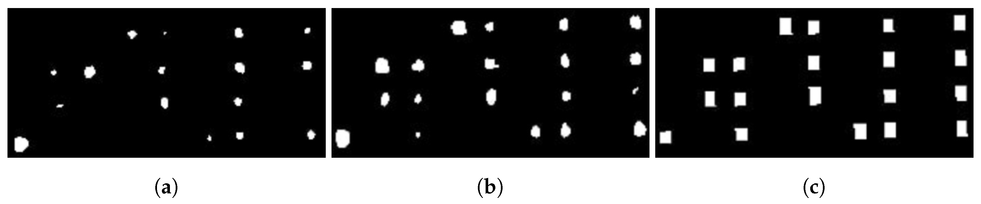
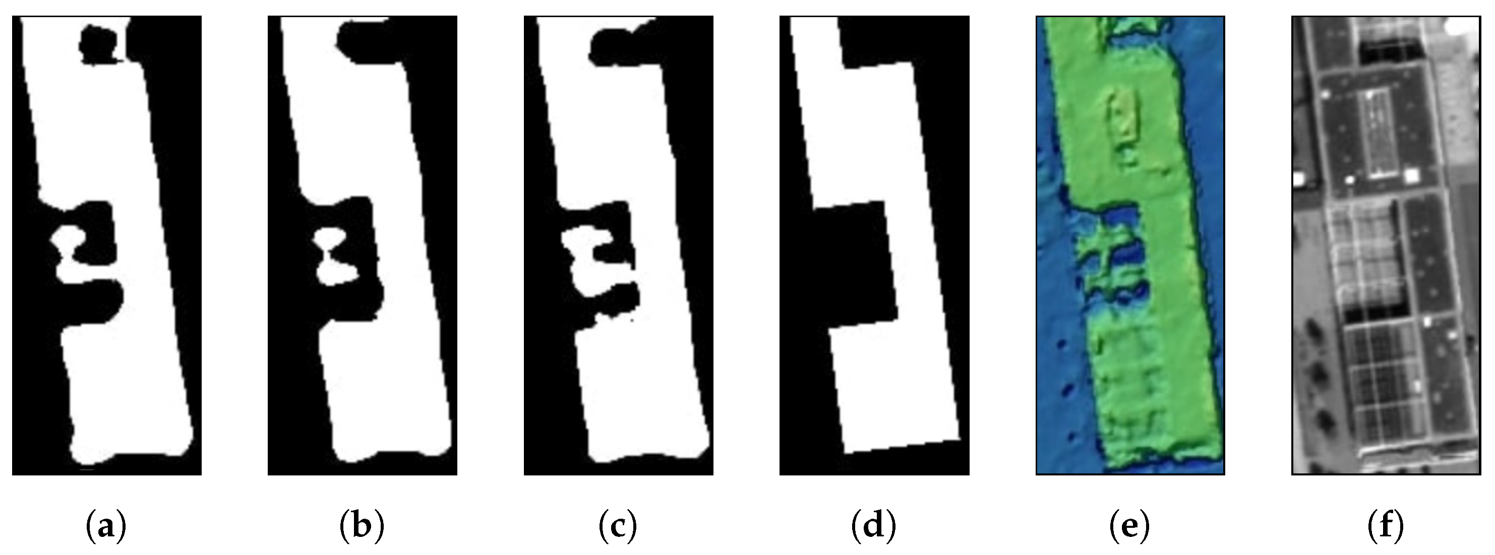
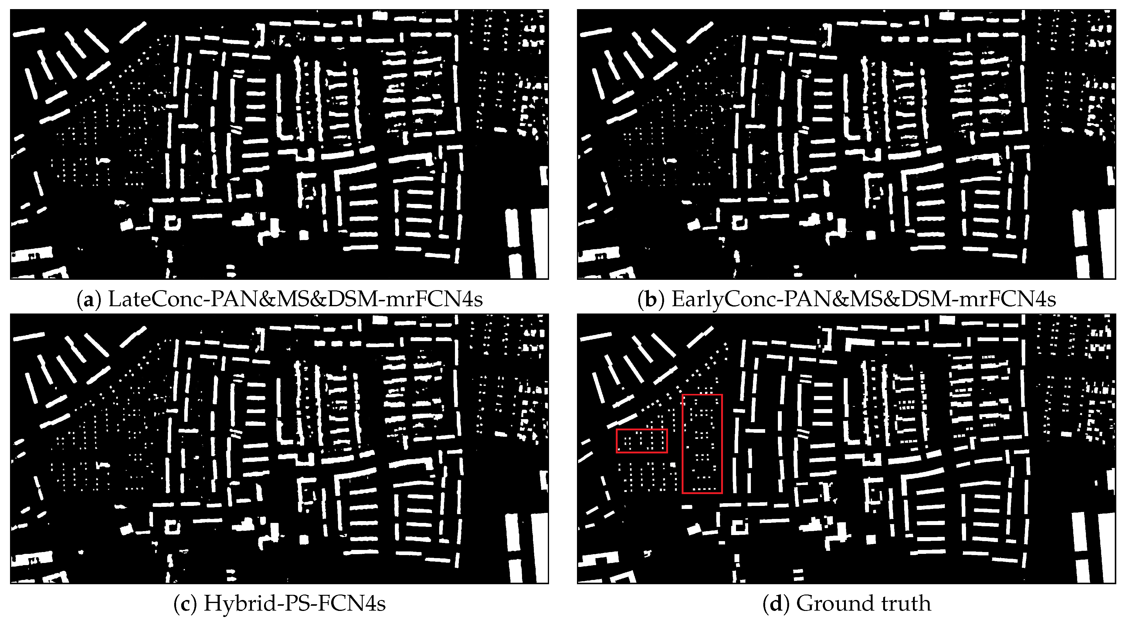
5.1.3. Hybrid-PS-FCN4svs. EarlyConc-PAN&MS&DSM-mrFCN4s vs. LateConc-PAN&MS&DSM-mrFCN4s

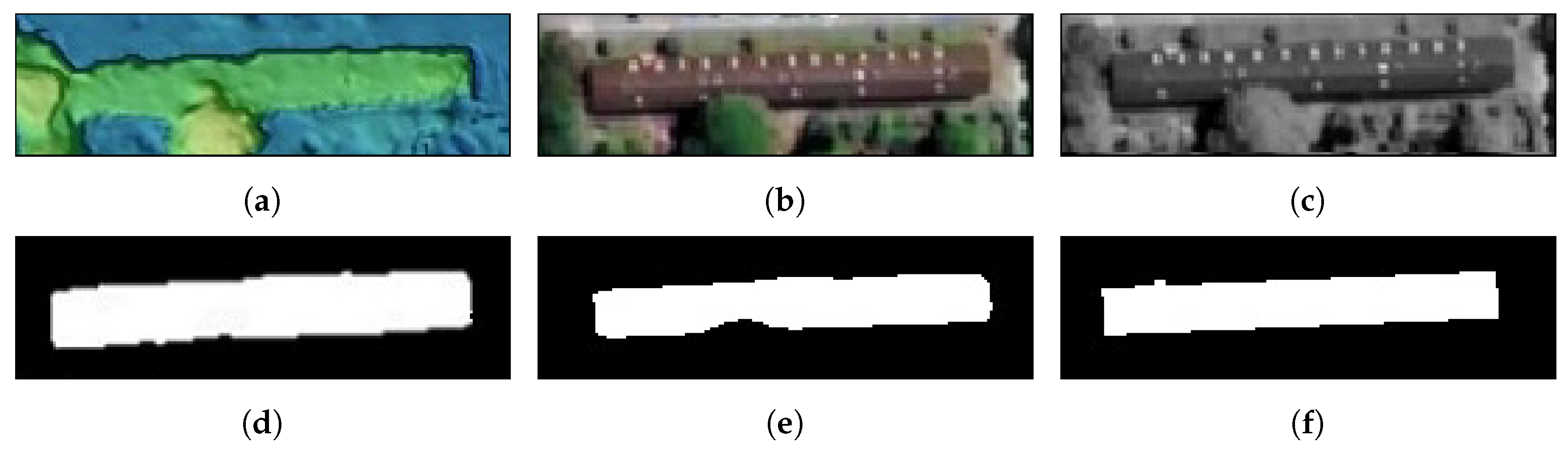
We now compare approaches on fusing images of different resolution. The masks resulted from the experiments are displayed in Figure 7. EarlyConc-PAN&MS&DSM-mrFCN4s model leads to a less accurate mask. This can be seen in the example of selected building illustrated in Figure 9a. Here both the LateConc-PAN&MS&DSM-mrFCN4s and the Hybrid-PS-FCN4sgive more accurate results. In the mask generated by the Hybrid-PS-FCN4swe see additional structures in the middle of the building, which are not present in the ground truth. This building has a glass roof built on a hash-like structure. As we can see in Figure 9, the information is present in our results. It is noteworthy that with a far smaller number of parameters the Hybrid-PS-FCN4sarchitecture performs very similar to the LateConc-PAN&MS&DSM-mrFCN4s.

Figure 9. The detailed comparison between different fusion strategies for binary building mask generation: (a) EarlyConc-PAN&MS&DSM-mrFCN4s, (b) LateConc-PAN&MS&DSM-mrFCN4s, (c) Hybrid-PS-FCN4sand (d) ground truth. (e,f) depict color-shaded DSM and PAN example of selected building, respectively.

5.1.4. Hybrid-PS-Unet vs. Fused-FCN4s

To show the improvements over recent approaches, we tested our proposed Hybrid-PS-Unet against the Fused-FCN4s. Figure 10 shows zoom-ins of the resulting building masks. The boundaries are much sharper in the results of the Unet with pansharpening fusion. In the PAN, we can see that there is a tree that covers some part of a building. As a result, we can conclude that the Hybrid-PS-Unet is able to reconstruct the missing building boundary. Besides, it can produce a rectangular shape without having complete information of the true building outline. The reason might be that the Hybrid-PS-Unet has learned better than the Fused-FCN4s that buildings more often are rectangular.

Figure 10. Detailed comparison of selected building footprints generated by Fused-FCN4s and Hybrid-PS-Unet models. (a) illustrates the building representation on color-shaded DSM, (b,c) show the building on RGB and PAN images, respectively, (d) presents the resulted footprint form Hybrid-PS-Unet model, (e) displays building footprint from Fused-FCN4s network and (f) is a ground truth mask.

Moreover, Figure 11 demonstrates that the Hybrid-PS-Unet recognizes much more of the small buildings. The mask generated by the Fused-FCN4s, on the other hand, misses more of those buildings. The shapes of the produced building footprints have smoother boundaries, compared to footprints from Hybrid-PS-Unet model, and have smaller size compared to the ground truth. In contrast, the building footprints produced by the Hybrid-PS-Unet are very similar to the ground truth.

Figure 11. Detailed comparison of Fused-FCN4s and Hybrid-PS-Unet models. (a) presents the zoom-in area of building mask from Hybrid-PS-Unet model, (b) illustrates the capability of small building footprints generation by Fused-FCN4s and (c) is a ground truth.

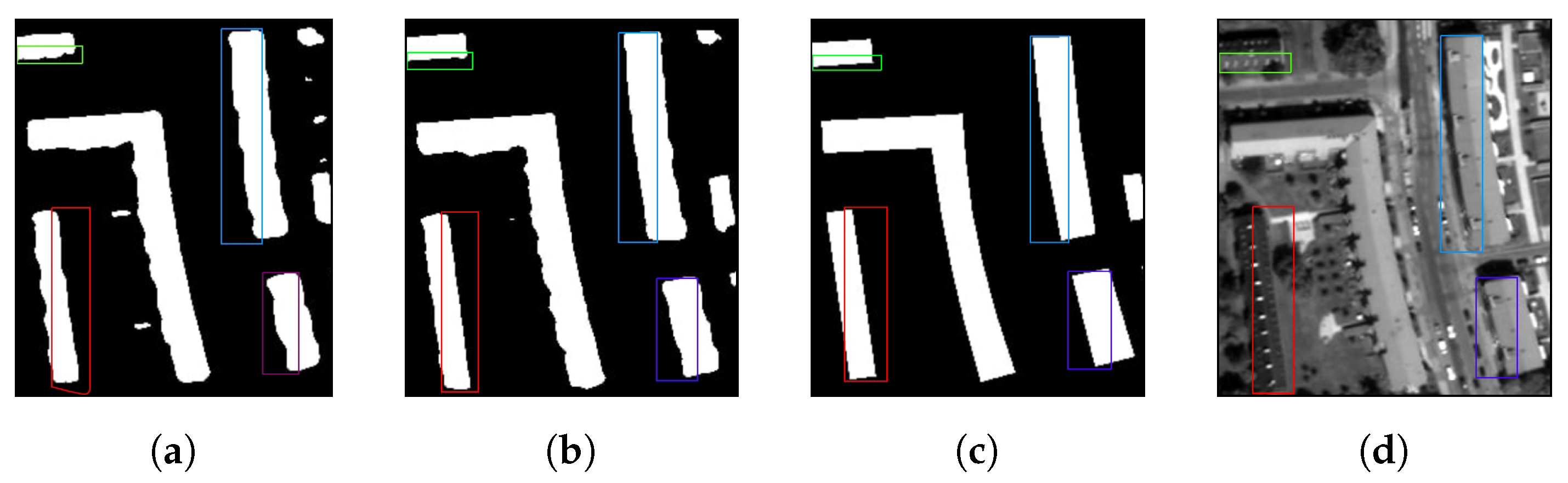
5.1.5. Hybrid-PS-Unet vs. Hybrid-PS-FCN4s

Since it is very important for building footprint masks to have the outlines as straight as possible, we aim to utilize more of the high resolution content of our input images by applying the Unet architecture to our data. Investigating the boundaries of generated building outlines highlighted by colored rectangle in Figure 12, we can notice that the building boundaries produced by Hybrid-PS-Unet modes are less bumpy and more close to the real building representations.

Figure 12. Detailed comparison of results produced by Hybrid-PS-FCN4sand Hybrid-PS-Unet models. (a) demonstrates the results obtained from Hybrid-PS-FCN4smodel, (b) depicts the resulted mask generated by Hybrid-PS-Unet and (c) shows a ground truth. (d) illustrates the real building representation in satellite image.

5.2. Quantitative Evaluation

To quantitatively evaluate the experiments, we use the Overall, Mean Accuracy and Mean IoU as in Long et al. [11],

$$\begin{array}{cc}\hfill \mathrm{Mean}\mathrm{accuracy}& =\frac{1}{n_{cl}}\sum _i\frac{n_{ii}}{t_i},\hfill \end{array}$$

(6)

$$\begin{array}{cc}\hfill \mathrm{Overall}\mathrm{accuracy}& =\frac{1}{n_{cl}}\sum _i\frac{n_{ii}}{t_i+{\sum }_j{n}_{ji}-n_{ii}},\hfill \end{array}$$

(7)

$$\begin{array}{cc}\hfill \mathrm{Mean}\mathrm{IoU}& =\frac{{\sum }_i{n}_{ii}}{{\sum }_i{t}_i},\hfill \end{array}$$

(8)

where $n_{ij}$ is the number of pixels that belongs to class i, but are classified as j, $n_{cl}$ is the number of different classes, and $t_i={\sum }_j{n}_{ij}$ corresponds to the number of pixels that belongs to class i. Additionally, we use the binary classification metrics $precision$ (Prec.), $recall$ (Rec.), $IoU$ and $F_1$-measure

$$\begin{array}{c}\mathrm{Precision}=\frac{TP}{FP+TP},\end{array}$$

(9)

$$\begin{array}{c}\mathrm{Recall}=\frac{TP}{FN+TP},\end{array}$$

(10)

$$\begin{array}{c}\mathrm{IoU}=\frac{TP}{TP+FP+FN},\end{array}$$

(11)

$$\begin{array}{c}{F}_1=\frac{2TP}{2TP+FP+FN},\end{array}$$

(12)

where $TP$, $FP$, $FN$ denote the total number of true positive, true negative, false positive and false negative, respectively. The $precision$ indicates how well a binary classifier avoids to classify a non-pixel as a building pixel, whereas the $recall$ indicates how well a classifier avoids missing building pixels. The $F_1$-measure is the special case of the $F_{\beta }$-measure, where $\beta =1$ and equivalent to the harmonic mean

$$F_1=\frac{2\times precision\times recall}{precision+recall}$$

(13)

of $precision$ and $recall$. In our data, the number of building pixels is much smaller than non-building pixels. Thus, the $IoU$ is the hardest of those three metrics to obtain a high score from, because the number of building pixels is much smaller than non-building pixels and the $IoU$ can only be high if TP is high.

We list the results of evaluated metrics on the Fused-FCN4s architecture developed by Bittner et al. [16], the LateConc-PAN&RGB&DSM-mrFCN4s, LateConc-PAN&MS&DSM-mrFCN4s, EarlyConc-PAN&MS&DSM-mrFCN4s, Hybrid-PS-FCN4s as well as the Hybrid-PS-Unet architectures in Table 4. The number of parameters as well as the inference speed are given in Table 3. From the statistics in Table 4 we recognize that the architectures which use a pansharpened RGB, or implicitly produce a pseudo pansharpened multi-spectral image are significantly worse on $IoU$ than on the other metrics. Furthermore, we note that the Hybrid-PS-Unet performs slightly better than the FCN4s-based architectures. Despite the lower overall number of layers and the lower number of kernels in the bottleneck, the Hybrid-PS-Unet architecture performs better than all other architectures on all metrics. The obtained results are very accurate, which points out that (a) no post-processing is necessary and (b) DSM is a suitable substitute for nDSM when given to the Hybrid-PS-Unet. There are three experiments, where the $precision$ is much higher than the $recall$. In the corresponding building footprints, many building pixels are missed, whereas fewer pixels are incorrectly classified as building pixels. Remarkably, the Hybrid-PS-Unet is the only architecture which produced a higher $recall$ than $precision$. This matches with the results of the visual inspection, where we found that the Hybrid-PS-Unet recognized building pixels covered by trees better than the other architectures.

Table 4. Quantitative results of the examined architectures, given in percent. The superior values are highlighted in bold.

	RGB		MS			Metrics
	Fused	Late Conc	Late Conc	Early Conc	Hybrid	Mean Acc.	Acc.	IoU	Mean IoU	Prec.	Rec.	${\mathit{F}}_{\mathbf{1}}$
FCN4s	x					93.7	97.2	80.3	88.6	89.1	89.1	89.1
mrFCN4s		x				91.4	96.8	77.2	86.8	90.3	84.2	87.1
mrFCN4s			x			92.3	97.0	78.6	87.6	90.2	86.0	88.0
mrFCN4s				x		92.1	96.8	77.5	87.0	88.9	85.8	87.3
mrFCN4s					x	93.5	97.2	80.1	88.5	89.4	88.5	88.9
UNet					x	94.4	97.4	81.7	89.4	89.5	90.3	89.9

5.3. Model Generalization Capability

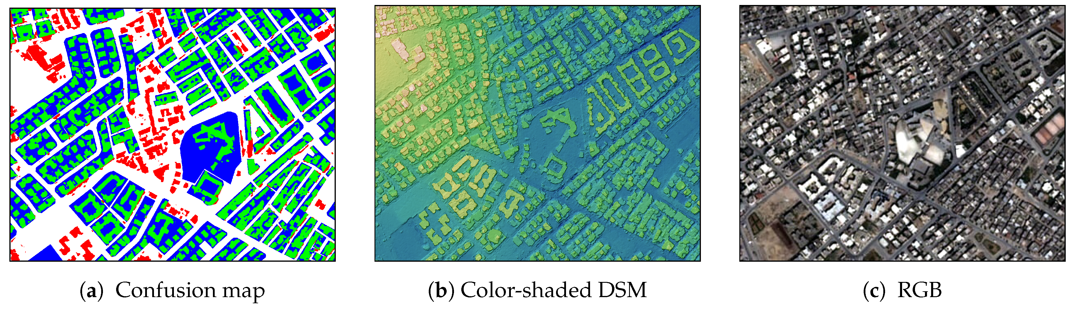
To study the models capacity to extract the key features distinguishing buildings from non-buildings, we employ it on data from Tunis, Tunisia. Other than in Munich data, the Tunis images contain more complex rooftop textures. Further challenges on this dataset are the very high grade of detail of the building outlines and the high variations in building density. The Tunis test data was directly passed to the system that was only trained on Munich data. In Figure 13 we can see that the resulting building footprints are much more detailed than the groundtruth obtained from OSM. Many details and even some complete buildings, which we can determine in Figure 13, are missing in the OSM data but are present in the predicted mask. From visual inspection we can see that the model generalizes well on the Tunis images. It captures fine details and highly complex building structures and operates independently from building density.

Figure 13. Comparison of OSM data and a footprint mask generated by the proposed Hybrid-PS-Unet model with pansharpening fusion. In (a), at locations with green pixels, both OSM and our model predict building. At white pixels, our architecture and the OSM data predict non-building. At locations with red pixels, our architecture predicts building and the OSM data predicts non-building. At pixels with blue colours, the OSM data predicts building and our model predicts non-building.

6. Discussion

First, the experiments carried out on the fusion strategy showed that the EarlyConc-PAN&MS&DSM-mrFCN4s does not perform as good as LateConc-PAN&MS&DSM-mrFCN4s and Hybrid-PS-FCN4s. The approach implies concatenation of one PAN channel with the eight outputs of the transposed convolution of the multi-spectral image. Therefore, the amount of information forwarded to the next layer is strongly imbalanced, with only a small proportion of the PANs high spatial resolution. Despite late fusion performs better than early concatenating, it does not take into account that PAN and multi-spectral images share many common features. For example, a shape typical for a building might be recognized by the network by its geometrical appearance in both image signals. The pansharpening fusion avoids this redundancy and balances the proportions of information proceeded to the next layer by both images.

Furthermore, the applied pre-processing involved the normalization of the images, which had a huge influence on the results. During development, tests with not equally scaled images as those in the training set showed poor results. Artifacts were introduced by the network, which are hard to interpret from the given images. This shows that the network learned scale specific. Also, it is very important to apply the same re-scaling method to all data sources. Even though the network could learn to balance differently scaled data, this takes an extra effort, hampering the training process. Also the generation process of stereo DSM images produces outliers which influence the histogram of the values in the DSM. Ignoring the outliers leads to misbehaviour during training and testing, as it affects the mean value. Subtracting a mean which is excessively high due to outliers, pushes the true values far away from the mean. In effect, re-scaling narrows the range of the true values, whereas we want them to share the whole range of possible values. Thus, it is important to handle the outliers properly.

The performance of a model should not only be evaluated based on metrics, e.g., IoU, but also based on the number of free parameters, which are adapted by SGD steps. The larger this number, the longer the training of the network takes. This is due to the fact that a smaller model can use larger mini-batches, which makes the gradient estimations more accurate and increases the exploitation of the potential for parallelisation on a GPU. Also, a lower number of parameters corresponds to faster forward passes in training and testing.

When comparing our results to those in other papers, it is important to be aware of the respective training dataset. In general, larger training datasets can cover a greater amount of buildings and variety of building appearances, allowing the network to produce scores with higher certainty and generalize better. Even if the amount of training data is high, bad quality of the ground truth can influence the results and causes uncertainty on incorrectly labelled features, or can make testing difficult, as seen in Section 5.3.

7. Conclusions

We adapt the Unet architecture to very high resolution (VHR) remote sensing imagery for the task of building footprint extraction and show that it can provide building masks of high quality. Furthermore, we present a method to fuse depth and spectral information based on fully convolutional network (FCN)s. The developed architecture provides an end-to-end framework for semantic segmentation, which performs well on the task of building footprint extraction from World View2 images. The trained system was tested on unseen urban areas in Munich, Germany and Tunis, Tunisia. It produces masks with sharper edges and has less parameters than the reference architecture. Moreover, it works with digital surface models (DSMs) and low-resolution multi-spectral images. Using eight multi-spectral bands instead of three increased the quality of the extracted masks. The performance of the proposed architecture does not depend on simple or reoccurring shapes, but segments complex and very small building structures accurately. Some of the remaining noise and inaccuracies in the generated building masks is often due to the trees covering whole buildings, ongoing construction work or complex building structures. Although the improvement in quality of our method is small, it still excels the performance of the reference architecture, while having far less parameters and higher inference speed. Therefore, we believe that the presented method has a great potential to efficiently exploit mixed datasets of remote sensing imagery for building footprint extraction.

References

- Huertas, A.; Nevatia, R. Detecting Buildings in Aerial Images. Comput. Vis. Graph. Image Process. 1988, 41, 131–152. [Google Scholar] [CrossRef]
- Guercke, R.; Sester, M. Building Footprint Simplification Based on Hough Transform and Least Squares Adjustment. In Proceedings of the 14th Workshop of the ICA Commission on Generalisation and Multiple Representation, Paris, France, 30 June–1 July 2011. [Google Scholar]
- Brédif, M.; Tournaire, O.; Vallet, B.; Champion, N. Extracting polygonal building footprints from digital surfce models: A fully-automatic global optimization framework. ISPRS J. Photogramm. Remote Sens. 2013, 77, 57–65. [Google Scholar] [CrossRef]
- Ekhtari, N.; Sahebi, M.R.; Zoej, M.J.V.; Mohammadzadeh, A. Automatic building extraction from LIDAR digital elevation models and WorldView imagery. J. Appl. Remote Sens. 2009, 3, 033571. [Google Scholar] [CrossRef]
- Rottensteiner, F.; Trinder, J.; Clode, S.; Kubik, K.; Lovell, B. Building Detection by Dempster-Shafer Fusion of LIDAR Data and Multispectral Aerial Imagery. In Proceedings of the 17th International Conference on Pattern Recognition, Cambridge, UK, 26 August 2004. [Google Scholar]
- Turlapaty, A.; Du, Q.; Gokaraju, B.; Younan, N.H. A Hybrid Approach fo Building Extraction from Spaceborne Multi-Angular Optical Imagery. IEEE J. Sel. Top. Appl. Earth Obs. Remote Sens. 2012, 5, 89–100. [Google Scholar] [CrossRef]
- LeCun, Y.; Bottou, L.; Bengio, Y.; Haffner, P. Gradient-Based Learning Applied to Document Recognition. Proc. IEEE 1998, 86, 2278–2324. [Google Scholar] [CrossRef]
- Krizhevsky, A.; Sutskever, I.; Hinton, G.E. Imagenet Classification with Deep Convolutional Neural Networks. In Proceedings of the Advances in Neural Information Processing Systems 25: 26th Annual Conference on Neural Information Processing Systems 2012, Lake Tahoe, NV, USA, 3–6 December 2012. [Google Scholar]
- Simonyan, K.; Zisserman, A. Very Deep Convolutional Networks for Large-Scale Image Recognition. arXiv 2014, arXiv:1409.1556. [Google Scholar]
- He, K.; Zhang, X.; Ren, S.; Sun, J. Deep Residual Learning for Image Recognition. arXiv 2015, arXiv:1512.03385. [Google Scholar]
- Long, J.; Shelhamer, E.; Darell, T. Fully convolutional networks for semantic segmentation. In Proceedings of the IEEE Conference on Computer Vision and Pattern Recognition, Boston, MA, USA, 7–12 June 2015; pp. 3431–3440. [Google Scholar]
- Rao, Y.; He, L.; Zhu, J. A residual convolutional neural network for pan-shaprening. In Proceedings of the 2017 International Workshop on Remote Sensing with Intelligent Processing (RSIP), Shanghai, China, 18–21 May 2017. [Google Scholar]
- Marmanis, D.; Wegner, J.D.; Galliani, S.; Schindler, K.; Datcu, M.; Stilla, U. Semantic segmentation of aerial images with an enselmble of cnns. ISPRS Ann. Photogramm. Remote Sens. Spat. Inf. Sci. 2016, 3, 473–480. [Google Scholar] [CrossRef]
- Maggiori, E.; Tarabalka, Y.; Charpiat, G.; Alliez, P. Convolutional neural networks for large-scale remote sensing image classification. IEEE Trans. Geosci. Remote Sens. 2017, 55, 645–657. [Google Scholar] [CrossRef]
- Bittner, K.; Cui, S.; Reinartz, P. Building extraction from remote sensing data using fully convolutional networks. Int. Arch. Photogramme. Remote Sens. Spat. Inf. Sci. 2017, XLII-1/W1, 481–486. [Google Scholar] [CrossRef]
- Bittner, K.; Adam, F.; Cui, S.; Körner, M.; Reinartz, P. Building footprint extraction from VHR remote sensing images combined with normalized DSMs using fused fully convolutional networks. IEEE J. Sel. Top. Appl. Earth Obs. Remote Sens. 2018, 11, 2615–2629. [Google Scholar] [CrossRef]
- Iglovikov, V.; Shvets, A. TernausNet: U-Net with VGG11 Encoder Pre-Trained on ImageNet for Image Segmentation. arXiv 2018, arXiv:1801.05746. [Google Scholar]
- Ronneberger, O.; Fischer, P.; Brox, T. U-Net: Convolutional Networks for Biomedical Image Segmentation. In Proceedings of the Medical Image Computing and Computer-Assisted Intervention (MICCAI), Munich, Germany, 5–9 October 2015; LNCS; Springer: Cham, Switzerland, 2015; Volume 9351, pp. 234–241. [Google Scholar]
- Rumelhart, D.E.; Hinton, G.E.; Williams, R.J. Learning representations by back-propagating errors. Nature 1986, 323, 533. [Google Scholar] [CrossRef]
Figure 1.
The complete architecture of the proposed network. The architecture consists of three main stages. In the first stage, the multi-spectral image and the pan image are fused by applying a residual neural network block. The pansharpened output image propagates further to the second stage of the proposed architecture corresponding to the Unet. In a parallel stream, the DSM image also goes through the Unet. In the final stage, two branches are merged by CONCAT layer and further propagate to the top layer of the proposed network.
Figure 2.
The proposed adapted Unet architecture.
Figure 3.
AOI of Munich, Germany. The AOI is further tiled into datasets for training, validation and evaluation. Between the datasets we left a margin of 320 to prevent data repetition.
Figure 4.
Test area in Munich, Germany. DSM image is color-shaded for better visualization.
Figure 5.
The selected area over Tunis, Tunisia used for visual inspection. DSM image is color-shaded for better visualization.
Figure 6.
Detailed comparison of high vs. low resolution RGB information based on FCN4s network. (a) illustrates the results from LateConc-PAN&RGB&DSM-mrFCN4s network, (b) depicts the resulted mask from Fused-FCN4s model and (c) is a ground truth mask.
Figure 7.
Generated masks of three different fusion strategies.
Figure 8.
Detailed comparison of multi-spectral vs. RGB information based on FCN4s networks. (a) shows the zoomed area of building mask generated by LateConc-PAN&RGB&DSM-mrFCN4s architecture, (b) illustrates the building mask obtained from LateConc-PAN&MS&DSM-mrFCN4s model and (c) is a ground truth mask.
Figure 9.
The detailed comparison between different fusion strategies for binary building mask generation: (a) EarlyConc-PAN&MS&DSM-mrFCN4s, (b) LateConc-PAN&MS&DSM-mrFCN4s, (c) Hybrid-PS-FCN4sand (d) ground truth. (e,f) depict color-shaded DSM and PAN example of selected building, respectively.
Figure 10.
Detailed comparison of selected building footprints generated by Fused-FCN4s and Hybrid-PS-Unet models. (a) illustrates the building representation on color-shaded DSM, (b,c) show the building on RGB and PAN images, respectively, (d) presents the resulted footprint form Hybrid-PS-Unet model, (e) displays building footprint from Fused-FCN4s network and (f) is a ground truth mask.
Figure 11.
Detailed comparison of Fused-FCN4s and Hybrid-PS-Unet models. (a) presents the zoom-in area of building mask from Hybrid-PS-Unet model, (b) illustrates the capability of small building footprints generation by Fused-FCN4s and (c) is a ground truth.
Figure 12.
Detailed comparison of results produced by Hybrid-PS-FCN4sand Hybrid-PS-Unet models. (a) demonstrates the results obtained from Hybrid-PS-FCN4smodel, (b) depicts the resulted mask generated by Hybrid-PS-Unet and (c) shows a ground truth. (d) illustrates the real building representation in satellite image.
Figure 13.
Comparison of OSM data and a footprint mask generated by the proposed Hybrid-PS-Unet model with pansharpening fusion. In (a), at locations with green pixels, both OSM and our model predict building. At white pixels, our architecture and the OSM data predict non-building. At locations with red pixels, our architecture predicts building and the OSM data predicts non-building. At pixels with blue colours, the OSM data predicts building and our model predicts non-building.