Article

Detecting Large-Scale Urban Land Cover Changes from Very High Resolution Remote Sensing Images Using CNN-Based Classification

1
School of Remote Sensing and Information Engineering, Wuhan University, 129 Luoyu Road, Wuhan 430079, China
2
Department of Physical Geography, Faculty of Geoscience, Utrecht University, Princetonlaan 8, 3584 CB Utrecht, The Netherlands
*
Author to whom correspondence should be addressed.
Co-first author.
ISPRS Int. J. Geo-Inf. 2019, 8(4), 189; https://doi.org/10.3390/ijgi8040189
Submission received: 9 March 2019 / Revised: 5 April 2019 / Accepted: 9 April 2019 / Published: 11 April 2019

Abstract

:
The study investigates land use/cover classification and change detection of urban areas from very high resolution (VHR) remote sensing images using deep learning-based methods. Firstly, we introduce a fully Atrous convolutional neural network (FACNN) to learn the land cover classification. In the FACNN an encoder, consisting of full Atrous convolution layers, is proposed for extracting scale robust features from VHR images. Then, a pixel-based change map is produced based on the classification map of current images and an outdated land cover geographical information system (GIS) map. Both polygon-based and object-based change detection accuracy is investigated, where a polygon is the unit of the GIS map and an object consists of those adjacent changed pixels on the pixel-based change map. The test data covers a rapidly developing city of Wuhan (8000 km2), China, consisting of 0.5 m ground resolution aerial images acquired in 2014, and 1 m ground resolution Beijing-2 satellite images in 2017, and their land cover GIS maps. Testing results showed that our FACNN greatly exceeded several recent convolutional neural networks in land cover classification. Second, the object-based change detection could achieve much better results than a pixel-based method, and provide accurate change maps to facilitate manual urban land cover updating.

1. Introduction

Quantifying changes in urban land cover has important implications in surveying, mapping, transportation, city planning, economic forecasting, etc., as cities are the major places for human activities. When detecting new land cover types are the objective, urban change detection is specified to a classification-based change detection that attempts to answer the question of “from-to”. Classification-based change detection firstly produces classification maps and then finds changes between labeled pixels or objects of classification maps of different time stamps. If an outdated land cover GIS maps from which changes are to be detected is available, the change map could be produced by comparing the GIS maps and the classification map of recent remote sensing images [1,2]. Our study focuses on a similar task as [2], where a change map is produced for guiding GIS map updating, but introduces deep learning-based methods to automatically learn the optimal features from very-high-resolution (VHR) remote sensing images for classification instead of designing empirical features. In addition, our study site covers an 8000 km2 rapidly developing city, the complexity and dynamics of which constitute challenges for different algorithms and could, therefore, better distinguish and evaluate the algorithms.
A “from-to” change detection task could be realized by pixel-based or object-based approaches. A comprehensive review of change detection [3] stated that object-based approaches [2,3,4] have been taking over pixel-based methods [5,6], as the latter does not fully consider spatial context. An object-based method could be roughly grouped into two categories: with or without using land cover GIS data [7]. Without GIS data, the object could be an arbitrary group of pixels sharing similar properties [2]. One example is the work of [8], where over-segmented polygons are treated as objects. However, this way must introduce pre-segmentation uncertainty and is only used when a GIS map is unavailable. When GIS data is introduced, the object is usually defined by the polygons in a GIS map, and each of them represents a class instance of land use or land cover. The advantage of introducing GIS data is that the data-dependent parameter settings of pixel grouping and the setting of a threshold for change/no change could be avoided. In rare cases when the outdated GIS map and the recent remote sensing images have considerable ground resolution or level of detail (LOD) differences, the conversion error between them will be nonnegligible [9].
In a “from-to” change detection, image classification plays a central role to provide semantic segmentation maps through extracting empirical features from original images. The features, such as pixel value [10], covariance, vegetation index [11,12], texture [13], shadowing effects [14], could vary considerably with different data and therefore affect empirical settings of parameter thresholds. The deep learning-based methods could extract optimal feature representations automatically through multiple neuron layers abstraction, which effectively avoid handcrafted feature design and parameter setting [15]. Deep learning-based methods also blur the boundary between pixel-based and object-based approaches, because they predict a pixel-wise classification map with highly semantic abstraction of spatial context from original remote sensing data. Fully convolutional network (FCN) is a structure of convolutional neural network (CNN) and is one of the most powerful algorithms for semantic segmentation of optical images including those from remote sensors [16]. FCN directly and efficiently learns an equal-sized segmentation map from an input image, instead of learning pixel-by-pixel.
However, the current CNN-based segmentation methods, such as FCN [17], U-Net [18], and DeepLab [19], are commonly developed from the computer vision benchmarks consisting of close range images. One of the biggest problems when applying an FCN to large-size remote sensing images is the scale effect. One class of land cover objects in VHR images commonly varies in a wide range of scales, e.g., a small pool and a large lake (labeled as water), or a separate building and dense residential quarters (labeled as a building). To learn distinctive representations of certain objects from VHR remote sensing images, an FCN-based classification algorithm is required to possess a large receptive field to cover large objects for scale invariance. Feature pyramids have been introduced to U-Net and FPN [20] to partially address the scale problem. Based on these structures, the features at each scale were aggregated to obtain scale robust representations for building segmentation from VHR aerial images [21,22].
A very recent special convolution operator, named Dilated/Atrous convolution [23], has been introduced to FCN to expand the receptive field in a single convolution, and has been introduced to several mainstream segmentation algorithms in computer vision [19,24,25]. The Dilated/Atrous convolution has important implications in classifying large objects from large-size remote sensing data [26], but has not been thoroughly studied.
This study aims at updating a large-scale urban land cover GIS map with recent VHR images using classification-based change detection technology. Firstly, land cover classification map of current VHR images is produced by a proposed CNN structure with full Atrous convolution. Then, a difference map is generated by comparing the classification map with the outdated GIS map, and the later has been pre-converted to a raster land cover map. The difference map is a pixel-wise “from-to” change map. As many articles [27,28] have showed, an object-based change map could obtain a better accuracy and is easy to interpret by a human user than a pixel based one, we translate a pixel-based change map to an object-based change map by two definitions of an “object”. The first definition treats each polygon of the GIS map as an instance of objects, the change map is called a polygon-based change map. The second definition treats a patch consisting of connected change pixels in the difference map as a changed object, within which if the truly changed pixels exceed a given threshold compared to the ground truth, it is regarded as a correctly detected change.
In summary, by using existing GIS maps, our method could avoid the subjective and data-dependent setting of thresholds, which has been a critical problem in most change detection approaches. This is also the main difference between our method and very recent CNN-based classification and change detection methods [8,16,26]. In contrast to other GIS data supported change detection studies [2], we aim at developing advanced deep learning-based methods, specifically, a series of Atrous convolution layers to learn scale robust representations with a large cover of receptive field, to improve land cover classification performance from VHR images. To our knowledge, this study is the first one evaluating new deep learning-based approach on change detection of a city that is big and rapidly growing at multiple, namely, pixel, polygon and object levels.

2. Methodology

2.1. Network for Land Cover Segmentation

We propose a novel and scale robust FCN featuring a very large receptive field. The network backbone is based on a feature pyramid network (FPN) [20] and a ladder-structured U-Net [18], which is capable of learning multi-scale representations. In the encoder, we introduce multi-rate Atrous convolutions in each scale to greatly expand the receptive field of a single convolution, with which objects of different sizes are covered and especially the features of a large object, instead part of it, could be learned.
Figure 1a shows the network structure of our full Atrous convolutional neural network (FACNN). In the encoder, the input features of each scale are convoluted by the Atrous convolution with a rate of 1, 2, and 3 sequentially. As is shown in Figure 1b, the blue and red pixels constitute an Atrous convolution kernel, with the red pixel center of the kernel. The white pixels are skipped when the rate is >1. An Atrous convolution with rate = 3 therefore has a receptive field of 7 × 7 instead of 3 × 3. The FACNN is inspired by [25], which demonstrated that using a different rate of convolution in the same scale could help to eliminate the grid effects that may exist in the same rate Atrous convolution. In our case, this structure is expected to be robust against the multi-scale effects from different sizes of objects in VHR remote sensing images. The rectified linear unit (ReLU) [29] function is chosen as the non-linear activation after each convolution, followed by a batch normalization (BN) [30]. At the fourth scale, features are operated by an Atrous spatial pyramid pooling (ASPP) [19], which is the concatenation of several Atrous convolutions with different rates. The ASPP extensively expands the receptive field of the highest semantic layer. Particularly, with a maximum rate of 18, a pixel could interact with the most part of a 512 × 512 input image.
The structure of decoder (the right side of Figure 1a) is similar to [18]. The first convolutional layer of a low scale is firstly concatenated with the corresponding layer from the encoder and the last convolutional layer of the current scale is up-sampled to the next scale until reaching to the original scale. Softmax is used to translate the last feature maps to a classification map with the same size and resolution of the input image.
The network structure is implemented with the Keras platform (version 2.20) using a TensorFlow backend (version 1.4.0) on Windows 10 system. A Nvidia 1080 TI 11 G GPU is used for training. In the training process, the learning rate is set to 0.0001 and the batch size is set to 4, the Adam (adaptive moment estimation) algorithm is used as the optimizer.

2.2. Change Detection

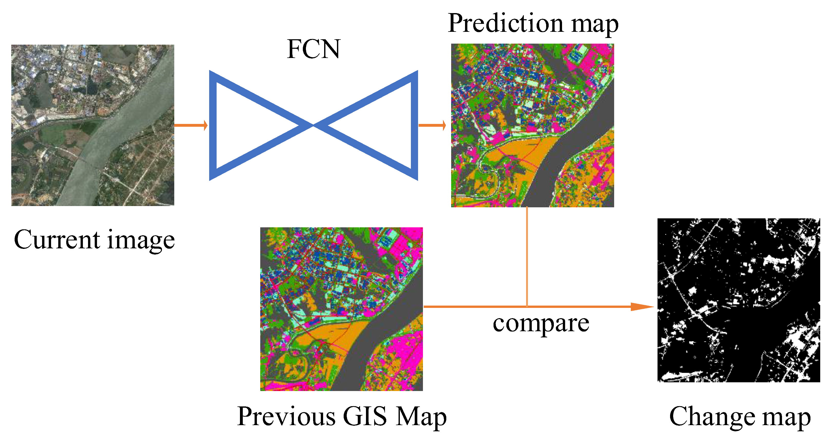
The FACNN is only executed on the current images to obtain a pixel-based classification map. A GIS map of the year 2014 (called GIS map 2014) is used as the base map. Therefore, a change map could be directly obtained by comparing the GIS map 2014 with the predicted classification map. Figure 2 illustrates this process. Firstly, the newly acquired remote sensing image is processed by the FACNN, which has been trained with the GIS map 2014 in a given training area through back propagation. The predicted segmentation map of the test area is compared to the GIS map 2014 to produce a pixel-based binary change map where white and black represent changed and unchanged pixels respectively. It is noted that as an FCN is trained on raster images and predicts a pixelwise segmentation map, the original GIS map with vector format has been preprocessed to a raster land cover map. Based upon the change map, change detection is evaluated in three levels: pixel, polygon and object level.
Pixel-based change detection. The change map in Figure 2 is already a pixel-based result of change detection. The accuracy of the change map can be strictly assessed by a reference change map, which is a changed/unchanged binary map generated by comparing the previous and current GIS maps.
Polygon-based change detection. For the polygon level change detection, we treat every polygon of the GIS map 2014 as an object instance. The pixel-wise change map in Figure 2 is seamlessly segmented by those polygons and in each polygon, when more than a certain rate of pixels was changed, we treat the object as changed.
Object-based change detection. An object-based change map is also generated from the pixel-based change map. Here an object is a patch consisting of connected change pixels (white pixels in the change map), within which if the really changed pixels exceed a given threshold, it is regarded as a correctly detected change.
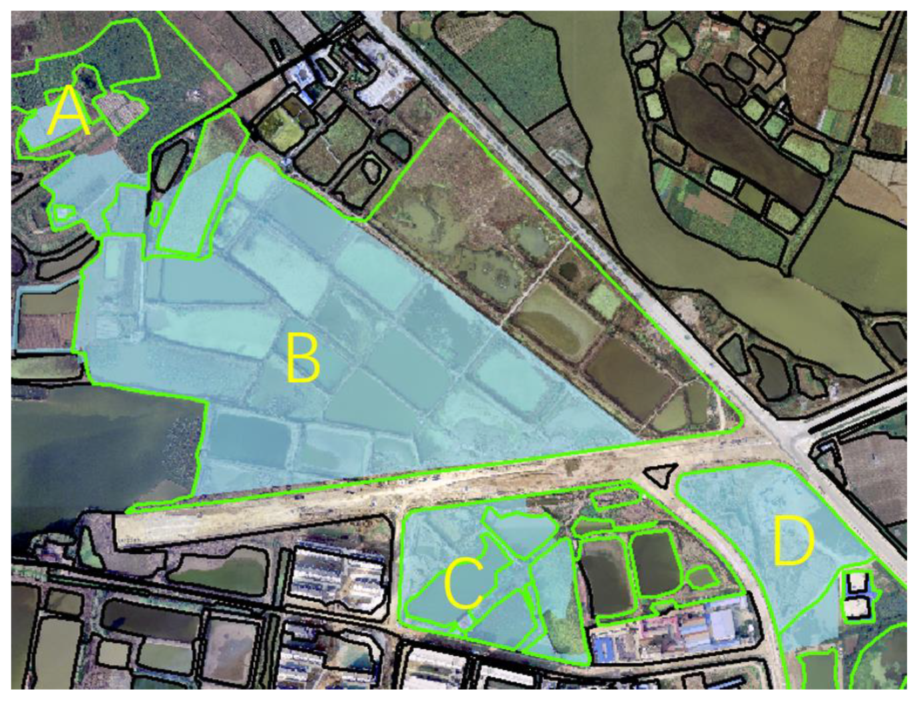
Figure 3 demonstrates the differences between the three levels of change map. The translucent blue masks retrieved from Figure 2 consist of a pixel-based change map. If a polygon contains enough change pixels, it is treated as a changed polygon (green outlines) and all of them consist of polygon-based change map. The four patches of changed pixels, A, B, C and D, consist of an object-based change map, which cover 14 changed polygons. As a large number of polygons are small and sensitive to noises, the object level change detection has the advantage of representing changes more clearly.

3. Study Site

To demonstrate the effectiveness of our method on complex and complete unban scenes, the Wuhan city is chosen as the study site. Wuhan is a large (8000 km2) and rapidly developing city located in Central China. In recent years, about 5% land covers have been changed every year, making it an ideal site to study urban land cover change detection. In this study, a land cover GIS map produced in 2014, along with its corresponding remote sensing images, is served as a base map. New remote sensing images covering the city were acquired in 2017. The changes between the 2014 GIS map and the 2017 remote sensing images are to be detected. The GIS map of 2017 is used to evaluate the performance of our classification algorithm, and the difference map between 2014 and 2017 GIS maps is used to evaluate our change detection method. The original vector GIS map has been converted to the raster land cover map.
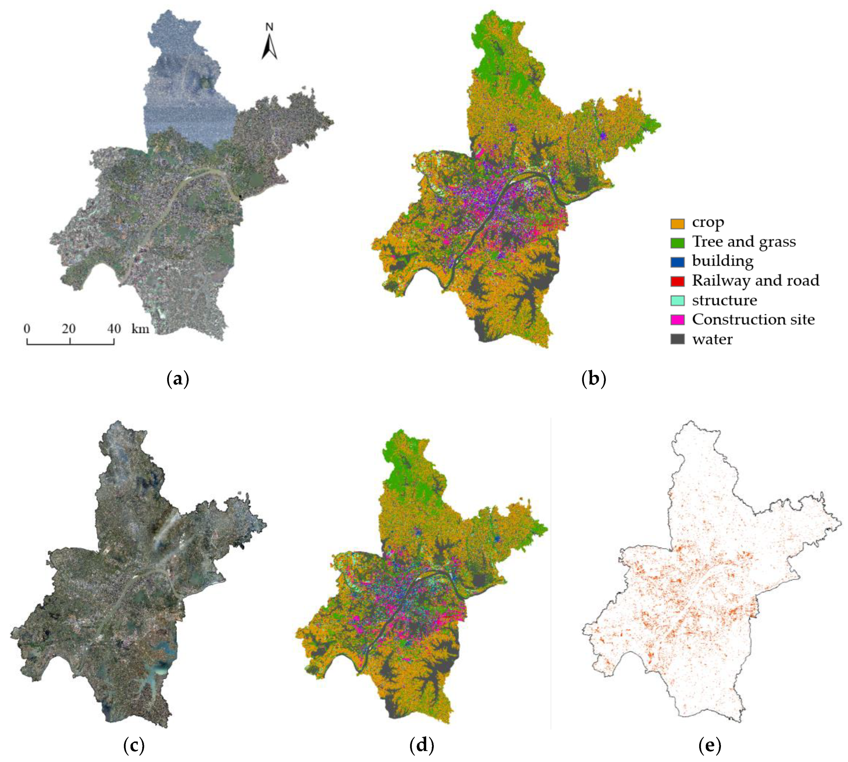
Figure 4a shows 491 stitched and geo-rectified aerial images with 0.5 m ground resolution acquired in 2014. The corresponding land cover are classified into cropland, tree and grass (vegetation), building, railway and road, structure, construction site and water (Figure 4b), according to the first level of land cover classification of China’s first national geoinformation survey.
Figure 4c shows 18 preprocessed and mosaicked Beijing-2 satellite images acquired in 2017 with 1 m ground resolution and RGB bands. Some places (top and up-right) are covered with thin cloud, which increases the difficulties in segmentation and change detection. Figure 4d shows the land cover GIS map of 2017, part of which is served as training data and the rest for testing. Figure 4e is the reference change map between Figure 4b and Figure 4d where changes are colored. The 2014 and 2017 images are registrated by georeferenced coordinates and scaled to 1 m ground resolution. The registration accuracy of most areas is about 1–2 pixels except for high buildings. However, as we focus on classification-based object-level change detection, the registration error is trivial.

4. Experiments and Results

4.1. Experimental Design

The experiments consist of two parts: a classification test including comparison with most recent methods; a change detection test that includes accuracy assessment of change maps at pixel, polygon and object level.
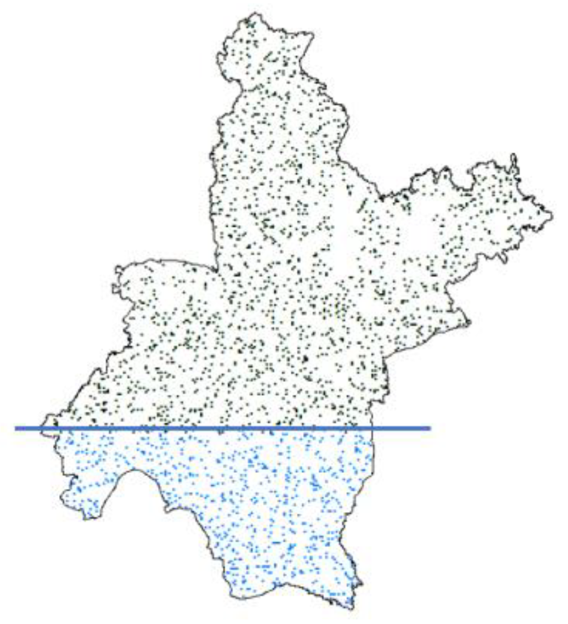
In the classification test, the classification task is divided into two stages as the data processing is computationally intensive with images covering 8000 km2 at 1 m ground resolution. In the first stage, we use adequate representative patch samples instead of the whole image for assessing the performance of different classification networks and prove the advantage of our method. In Figure 5, the 3500 512 × 512 training and validation patch samples that evenly cover the seven classes are shown in dark squares; the 700 testing samples are represented in blue squares below the line.
In the second stage, we train our FACNN on the training set and predicts on the test set (blue squares, Figure 5) for accuracy assessment. Due to the limitation of the GPU capacity, the whole image is seamlessly cropped into 23,360 512 × 512 tiles in the training area and 8577 tiles in the test area, the latter tiles after classification, are then stitched to produce a classification map, which is evaluated according to the ground truth (Figure 4d).
In the change detection test, the area predicted by the FACNN is compared to the corresponding area of the 2014 GIS map (Figure 4b) to produce a pixel-based change map, followed with polygon-based and object-based change maps.
The classification accuracy is evaluated with overall accuracy (OA) and Kappa; the accuracy of the pixel-based change detection is evaluated with OA, precision, recall and F1 score; the accuracy of the polygon and object-based change detection is evaluated with precision, recall, and omission rate.

4.2. Classificaiton Results

(1) classification with patch samples
We compared our FACNN with several representative segmentation methods that have been developed recently. In Table 1, the FCN-16 [17] is the first and baseline CNN structure for pixelwise segmentation; the U-Net [18] and Dense-Net [31] are two most widely used FCN structure; the Deeplab-v3 [19] is one of the latest algorithms that have been shown to obtain the best results with several open datasets. The four methods were developed from the machine learning community and have been applied in close-range image and remote sensing image classification. The SR-FCN [22] was developed from remote sensing community and addressed the scale effects.
Table 1 shows the predicting accuracy on the 2017 image patch samples using these segmentation networks and ours. The precision indicator in each class indicates our method considerably better in classifying crops, vegetations and construction sites. According to the overall accuracy (OA), our method outperforms the second-best algorithm by around 2%. This is mainly due to the introducing of multi-rate Atrous convolution at all scales, which helps to catch the broad scope of information and to increase the robustness against changes of different object sizes. In contrast, the FCN-16, U-Net and Dense-Net use a relatively smaller receptive field which is determined by the scaling factor of the highest semantic layer relative to the input image. This limits the algorithm’s performance in large-scale remote sensing classification. The Deeplab-v3 and SR-FCN performed better than the three methods because the ASPP was introduced into the highest semantic layer to greatly increase the receptive field. However, their lower performance relative to our method indicates that introducing the multi-rate Atrous convolutions only to the top of feature pyramid is insufficient. We introduce the Atrous convolutions to all scales of the feature pyramid, and obtained improvement in land cover classification.
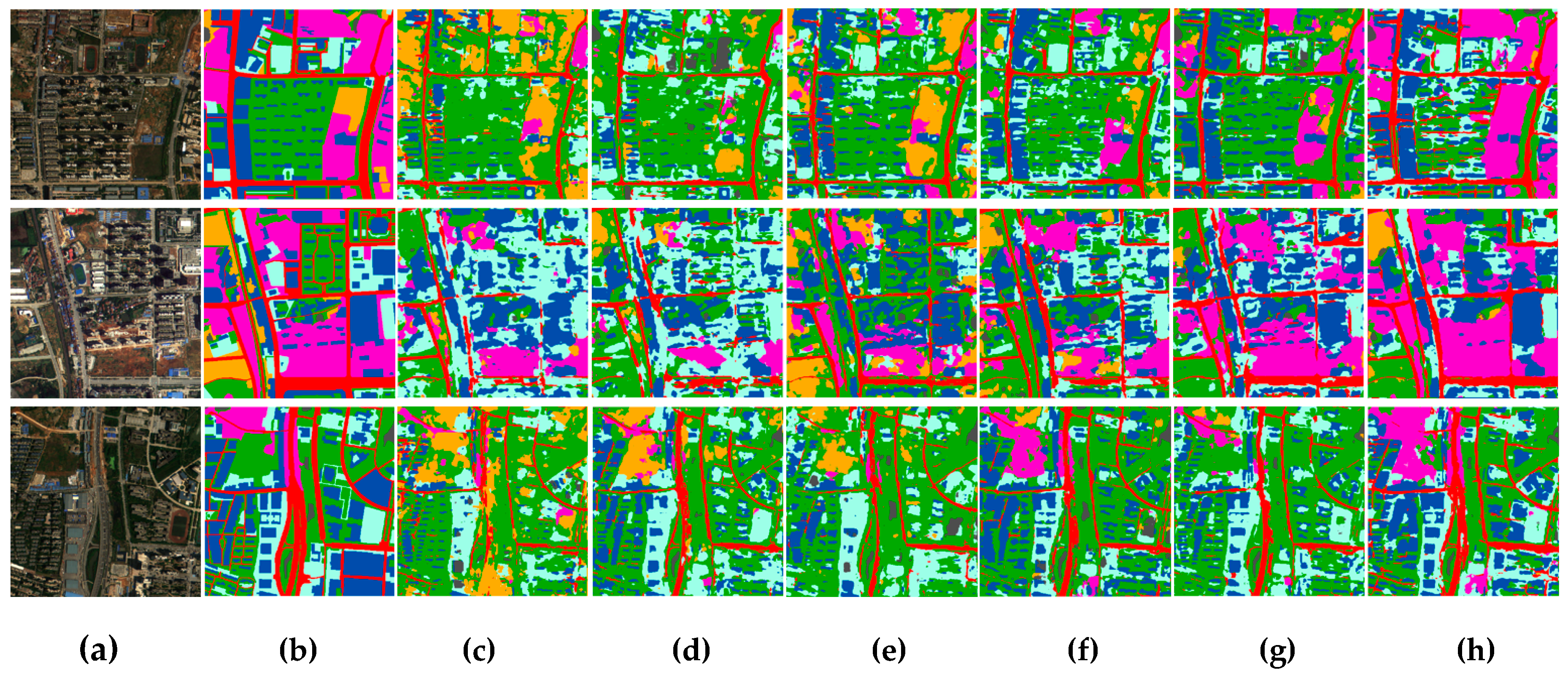
Figure 6 shows the segmentation results of different methods on three image patches. Our method performs considerably better in each patch. For example, in the upper left part of the first patch, our method could discriminate construction sites (pink), trees and grasses (green), while all other methods failed. In the second patch, the result of our method is the closest to the reference while other methods made incorrect predictions on construction sites (pink). In the third patch, the other methods consist obvious prediction errors, e.g., the FCN-16 and Dense-Net confused construction sites (pink) and vegetations (green), and the U-Net classified a considerable amount of construction sites and vegetations to crops (yellow).
Table 2 shows the confusion matrix of our method. Among all the land cover types, water is the most distinguishable object, while structure is some likely to mix with buildings (0.176), and trees and grasses are likely to be confused with crops (0.092). These findings are coincident with experience that vegetations and crops are hard to be separated especially in a mono-period RGB remote sensing image, and buildings and structures share many characteristics.
(2) Classification using the whole Wuhan data
We apply the FACNN method on the whole 2017 images. The FACNN model is pretrained on the training set to predict a classification map of the rest part (below the line). Table 3 shows the confusion matrix and precision on the test area. The overall accuracy improved from 73.2% to 76.6%, this is due to more data is used for training. Again, the most challenging problem is the confusing between vegetation and crops.
Figure 7a shows the predicted classification map using our method. It could be observed that the general characteristics of land cover types have been captured by comparing with the ground truth (Figure 4d). In the right bottom part, vegetation (green) and crop (yellow) were some mixed up. Figure 7b shows a zoomed area with 5535 × 4805 pixels (26.5 km2). Compared to the ground truth (Figure 7c) it shows the overall prediction result is satisfactory. The most obvious confusion occurred between vegetation (yellow) and crops (green) in the up-left corner and in the bottom-right corner.

4.3. Change Detection Results

(1) pixel-based change detection
A change map of the test area is produced according to a pixel-by-pixel comparison between the prediction map of our classification model (Figure 7a) and the 2014 GIS map (Figure 4b). Table 4 shows the pixel-based accuracy assessment, the F1 score is 48.5% in the changed area and 98% in the unchanged area. As the changed area only covers a minor part of the whole city, the overall accuracy reaches to 96.3%. However, in this pixel level, the recall is only 37.8%, a large number of changed regions are missed, which makes it less useful in the GIS map updating.
(2) polygon-based and object-based change detection
We calculate a polygon-based change map from the pixel-based change map by counting if the changed pixels within each polygon exceed a given minimum mapping unit (MMU) of 500 pixels.
We calculate an object-based change map by treating patches of the pixel-based map (larger than the MMU) as the unit. If more than 35% pixels within a patch are really changed, the patch is a correctly detected changed object.
On assessment, we ignore those changes less than the MMU in the ground truth map and the change detection accuracy of polygon-based and object-based approaches are listed in Table 5. We predicted 4609 changed polygons out of a total of 65,438 GIS polygons, where 4230 polygons consist of true changes. The recall and precision are 63.4% and 58.1% respectively and the omission rate is 35.6%.
1772 changed objects out of 1839 truly changed objects are detected and the corresponding recall and omission rates are 96.4% and 3.6% respectively; 620 false changed polygons are detected and the corresponding precision is 74.1%.
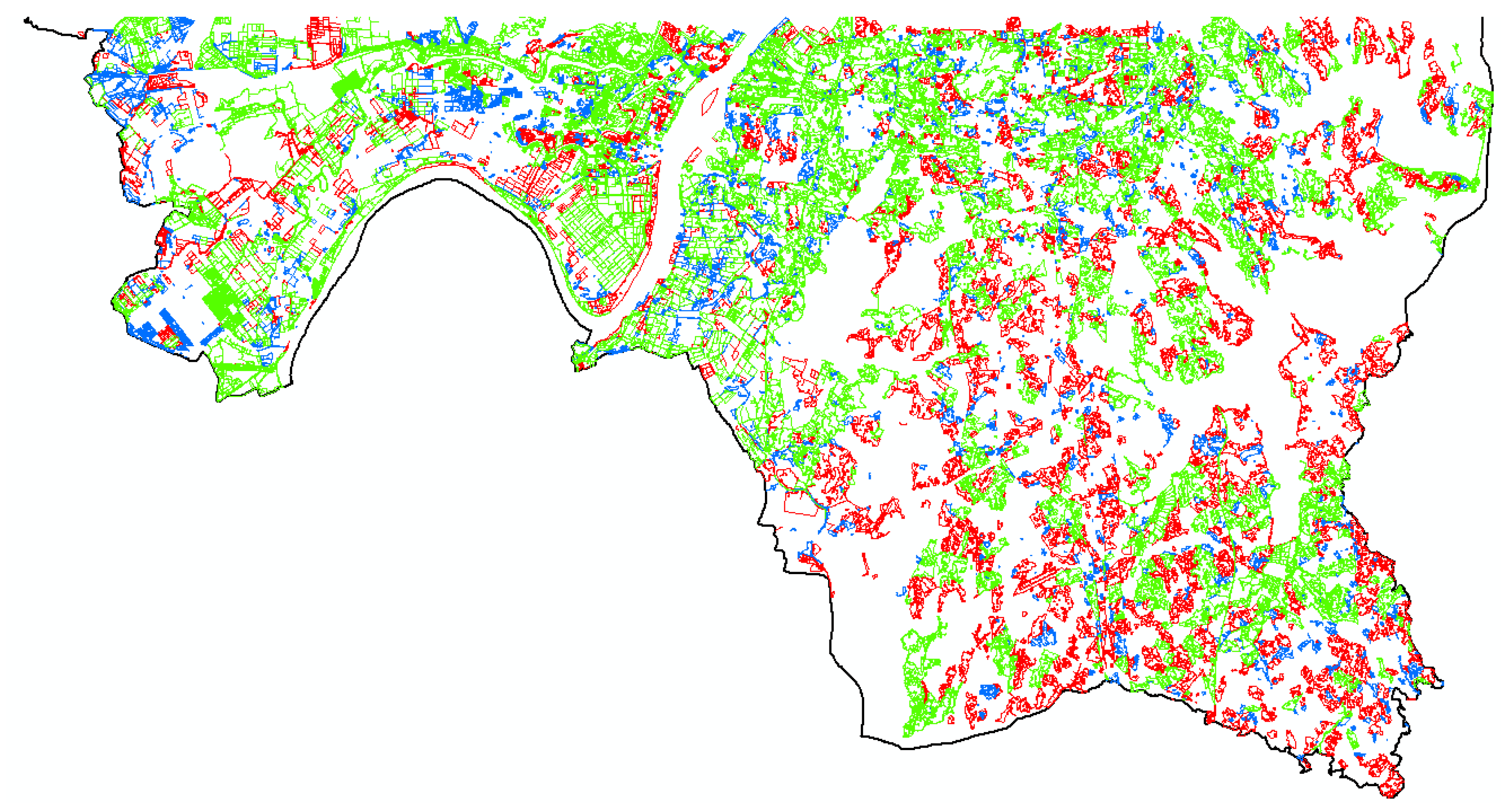
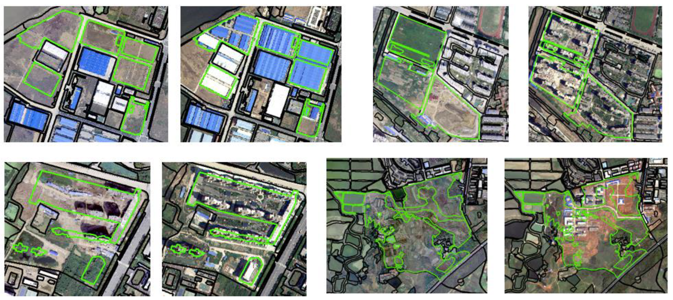
Figure 8 shows the polygon-based change map. The white background corresponds to the unchanged area that is correctly classified. Green polygons are true positives (correctly detected changed areas). Red and blue polygons are false positives (unchanged areas detected as changed wrongly, 42.9%) and false negatives (undetected changes, 36.6%) respectively. Figure 9 shows four examples of polygon-based changes that are correctly detected. Buildings were completed from crop land or construction sites. This kind of change occupies a major part of the “from-to” class changes, indicating rapid development of the city.
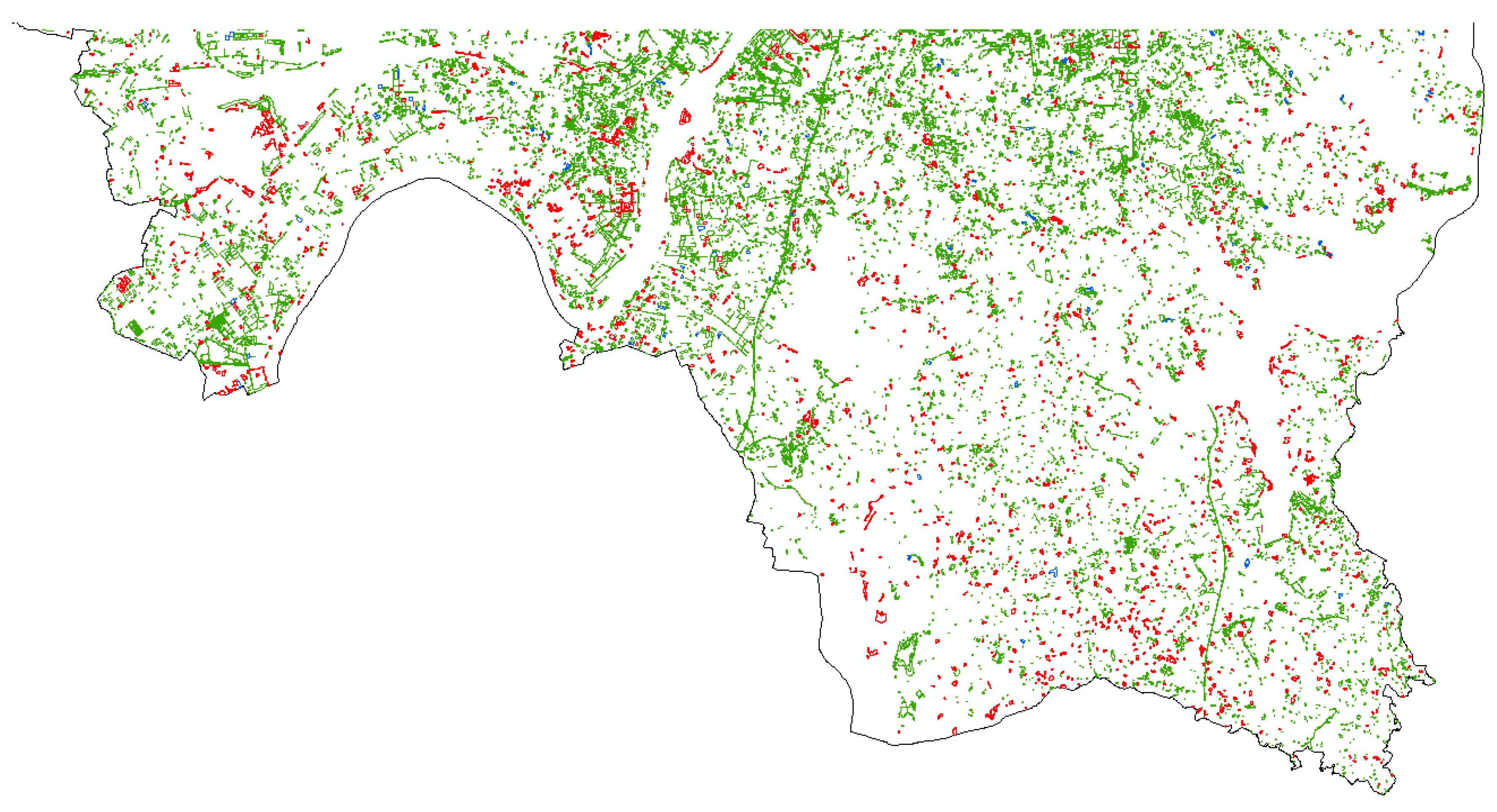
Figure 10 shows the object-based change map of our method. The white background corresponds to the unchanged area that is correctly classified. Green, red and blue objects are true positives, false positives and false negatives, respectively. Compared to the statistics on polygon, the false positives dropped and the precision improved from 58.1% to 74.1%; the false negatives (omission) dramatically dropped from 36.6% to 3.6%. This indicates that those changed pixels were often lumped together and easily detected by object-based approach but were easy to ignore by polygon based one counting on independent polygons. Basically, the object-based change map seems more accurate statistically, and the polygon-based change map is more rigorous. We will discuss this further in Section 5.

5. Discussion

In this section, we discuss practical challenges applying deep learning-based algorithm to change detection, and the different usages of the polygon-based and object-based change maps in practice.

5.1. Interpretation Inconsistency between A Deep Learning Algorthm and A Human

Interpretation inconsistency often occurs between an algorithm and an interpreter in urban land cover change detection considering the ever-changing and complex objects and backgrounds of VHR images. In particular, the changes that are negligible from a human view, sometimes known as pseudo-changes, often mislead the judgement of an algorithm.
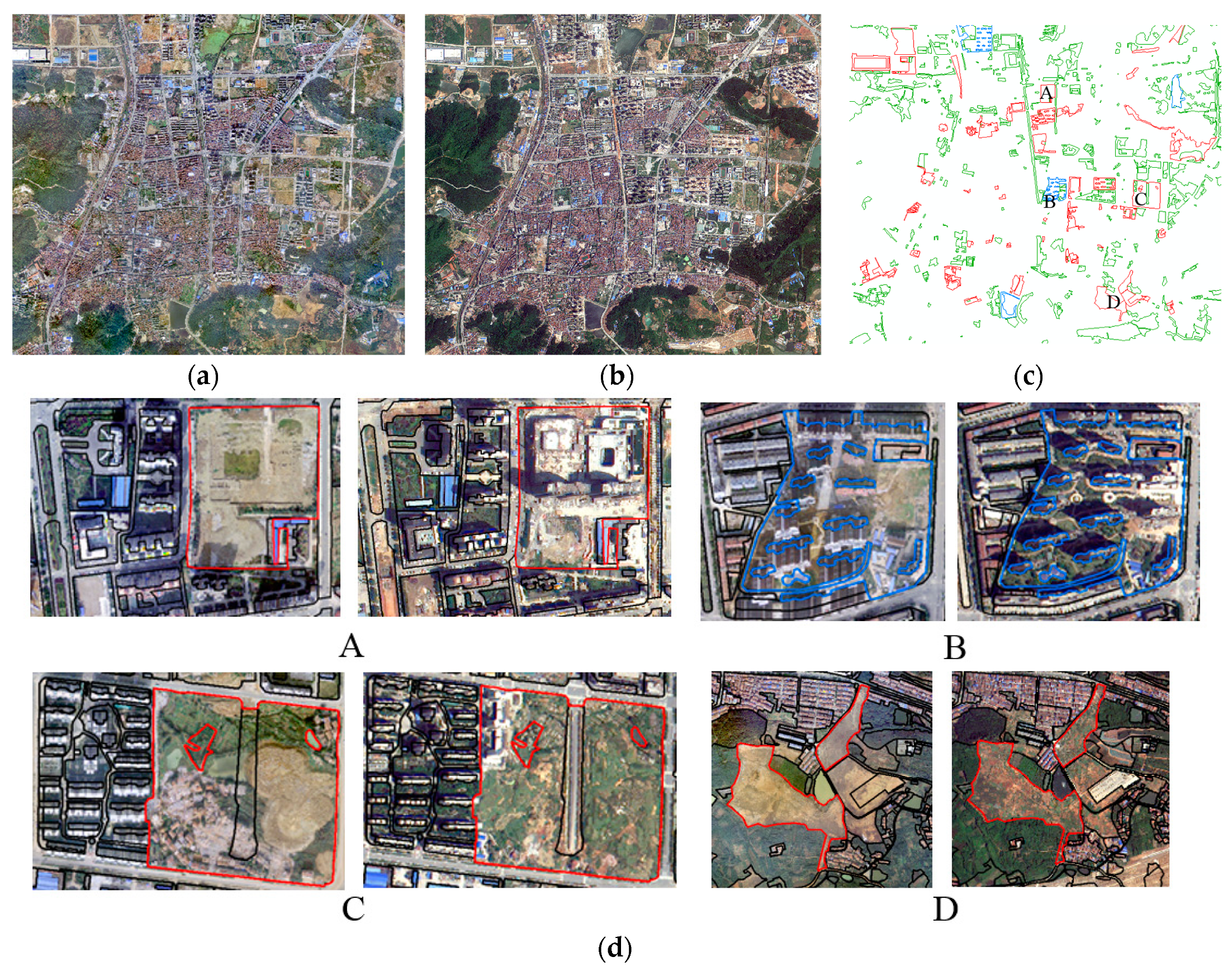
Figure 11a,b shows one rapid changing region covering 26.5 km2 and Figure 11c is the error map produced by our change detection algorithm where true positives, false positives and false negatives were denoted by green, red and blue polygons, respectively. Area A (Figure 11d) shows a challenging scene for most of the change detection algorithms. An unchanged construction site (by interpreter judgement) was classified to buildings in the new image by the algorithm. The large uncompleted buildings that are under construction standing on a bare ground at the right corner lead to the wrong judgement of the algorithm. In the area B, a construction site (denoted by the largest blue polygon excluding the inner building polygons) has been changed into buildings. Our algorithm has successfully detected two new buildings in the right part, but they were treated as an unchanged polygon as the area is less than 500 pixels. The three unchanged polygons (judged by interpreter) in the area C (construction sites) were classified into structures and vegetation by the algorithm, because a large area of grassland appearing on the bare land. Similarly, the manually interpreted unchanged construction sites in the D area were classified into crops and vegetation by the algorithm.
Figure 12 shows a regional interpretation inconsistency between an interpreter and an algorithm. Paddy is a major type of crops in Wuhan city. In the new image (Figure 12c), paddy fields were filled with water in early summer and are classified into water (Figure 12e) by a “successful” application of the algorithm, which result in a classification error from human judgement.
The above cases show the algorithms have correctly detected the changes but tagged them incorrectly due to anthropogenic activities or human commonsense. This implies the next step of achieving a higher level of automation is to introduce empirical rules to an end-to-end deep learning framework and bridge gaps between human and algorithm interpretation inconsistency. For example, a simple rule that treats those cropland-to-water changes as unchanged in certain crop area could be imbedded in the algorithm.

5.2. Usage of Polygon-Based and Object-Based Change Maps

This study has developed a large-scale VHR urban image classification procedure and showed how it could be used in change detection. Here we discuss different usages of the two object-based change maps from a practical view. The polygon-based change map is used as the base map for analyzing performance and problems of the algorithm. The analysis and discussion of Figure 9, Figure 11 and Figure 12 are all polygon-based. The polygon-based accuracy indicators are accurate and rigorous, and no empirical parameters and thresholds are required except an MMU.
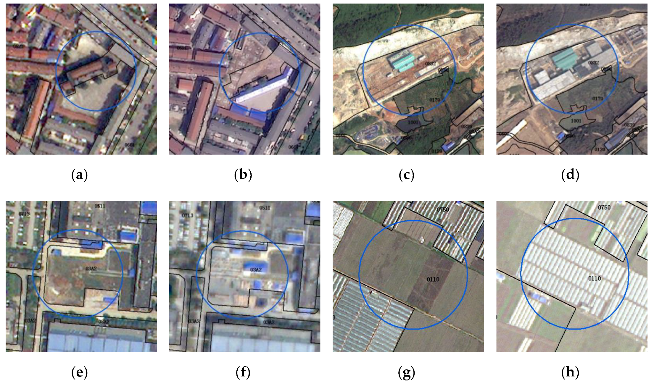
The object-based change map, with a very high recall rate of changed area, is a product that is transferred to GIS map cartographers for quick manual updating. Although one parameter, i.e., the percentage of true changed pixels among a predicted changed patch, is required to set, which lead to unreliable accuracy assessment, an object-based approach is capable of supplying a change map of a much higher recall rate than the polygon-based approach and locating those main changed regions quickly, as well as discovering those changed regions missed by human interpretation. Figure 13 shows examples where the algorithm found a changed area that is missed by human interpretation.

6. Conclusions

This study investigated the applications of the CNN-based methods to large-scale urban land cover classification and change detection from VHR remote sensing imagery. An FCN-based segmentation algorithm imbedded with multi-scale Atrous convolutions is introduced and is proved to be robust to objects with different scales, and is superior to other classic FCN methods in terms of the classification accuracy. Based on the classification results of current remote sensing images and an available historical GIS map, change maps are made and the accuracy is assessed at different levels (i.e., pixel, polygon, and object levels). Experimental results show highly accurate change maps could be achieved at the object level, this finding is valuable for GIS map updating.
The study site covers a complete, complex and rapid developing city, which is an ideal place for studying change detection methodologies as large areas with enough changes guaranteed very good statistical significance. Our method could easily be extended to other change detection cases using optical remote sensing data as we only used RGB bands, which are always available with VHR satellite and aerial images. We also found empirical rules designing is necessary to compensate the deficiency of an end-to-end deep learning-based method and to bridge the gaps between human and algorithm interpretation.

Author Contributions

Chi Zhang and Shiqing Wei prepared the data and performed the experiments; Shunping Ji led the research, analyzed the results and wrote the paper; Meng Lu involved in experiment designing and revised the paper.

Acknowledgments

This work was supported by the project of Land Cover Change Detection of Wuhan City from the Wuhan Institute of Surveying and Mapping. The algorithm has been successfully applied to the 2018 annual GIS map updating of Wuhan city.

Conflicts of Interest

The authors declare no conflict of interest.

References

  1. Walter, V. Object-based classification of remote sensing data for change detection. ISPRS J. Photogramm. Remote Sens. 2004, 58, 225–238. [Google Scholar] [CrossRef]
  2. Desclée, B.; Bogaert, P.; Defourny, P. Forest change detection by statistical object-based method. Remote Sens. Environ. 2006, 102, 1–11. [Google Scholar] [CrossRef]
  3. Stow, D. Geographic object-based image change analysis. In Handbook of Applied Spatial Analysis; Springer: Berlin, Germany, 2010; pp. 565–582. [Google Scholar]
  4. Gamanya, R.; De Maeyer, P.; De Dapper, M. Object-oriented change detection for the city of Harare, Zimbabwe. Expert Syst. Appl. 2009, 36, 571–588. [Google Scholar] [CrossRef]
  5. Nemmour, H.; Chibani, Y. Multiple support vector machines for land cover change detection: An application for mapping urban extensions. ISPRS J. Photogramm. Remote Sens. 2006, 61, 125–133. [Google Scholar] [CrossRef]
  6. Coppin, P.; Jonckheere, I.; Nackaerts, K.; Muys, B.; Lambin, E. Review ArticleDigital change detection methods in ecosystem monitoring: A review. Int. J. Remote Sens. 2004, 25, 1565–1596. [Google Scholar] [CrossRef]
  7. Todd, W.J. Urban and regional land use change detected by using Landsat data. J. Res. US Geol. Surv. 1977, 5, 529–534. [Google Scholar]
  8. Zhang, C.; Sargent, I.; Pan, X.; Li, H.; Gardiner, A.; Hare, J.; Atkinson, P.M. An object-based convolutional neural network (OCNN) for urban land use classification. Remote Sens. Environ. 2018, 216, 57–70. [Google Scholar] [CrossRef]
  9. Paris, C.; Bruzzone, L.; Fernandez-Prieto, D. A Novel Approach to the Unsupervised Update of Land-Cover Maps by Classification of Time Series of Multispectral Images. IEEE Trans. Geosci. Remote Sens. 2019, 1–19. [Google Scholar] [CrossRef]
  10. Shackelford, A.K.; Davis, C.H. A combined fuzzy pixel-based and object-based approach for classification of high-resolution multispectral data over urban areas. IEEE Trans. Geosci. Remote Sens. 2003, 41, 2354–2363. [Google Scholar] [CrossRef]
  11. Wardlow, B.; Egbert, S.; Kastens, J. Analysis of time-series MODIS 250 m vegetation index data for crop classification in the U.S. Central Great Plains. Remote Sens. Environ. 2007, 108, 290–310. [Google Scholar] [CrossRef] [Green Version]
  12. Conrad, C.; Colditz, R.R.; Dech, S.; Klein, D.; Vlek, P.L.G. Temporal segmentation of MODIS time series for improving crop classification in Central Asian irrigation systems. Int. J. Remote Sens. 2011, 32, 8763–8778. [Google Scholar] [CrossRef]
  13. Ruiz, L.; Fdez-Sarría, A.; Recio, J. Texture feature extraction for classification of remote sensing data using wavelet decomposition: A comparative study. In Proceedings of the 20th ISPRS Congress, Istanbul, Turkey, 12–23 July 2004; pp. 1109–1114. [Google Scholar]
  14. Garzelli, A.; Zoppetti, C. Urban Footprint from VHR SAR Images: Toward a Fully Operational Procedure. In Proceedings of the IGARSS 2018 IEEE International Geoscience and Remote Sensing Symposium, Valencia, Spain, 22–27 July 2018; pp. 6083–6086. [Google Scholar]
  15. LeCun, Y.; Bengio, Y.; Hinton, G. Deep learning. Nature 2015, 521, 436–444. [Google Scholar] [CrossRef] [PubMed]
  16. Kemker, R.; Salvaggio, C.; Kanan, C. Algorithms for semantic segmentation of multispectral remote sensing imagery using deep learning. ISPRS J. Photogramm. Remote Sens. 2018, 145, 60–77. [Google Scholar] [CrossRef] [Green Version]
  17. Long, J.; Shelhamer, E.; Darrell, T. Fully convolutional networks for semantic segmentation. In Proceedings of the 2015 IEEE Conference on Computer Vision and Pattern Recognition, Boston, MA, USA, 7–12 June 2015; pp. 3431–3440. [Google Scholar]
  18. Ronneberger, O.; Fischer, P.; Brox, T. U-net: Convolutional networks for biomedical image segmentation. In Proceedings of the 2015 International Conference on Medical Image Computing and Computer-Assisted Intervention, Munich, Germany, 5–9 October 2015; pp. 234–241. [Google Scholar]
  19. Chen, L.-C.; Papandreou, G.; Kokkinos, I.; Murphy, K.; Yuille, A.L. DeepLab: Semantic Image Segmentation with Deep Convolutional Nets, Atrous Convolution, and Fully Connected CRFs. IEEE Trans. Pattern Anal. Mach. Intell. 2018, 40, 834–848. [Google Scholar] [CrossRef] [Green Version]
  20. Lin, T.-Y.; Dollár, P.; Girshick, R.; He, K.; Hariharan, B.; Belongie, S. Feature pyramid networks for object detection. arXiv, 2017; arXiv:1612.03144. [Google Scholar]
  21. Ji, S.; Wei, S.; Lu, M. Fully Convolutional Networks for Multisource Building Extraction from an Open Aerial and Satellite Imagery Data Set. IEEE Trans. Geosci. Remote Sens. 2018, 57, 574–586. [Google Scholar] [CrossRef]
  22. Ji, S.; Wei, S.; Lu, M. A scale robust convolutional neural network for automatic building extraction from aerial and satellite imagery. Int. J. Remote Sens. 2018, 40, 3308–3322. [Google Scholar] [CrossRef]
  23. Yu, F.; Koltun, V. Multi-scale context aggregation by dilated convolutions. arXiv, 2015; arXiv:1511.07122. [Google Scholar]
  24. Chen, L.-C.; Papandreou, G.; Schroff, F.; Adam, H. Rethinking atrous convolution for semantic image segmentation. arXiv, 2017; arXiv:1706.05587. [Google Scholar]
  25. Wang, P.; Chen, P.; Yuan, Y.; Liu, D.; Huang, Z.; Hou, X.; Cottrell, G. Understanding convolution for semantic segmentation. In Proceedings of the 2018 IEEE Winter Conference on Applications of Computer Vision (WACV), Lake Tahoe, NV, USA, 12–15 March 2018; pp. 1451–1460. [Google Scholar]
  26. Guo, R.; Liu, J.; Li, N.; Liu, S.; Chen, F.; Cheng, B.; Duan, J.; Li, X.; Ma, C. Pixel-Wise Classification Method for High Resolution Remote Sensing Imagery Using Deep Neural Networks. ISPRS Int. J. Geo-Inf. 2018, 7, 110. [Google Scholar] [CrossRef]
  27. Lunetta, R.S.; Knight, J.F.; Ediriwickrema, J.; Lyon, J.G.; Worthy, L.D. Land-cover change detection using multi-temporal MODIS NDVI data. Remote Sens. Environ. 2006, 105, 142–154. [Google Scholar] [CrossRef]
  28. Du, Y.; Teillet, P.M.; Cihlar, J. Radiometric normalization of multitemporal high-resolution satellite images with quality control for land cover change detection. Remote Sens. Environ. 2002, 82, 123–134. [Google Scholar] [CrossRef]
  29. Nair, V.; Hinton, G.E. Rectified linear units improve restricted boltzmann machines. In Proceedings of the 27th International Conference on Machine Learning (ICML-10), Haifa, Israel, 21–24 June 2010; pp. 807–814. [Google Scholar]
  30. Ioffe, S.; Szegedy, C. Batch normalization: Accelerating deep network training by reducing internal covariate shift. arXiv, 2015; arXiv:1502.03167. [Google Scholar]
  31. Huang, G.; Liu, Z.; Maaten, L.V.D.; Weinberger, K.Q. Densely Connected Convolutional Networks. In Proceedings of the IEEE Conference on Computer Vision and Pattern Recognition, Honolulu, HI, USA, 21–26 July 2017; pp. 2261–2269. [Google Scholar]
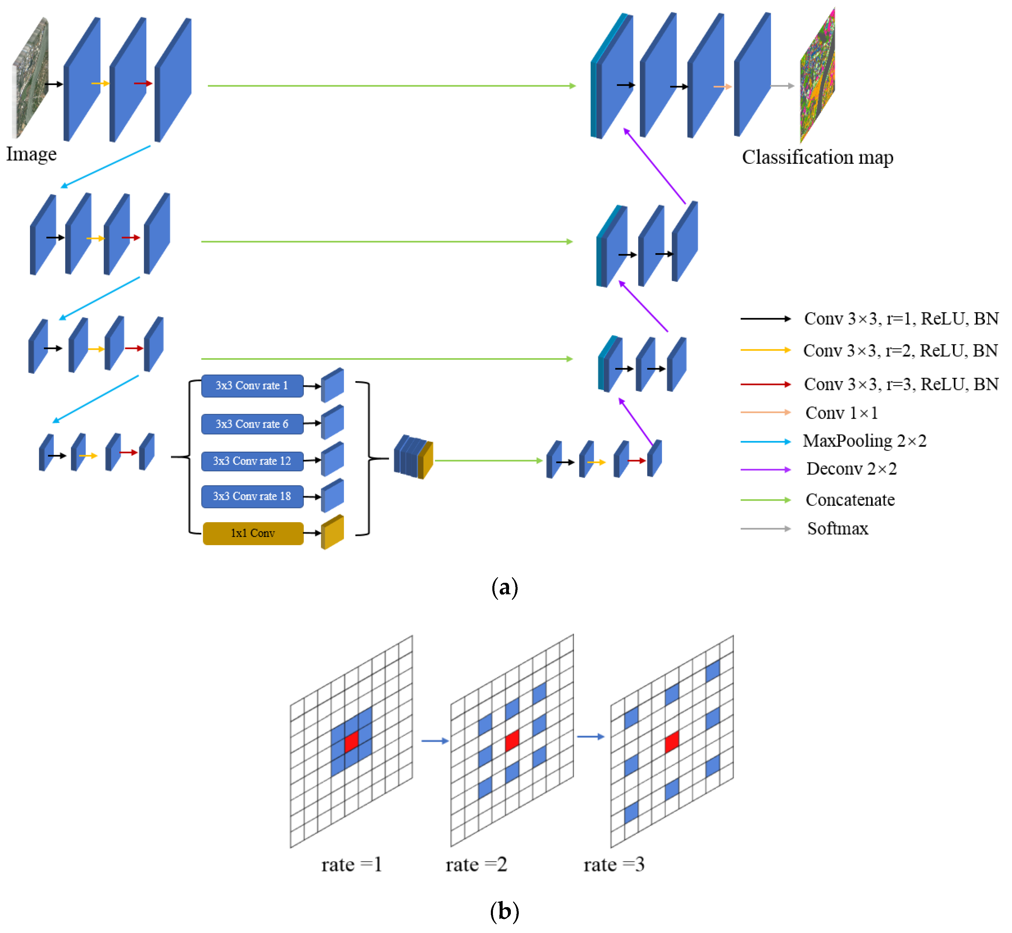
Figure 1. Our FACNN structure for land use segmentation. Multi-rate Atrous convolution is introduced into each scale of the encoder, and in the highest scale an ASPP is added (a). (b) shows the different rates of sequential Atrous convolution where red pixel is the kernel center and blue and red consist of a kernel. The white pixels are skipped.
Ijgi 08 00189 g001
Figure 2. The structure for change detection. The FACNN is used to extract a segmentation map from the new image. The segmentation map is compared to the GIS map 2014 to produce a pixelwise change map.
Ijgi 08 00189 g002
Figure 3. A demonstration of a change map at pixel, polygon and object level. The translucent blue masks show changes at the pixel level. The black borderline polygons are the unchanged regions; the 14 green polygons overlap with the changed pixels exceeding a certain overlapping percent are changed polygons. Those connected change pixels in the pixel-based map are grouped into a changed “object”. There are A, B, C and D four patches changed at the object level.
Ijgi 08 00189 g003
Figure 4. The 2014 Wuhan aerial images covering 8000 km2 with 0.5 m ground resolution (a) and the corresponding land cover GIS map (b). The 2017 Beijing-2 satellite images with 1 m ground resolution (c) and the corresponding land cover GIS map (d). (e) is the ground truth of change map produced from comparing Figure 1b,d.
Ijgi 08 00189 g004
Figure 5. In the first classification stage, 4200 512 × 512 patch samples retrieved from the 2017 image are used for evaluating different algorithms’ performance, where the 3500 black rectangles above the line are training and validation data and the 700 blue ones below the line are test data. In the second stage, all the image pixels above the line are used for training and the rest for testing.
Ijgi 08 00189 g005
Figure 6. Classification results of different FCN structures. (a) and (b) are the images and ground truth, (ch) are the results of FCN-16, U-Net, Dense-Net, Deeplab-v3, SR-FCN and ours.
Ijgi 08 00189 g006
Figure 7. (a) The prediction results of land use classification using our FACNN network; (b) a zoomed area with 5535 × 4805 pixels; (c) the ground truth of the zoomed area.
Ijgi 08 00189 g007
Figure 8. The polygon-based change map, where the white background is unchanged area, green polygons are correctly detected changed polygons, red and blue are false positives and false negatives.
Ijgi 08 00189 g008
Figure 9. Four examples of polygon-based change maps. Green polygons overlaid on the 2014 and 2017 images present the detected change areas where true changes underwent. Black polygons are those unchanged areas.
Ijgi 08 00189 g009
Figure 10. The object-based change map, where the white background is the unchanged area, green polygons are correctly detected changed objects, red and blue indicate respectively false positives and false negatives.
Ijgi 08 00189 g010
Figure 11. The zoomed-in area with 5535 × 4805 pixels. (a) image in 2014; (b) image in 2017; (c) the polygon-based change map, where the white background is the unchanged area, green polygons are correctly detected changed objects, red and blue are false positive and false negative; (d) four zoom-in area. A, C and D are unchanged construction sites that were wrongly classified into buildings, plants and constructions, plants and crops, respectively. B is a missing detected polygon where the right part of the construction site has been changed into buildings.
Ijgi 08 00189 g011
Figure 12. A case of human and algorithm interpretation inconsistency. Image in 2014 (a) and in 2017 (c) were both classified to cropland (yellow) by human as ground truth (b) and (d). However, a large part of area was classified into water by the algorithm (e) because of the irrigation season of paddy.
Ijgi 08 00189 g012
Figure 13. The circled polygons are changed objects missed by a cartographer but detected by the algorithm. From (af), the cartographer slipped up probably due to the complex environments and unobtrusive changes; in (g) and (h), the mistake is caused by obsolescence of knowledge: before 2016 green house is classified to crop land but thereafter is classified to constructions according to the rule of China’s first national geoinformation survey.
Ijgi 08 00189 g013
Table 1. The precision and overall accuracy of the FCN-16, U-Net, Dense-Net, Deeplab-v3, SR-FCN and our method on the 2017 patch samples.
MethodCropVegetationBuildingRailway and RoadStructureConstruction SiteWaterKappaOA
FCN-160.6060.5310.7190.6670.6610.6320.8830.6660.655
U-Net0.6470.5940.7220.7110.6780.7170.8880.7040.695
Dense-Net0.6640.6050.7480.6780.7090.6910.8840.7110.702
Deeplabv30.6730.6270.7400.7420.6860.7150.8850.7200.711
SR-FCN0.6630.6100.7610.7760.7140.7080.8890.7230.713
Ours0.6850.6280.7790.7860.7560.7200.8960.7410.732
Table 2. The confusion matrix of our method on the patch samples.
TypeCropTree and GrassBuildingRailway and RoadStructureConstruction SiteWater
Crop0.7230.1110.0110.0120.0330.0790.031
Tree and grass0.1070.7530.0260.0180.0060.0580.032
building0.0160.0850.7960.0120.0580.0290.004
Railway and road0.0480.0370.0750.6780.0780.0710.013
structure0.0720.0890.0820.0240.6450.0710.017
Construction site0.0440.0950.0620.0370.0260.7300.006
water0.0710.0560.0070.0080.0210.0090.828
Overall Accuracy = 0.732; Kappa = 0.741
Table 3. The confusion matrix, OA and Kappa of our method on the test area.
TypeCropTree and GrassBuildingRailway and RoadStructureConstruction SiteWater
Crop0.7180.1470.0060.0070.0330.0300.059
Tree and grass0.0860.6260.0680.0580.0630.0680.031
Building0.0110.0540.8030.0210.0610.0500.001
Railway and road0.0330.0720.0370.7430.0590.0510.007
Structure0.0530.0770.2040.0980.4950.0620.010
Construction site0.0740.0520.0520.0280.0390.7320.023
Water0.0470.0530.0020.0020.0060.0080.880
Precision0.7030.5790.6860.7760.6550.7320.870
Overall Accuracy = 0.766; Kappa = 0.744
Table 4. The change detection accuracy in pixel level.
PixelPrecisionRecallF1 Score
unchanged0.9820.9780.980
changed0.6770.3780.485
Overall Accuracy = 0.963; Kappa = 0.329
Table 5. The change detection accuracy assessed on polygon and object level. GT indicates those truly changed polygons/objects retrieved from the difference map between 2014 and 2017 GIS maps.
TypeNumberGTPredictedRecallPrecisionOmissionF1
Polygon65,4384230460963.4%58.1%36.6%60.6%
object/1839239296.4%74.1%3.6%83.8%