Registration of Multi-Sensor Bathymetric Point Clouds in Rural Areas Using Point-to-Grid Distances

 ,
, 
Abstract
:1. Introduction
2. State of the Art
3. Method
| Algorithm 1: Algorithm overview. |
| Data: LiDAR and Photogrammetric point cloud Result: transformation parameters G = calculate DEM(LiDAR); t = initial threshold; M = initialize Model(); 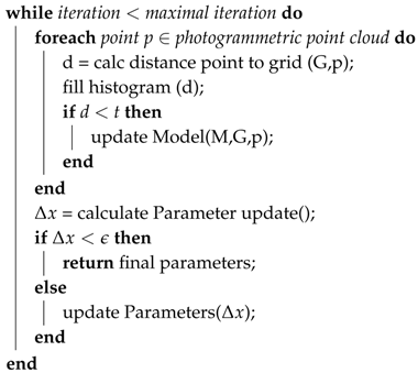 |
3.1. The Minimizing of Point to DEM Distances
- s = x − xi difference inside the range [0, 1] of the x coordinate of the current point to the x coordinate of the anchor edge (xi) on the grid.
- t = y − yj: analogue to s with the y coordinates of the current point.
- a = heights of the grid cells edge points (i.e., estimated grid parameter).
- i,j = coordinates of the anchor edge of the current grid cell, corresponding to the given x, y values.
- = coordinates of the point k.
- = weight for point k to the cell’s edge l.
- = coordinates of the cell’s edge l.
- = grid parameter corresponding to the cell’s edge l.
- N = neighborhood of considered points.
- = translation along x, y, z-axis.
- = coordinates of the point to be transformed.
- m = scale.
- = rotation with the Euler angles .
- = vector of the parameters e.g., .
- = functional matrix (derivatives of the observation functions (Equation (6)) with respect to the parameters ) = .
- = matrix of conditional observations (derivatives of the observation functions (Equation (6)) with respect to the coordinates of ) = .
- Q = covariance matrix of observations (i.e., stochastic model).
- f = vector of for each point.
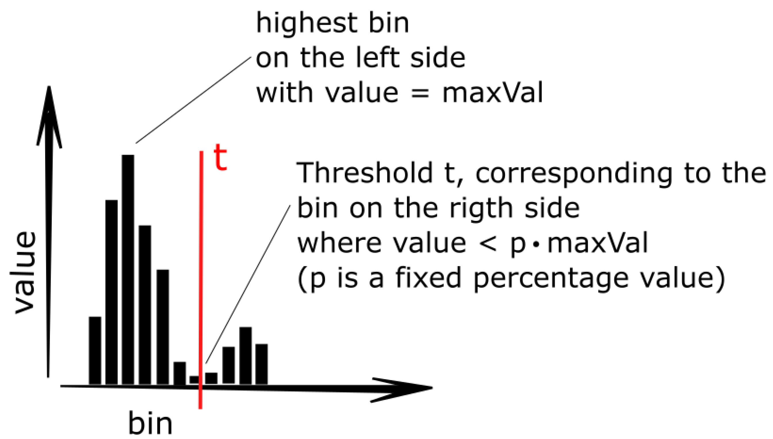
3.2. Outlier Removal
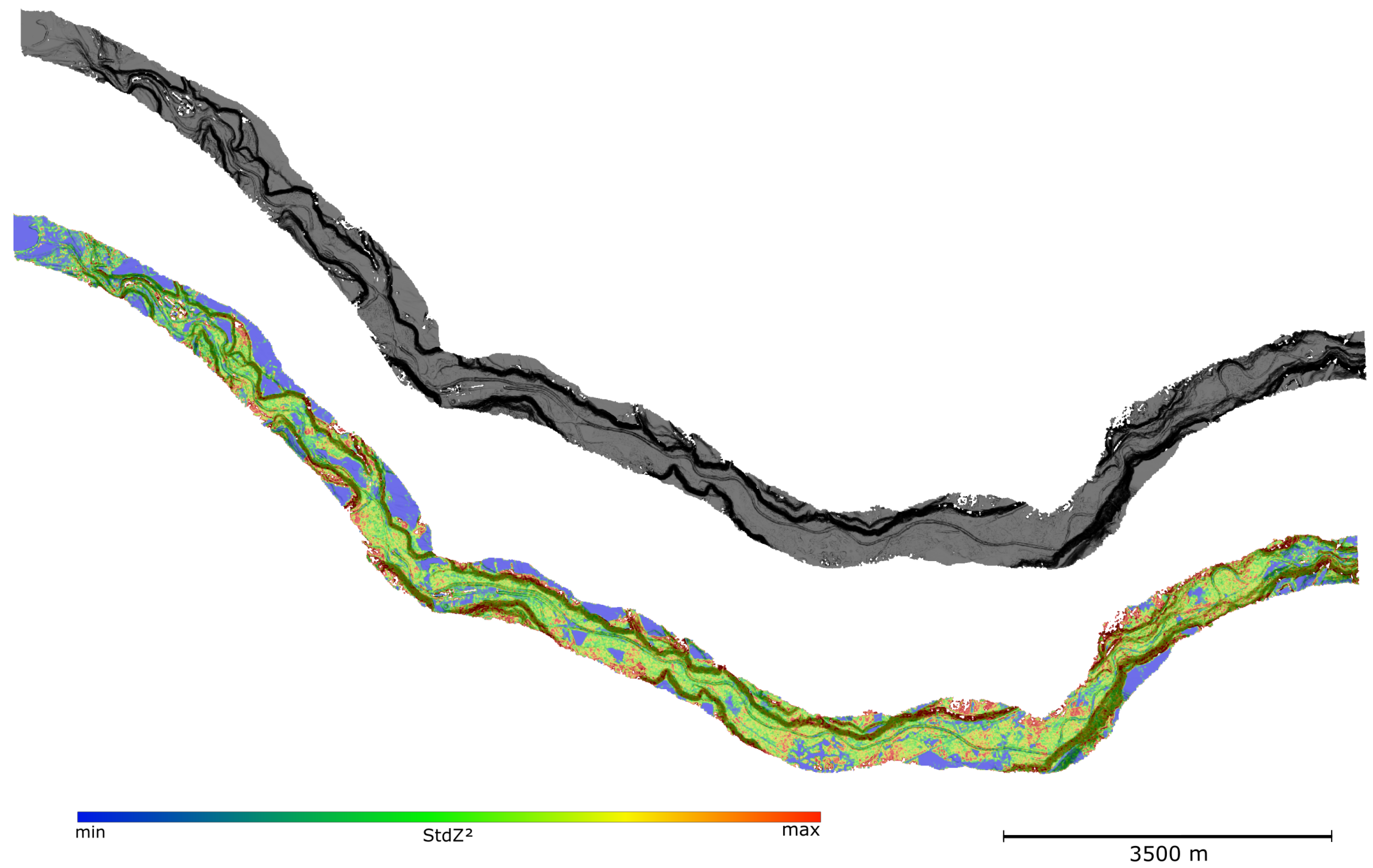
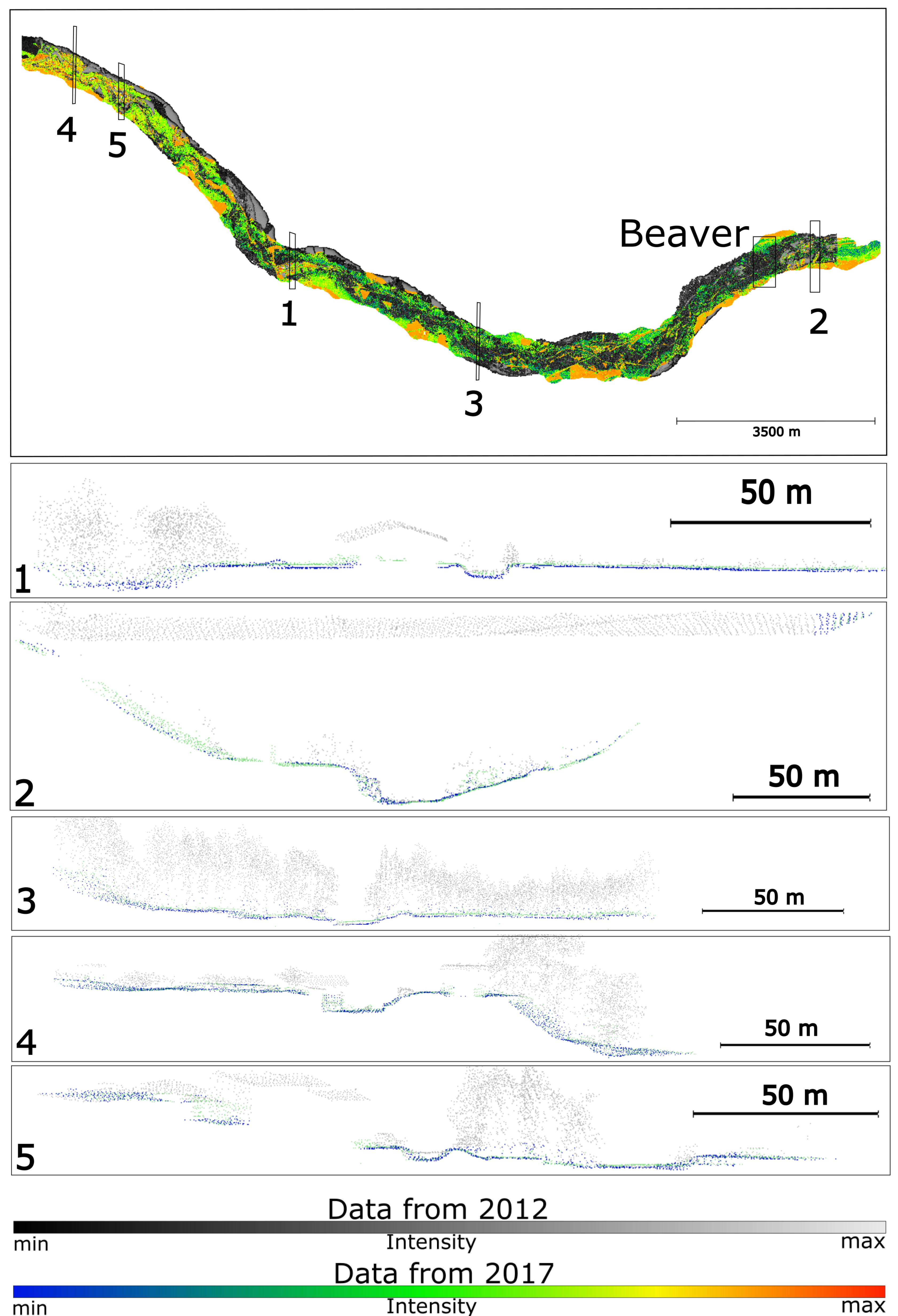
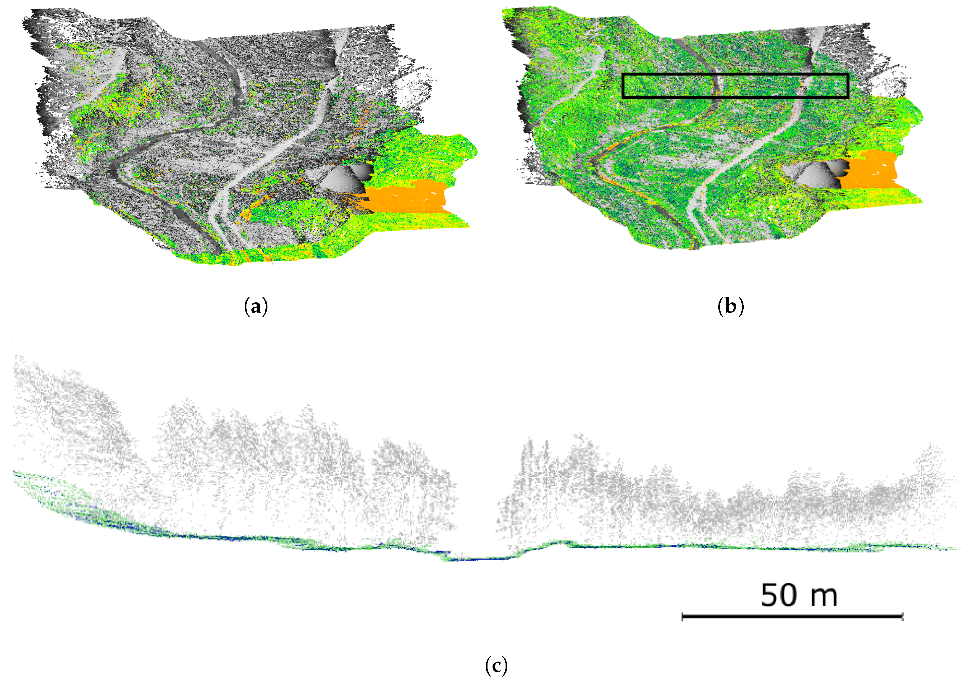
4. Data
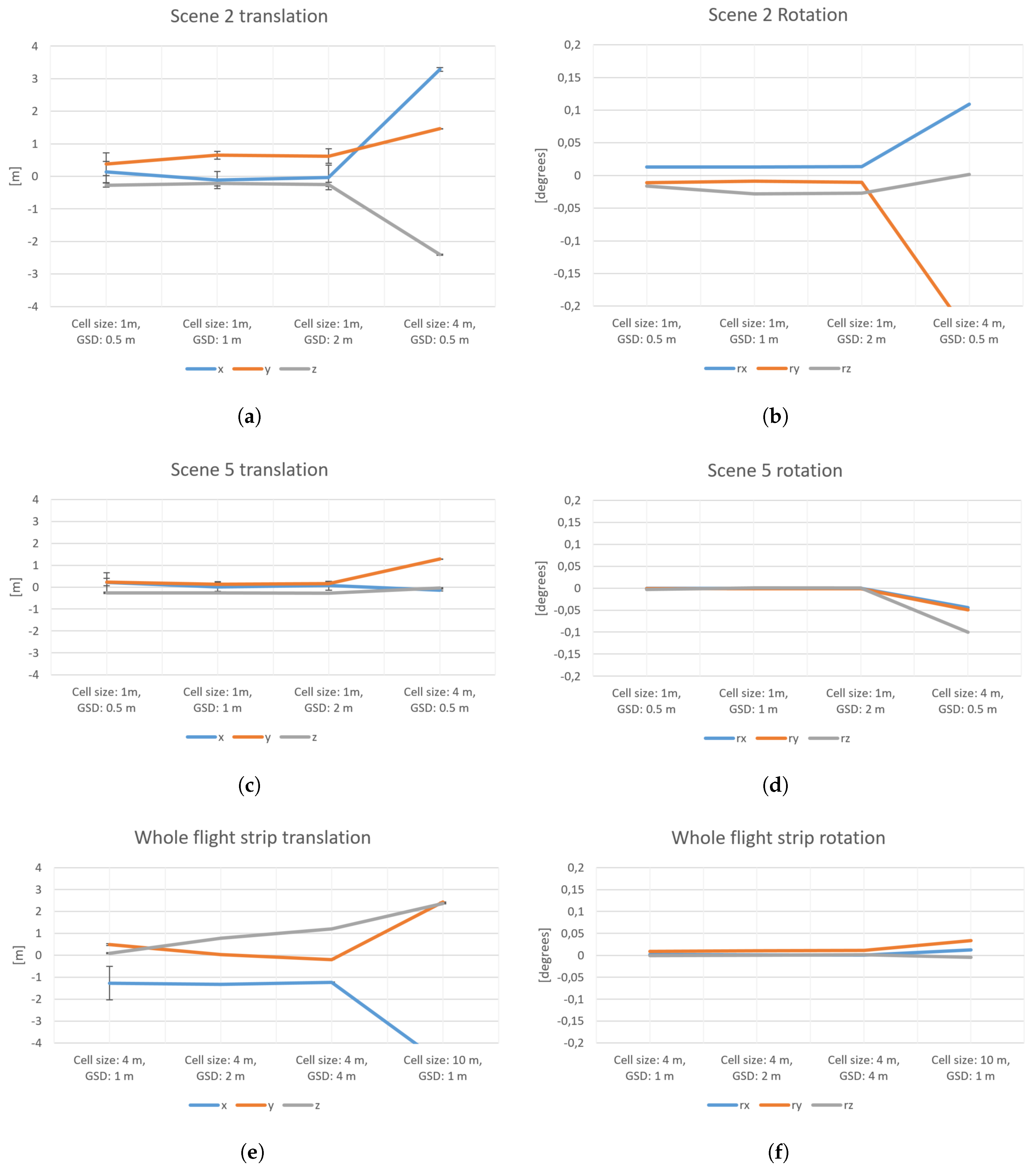
5. Results
5.1. Description of Experiments
5.2. Results of Experiments
6. Discussion
6.1. Discussion of Results and Comparison with Other Work
6.2. Limitation and Future Direction
7. Conclusions
Author Contributions
Funding
Acknowledgments
Conflicts of Interest
Abbreviations
| MDPI | Multidisciplinary Digital Publishing Institute |
| GSD | Ground-Sampling Distance |
| DEM | Digital Elevation Model |
References
- Besl, P.J.; McKay, N.D. Method for registration of 3-D shapes. In Robotics-DL Tentative; International Society for Optics and Photonics: Bellingham, WA, USA, 1992; pp. 586–606. [Google Scholar]
- Boerner, R.; Xu, Y.; Hoegner, L.; Baran, R.; Steinbacher, F.; Stilla, U. DEM based registration of multi-sensor airborne point clouds exemplary shown on a river side in non urban area. Int. Arch. Photogramm. Remote Sens. Spat. Inf. Sci. 2018, XLII-2, 109–116. [Google Scholar] [CrossRef]
- Boerner, R.; Xu, Y.; Hoegner, L.; Stilla, U. Registration of UAV DATA and ALS data using point to DEM distances for bathymetric change detection. Int. Arch. Photogramm. Remote Sens. Spat. Inf. Sci. 2018, 42, 51–58. [Google Scholar] [CrossRef]
- Habib, A.; Detchev, I.; Bang, K. A comparative analysis of two approaches for multiple-surface registration of irregular point clouds. Int. Arch. Photogramm. Remote Sens. Spat. Inf. Sci. 2010, 38, 6. [Google Scholar]
- Al-Durgham, M.; Habib, A. A framework for the registration and segmentation of heterogeneous lidar data. Photogramm. Eng. Remote Sens. 2013, 79, 135–145. [Google Scholar] [CrossRef]
- Böhm, J.; Becker, S. Automatic marker-free registration of terrestrial laser scans using reflectance. In Proceedings of the 8th Conference on Optical 3D Measurement Techniques, Zurich, Switzerland, 9–12 July 2007; pp. 338–344. [Google Scholar]
- Weinmann, M.; Weinmann, M.; Hinz, S.; Jutzi, B. Fast and automatic image-based registration of TLS data. ISPRS J. Photogramm. Remote Sens. 2011, 66, S62–S70. [Google Scholar] [CrossRef]
- Theiler, P.W.; Wegner, J.D.; Schindler, K. Keypoint-based 4-Points Congruent Sets-Automated marker-less registration of laser scans. ISPRS J. Photogramm. Remote Sens. 2014, 96, 149–163. [Google Scholar] [CrossRef]
- Weber, T.; Hänsch, R.; Hellwich, O. Automatic registration of unordered point clouds acquired by Kinect sensors using an overlap heuristic. ISPRS J. Photogramm. Remote Sens. 2015, 102, 96–109. [Google Scholar] [CrossRef]
- Theiler, P.; Schindler, K. Automatic registration of terrestrial laser scanner point clouds using natural planar surfaces. ISPRS Ann. Photogramm. Remote Sens. Spat. Inf. Sci. 2012, 3, 173–178. [Google Scholar] [CrossRef]
- Yang, B.; Dong, Z.; Liang, F.; Liu, Y. Automatic registration of large-scale urban scene point clouds based on semantic feature points. ISPRS J. Photogramm. Remote Sens. 2016, 113, 43–58. [Google Scholar] [CrossRef]
- Ge, X. Automatic markerless registration of point clouds with semantic-keypoint-based 4-points congruent sets. ISPRS J. Photogramm. Remote Sens. 2017, 130, 344–357. [Google Scholar] [CrossRef]
- Yang, B.; Zang, Y. Automated registration of dense terrestrial laser-scanning point clouds using curves. ISPRS J. Photogramm. Remote Sens. 2014, 95, 109–121. [Google Scholar] [CrossRef]
- Habib, A.; Ghanma, M.; Morgan, M.; Al-Ruzouq, R. Photogrammetric and LiDAR data registration using linear features. Photogramm. Eng. Remote Sens. 2005, 71, 699–707. [Google Scholar] [CrossRef]
- Stamos, I.; Leordeanu, M. Automated feature-based range registration of urban scenes of large scale. In Proceedings of the IEEE Computer Society Conference on Computer Vision and Pattern Recognition, Madison, WI, USA, 18–20 June 2003; Volume 2. [Google Scholar]
- Dold, C.; Brenner, C. Registration of terrestrial laser scanning data using planar patches and image data. Int. Arch. Photogramm. Remote Sens. Spat. Inf. Sci. 2006, 36, 78–83. [Google Scholar]
- Von Hansen, W. Robust automatic marker-free registration of terrestrial scan data. Proc. Photogramm. Comput. Vis. 2006, 36, 105–110. [Google Scholar]
- Xiao, J.; Adler, B.; Zhang, H. 3D point cloud registration based on planar surfaces. In Proceedings of the 2012 IEEE Conference on Multisensor Fusion and Integration for Intelligent Systems (MFI), Hamburg, Germany, 13–15 September 2012; pp. 40–45. [Google Scholar]
- Hebel, M.; Arens, M.; Stilla, U. Change detection in urban areas by object-based analysis and on-the-fly comparison of multi-view ALS data. ISPRS J. Photogramm. Remote Sens. 2013, 86, 52–64. [Google Scholar] [CrossRef]
- Wang, J.; Lindenbergh, R.; Shen, Y.; Menenti, M. Coarse point cloud registration by egi matching of voxel clusters. ISPRS Ann. Photogramm. Remote Sens. Spat. Inf. Sci. 2016, III, 97–103. [Google Scholar] [CrossRef]
- Xu, Y.; Boerner, R.; Yao, W.; Hoegner, L.; Stilla, U. Automated coarse registration of point clouds in 3d urban scenes using voxel based plane constraint. ISPRS Ann. Photogramm. Remote Sens. Spat. Inf. Sci. 2017, IV-2/W4, 185–191. [Google Scholar] [CrossRef]
- Boerner, R.; Hoegner, L.; Stilla, U. Voxel based segmentation of large airborne topobathymetric lidar data. Int. Arch. Photogramm. Remote Sens. Spat. Inf. Sci. 2017, XLII-1/W1, 107–114. [Google Scholar] [CrossRef]
- Xu, Y.; Tuttas, S.; Hoegner, L.; Stilla, U. Voxel-based segmentation of 3D point clouds from construction sites using a probabilistic connectivity model. Pattern Recognit. Lett. 2018, 102, 67–74. [Google Scholar] [CrossRef]
- Shirowzhan, S.; Sepasgozar, S.M.; Li, H.; Trinder, J. Spatial compactness metrics and Constrained Voxel Automata development for analyzing 3D densification and applying to point clouds: A synthetic review. Autom. Constr. 2018, 96, 236–249. [Google Scholar] [CrossRef]


| Scene | x | y | z | |||
|---|---|---|---|---|---|---|
| Average [m] | RMSE [m] | Average [m] | RMSE [m] | Average [m] | RMSE [m] | |
| 0.5 m | ||||||
| 1 | 0.11 | 0.28 | −0.10 | 0.19 | −0.324 | 0.012 |
| 2 | 0.13 | 0.33 | 0.37 | 0.35 | −0.269 | 0.060 |
| 3 | 0.39 | 0.64 | 0.19 | 0.58 | −0.315 | 0.033 |
| 4 | −0.11 | 0.40 | 0.20 | 0.084 | −0.137 | 0.007 |
| 5 | 0.22 | 0.44 | 0.23 | 0.17 | −0.271 | 0.024 |
| w | −1.268 | 0.77 | 0.48 | 0.04 | 0.094 | 0.022 |
| 1.0 m | ||||||
| 1 | 0.009 | 0.14 | −0.11 | 0.11 | −0.282 | 0.009 |
| 2 | −0.11 | 0.26 | 0.65 | 0.12 | −0.22 | 0.080 |
| 3 | 0.019 | 0.53 | 0.05 | 0.40 | −0.252 | 0.033 |
| 4 | −0.18 | 0.41 | 0.12 | 0.039 | −0.056 | 0.15 |
| 5 | 0.002 | 0.20 | 0.13 | 0.12 | −0.270 | 0.013 |
| w | −1.320 | 0.02 | 0.026 | 0.0018 | 0.778 | 0.001 |
| 2.0 m | ||||||
| 1 | −0.027 | 0.201 | −0.101 | 0.046 | −0.267 | 0.011 |
| 2 | −0.030 | 0.379 | 0.622 | 0.225 | −0.247 | 0.062 |
| 3 | 0.108 | 0.476 | −0.005 | 0.333 | −0.248 | 0.054 |
| 4 | −0.310 | 0.318 | 0.153 | 0.054 | −0.084 | 0.117 |
| 5 | 0.068 | 0.203 | 0.156 | 0.101 | −0.274 | 0.013 |
| w | −1.239 | 0.011 | −0.198 | 0.002 | 1.195 | 0.001 |
| Scene | rx | ry | rz | |||
|---|---|---|---|---|---|---|
| Average [deg] | RMSE [deg] | Average [deg] | RMSE [deg] | Average [deg] | RMSE [deg] | |
| 0.5 m | ||||||
| 1 | 4.0 | 5.5 | −1.1 | 2.3 | 1.7 | 5.6 |
| 2 | 1.3 | 1.9 | −1.1 | 6.9 | −1.6 | 1.5 |
| 3 | −3.9 | 2.2 | −8.1 | 3.1 | −4.4 | 1.1 |
| 4 | −1.1 | 2.2 | −4.0 | 2.4 | −2.4 | 4.6 |
| 5 | −2.2 | 7.1 | −7.1 | 2.5 | −2.5 | 9.4 |
| 1.0 m | ||||||
| 1 | 2.0 | 6.5 | 2.2 | 1.2 | 1.6 | 2.6 |
| 2 | 1.3 | 1.7 | −8.4 | 9.7 | −2.8 | 6.2 |
| 3 | −2.6 | 2.2 | −5.8 | 3.1 | −3.6 | 1.7 |
| 4 | −1.2 | 4.45 | −1.9 | 3.0 | −2.1 | 5.7 |
| 5 | −7.6 | 1.7 | −9.2 | 1.6 | 4.6 | 8.1 |
| w | 1.1 | 9.2 | 1.1 | 1.5 | 5.7 | 2.1 |
| 2.0 m | ||||||
| 1 | 3.1 | 5.7 | 2.4 | 1.8 | 1.4 | 3.9 |
| 2 | 1.4 | 2.0 | −1.0 | 6.9 | −2.7 | 8.2 |
| 3 | −2.1 | 2.5 | −4.6 | 4.4 | 8.2 | 5.2 |
| 4 | −1.2 | 3.4 | −3.4 | 2.9 | −2.3 | 4.1 |
| 5 | 3.0 | 2.4 | −1.4 | 1.6 | 3.4 | 6.7 |
| w | 3.6 | 3.5 | 1.1 | 5.5 | 1.5 | 1.8 |
© 2019 by the authors. Licensee MDPI, Basel, Switzerland. This article is an open access article distributed under the terms and conditions of the Creative Commons Attribution (CC BY) license (http://creativecommons.org/licenses/by/4.0/).
Share and Cite
Boerner, R.; Xu, Y.; Baran, R.; Steinbacher, F.; Hoegner, L.; Stilla, U. Registration of Multi-Sensor Bathymetric Point Clouds in Rural Areas Using Point-to-Grid Distances. ISPRS Int. J. Geo-Inf. 2019, 8, 178. https://doi.org/10.3390/ijgi8040178
Boerner R, Xu Y, Baran R, Steinbacher F, Hoegner L, Stilla U. Registration of Multi-Sensor Bathymetric Point Clouds in Rural Areas Using Point-to-Grid Distances. ISPRS International Journal of Geo-Information. 2019; 8(4):178. https://doi.org/10.3390/ijgi8040178
Chicago/Turabian StyleBoerner, Richard, Yusheng Xu, Ramona Baran, Frank Steinbacher, Ludwig Hoegner, and Uwe Stilla. 2019. "Registration of Multi-Sensor Bathymetric Point Clouds in Rural Areas Using Point-to-Grid Distances" ISPRS International Journal of Geo-Information 8, no. 4: 178. https://doi.org/10.3390/ijgi8040178
APA StyleBoerner, R., Xu, Y., Baran, R., Steinbacher, F., Hoegner, L., & Stilla, U. (2019). Registration of Multi-Sensor Bathymetric Point Clouds in Rural Areas Using Point-to-Grid Distances. ISPRS International Journal of Geo-Information, 8(4), 178. https://doi.org/10.3390/ijgi8040178