Article

Geographical Area Network—Structural Health Monitoring Utility Computing Model

1
Department of Electrical Engineering, College of Engineering, Qatar University, Doha 2713, Qatar
2
Department of Information Engineering, Brescia University, 25121 Brescia, Italy
3
Canadian University Dubai, Dubai, UAE
*
Author to whom correspondence should be addressed.
ISPRS Int. J. Geo-Inf. 2019, 8(3), 154; https://doi.org/10.3390/ijgi8030154
Submission received: 22 November 2018 / Revised: 11 March 2019 / Accepted: 15 March 2019 / Published: 21 March 2019

Abstract

:
In view of intensified disasters and fatalities caused by natural phenomena and geographical expansion, there is a pressing need for a more effective environment logging for a better management and urban planning. This paper proposes a novel utility computing model (UCM) for structural health monitoring (SHM) that would enable dynamic planning of monitoring systems in an efficient and cost-effective manner in form of a SHM geo-informatics system. The proposed UCM consists of networked SHM systems that send geometrical SHM variables to SHM-UCM gateways. Every gateway is routing the data to SHM-UCM servers running a geo-spatial patch health assessment and prediction algorithm. The inputs of the prediction algorithm are geometrical variables, environmental variables, and payloads. The proposed SHM-UCM is unique in terms of its capability to manage heterogeneous SHM resources. This has been tested in a case study on Qatar University (QU) in Doha Qatar, where it looked at where SHM nodes are distributed along with occupancy density in each building. This information was taken from QU routers and zone calculation models and were then compared to ideal SHM system data. Results show the effectiveness of the proposed model in logging and dynamically planning SHM.

Graphical Abstract

1. Introduction

By 2025, more than 80% of the government, community, and headquarter buildings or structures will be equipped with SHM [1] systems i.e., as real-time systems that realize the knowledge of integrity of structures using SHM devices [2]. Sensors diversity and parameter estimation for structural health to forecast zonal safety have always been a dream for geologists, environmental scientists, and international authorities. The recent works have led to very noticeable innovation in SHM heterogeneous sensing platforms like HaLOEWEn [3], HaLoMote architecture [3], and the Martlet (i.e., next generation sensing node) [4]. HaLoMote and Martlet need improvement in GPS, node to node communication for networking and sensor clustering. One potential gap observed in [1,2,3] consists of application specific nodes with dedicated sensors for SHM that can address the monitoring of real-time structural integrity using geometrical variables like tilt, vibration, and displacement data. An appreciable effort has been done using heterogeneous sensing nodes with heterogeneous network clustering that can be defined as heterogeneous M-Nodes (sensor-nodes) heterogeneously networked using m-Net of M-Nodes andμ-nets [5]. All [3,4,5] need to be optimized in terms of GPS, SHM specified definitions, and fault-tolerant networking, which are addressed in this work using GPS, CANopen, and SHM focused node outputs. A plethora of inputs [6,7] was observed in utilization of mobile phones or smart phones sensors and apps as ubiquitous [6] edge nodes for heterogeneous sensing, mobility and GPS capability for various monitoring applications using SmartMonitor [7] and vSensor [8]. SOUL [9] also addressed the edge and the cloud architecture. A lapse in real-time centralized and distributed monitoring and decision-making was found in [6,7,8,9]. This has been addressed in our work using web application running a Raspberry Pi 3 using JavaScript of 10ms refresh rate. A noticeable gap in works [1,2,3,4,5,6,7,8,9] is the SHM specific sensor signal scaling which is indeed needed for critical feature extraction, range configurability required for severity and abnormalities detection. Nevertheless, a fault-tolerant sensor solution that employs high-precision sensor nodes with state of the art noise filters with better noise margin, rangeability, scalability, and programmable System-on Chip (PSoC) facilitating the synchronization problems in sensor heterogeneous network clusters, is needed.
Utility Computing (UC) is commonly used as not having an eye on the background framework of the supply chain to deal with problems. UC is the application of cloud computing that encompasses algorithms and theorems in a way that consumer is getting direct applications and benefits like in cases of Uber, Careem, AliExpress, Food Panda, and Google Maps [10,11,12]. UC services react with distributed Geographical Information Systems (GIS) platforms like Google Maps to enable applications like Navisworks and Building Information Modeling (BIM) resulting in heterogeneous Geographical Area Networks (GAN) has not been observed in the big picture of UCM in [13,14,15,16,17]. The works [10,11,12,13,14,15,16,17] are unable to provide a single programmable platform for sensors, data acquisition, data processing, real-time geo-analytics that can work as a better perception system. The concept MobileHub [17], i.e., developing a mesh network of smart phones as geospatial heterogeneous sensing nodes and make one master node as a gateway for decision making needs an SHM decision infrastructure improvement defined in Reference [18] as STEM, cSHM, and DependSHM compared in Diagram 9 in Reference [19]. The EU project IRIS [20] recommendation for utilizing ontologies to integrate heterogeneous decision support systems as Rapid Miner, WEKA, GNU, and MATLAB GNU Octave focuses on BRIMOS, as shown in Figures F17.1, F17.3, and F17.8. There is a requirement of a utility private and public cloud with nodes to gateway, gateways to server, which has been addressed by our SHM-UCM. On the other hand, SHM system is a systematic instrumentation and telemetry system that shows the fitness of a structure as a front-end. In SHM systems, only derived parameters that justify the condition of structures which are visible to consumers based on results at abstract level is the core ‘lifecycle management utility’ for stakeholders [20,21]. However, in the SHM parameters driven sensors selection process for parametric SHM, sensors are not compatible with UC Infrastructure (UCI). The smart geospatially articulated sensing model presented in Reference [22], as depicted in Figure 25.13, i.e., all nodes connected through a wireless network and then server connected to satellite using very small aperture antenna transmitter (VSAT) that has no contribution in the big picture of GIS. A need of a real-time SHM layer derived from data of geospatially-distributed edge devices in structures under monitoring is stressing. A set of private clouds of SHMs that should be integrated into a public cloud using the network of satellites in order to enable the infrastructure and architecture actors to access every satellite remotely to make decisions based on the SHM-UCM layer and the real-time data of sensors. Fault-tolerant real-time sensors based decision making integration and abstract SHM-UCM GIS layer generation, as model geo-informatics system leading to a stable construction industry is our end goal in this work that is a novel. To summarize, the existing geo-informatics systems lack SHM-based real-time sensing platform that connects the sensor to cloud and lead to a unified SHM based geo-informatics decision. Such a platform has been designed and implemented in this work in form of SHM-UCM. For an urban scale aimed to geo-informatics applications, it is mandatory to have minimum network traffic and site payloads to avoid the eventual severe conditions like data fusion commonly observed in urban scale implementations. The works [20,21,22] need to be tuned and customized for urban scale geo-informatics for smart cities applications to have only final, yet abstract, results accessible at decision-making levels.
The SHM designs discussed in Reference [21] is an acute process, while taking into account cloud integration and real-time operations of machine learning algorithms. SHM implementations using wireless sensors networks for Internet of Things (IoT) models [22,23] need improvement in their UC aspect, that is, there must be some algorithms and data processing that can assist Open System Interconnection (OSI) model, which should be application layer (layer 6), and presentation layer (layer 7) devices and applications. Deep Learning (DL) has been implemented on raspberry pi but still needs improvement for cloud compatibility and pairing with mathematical techniques mentioned in [24]. We believe that the role of SHM is very vital in reporting disasters and handling any abnormal and hazardous condition using seismic waves analysis through several signal processing algorithms, i.e., Frequency Domain Decomposition (FDD) and Eigen System Realization Algorithm (ERA), as defined in Reference [25,26,27,28]. Nonetheless, a multi-layer interoperable algorithm is required that can take multiple variables and output multiples decisions based on required solutions at edge (private cloud) and GAN (public cloud) level. The multi-parametric heterogeneity and scalability effectiveness has become mandatory requirement in algorithm application from urban to global scale facilitation. The proposed algorithm addresses core issues like local, urban-scale, and global scale heterogeneous sensing, multi-parametric, and multi-objective computation for SHM and GAN based machines.
This work focuses on
  • SHM UC Model (SHM-UCM) development
  • Multi-Objective SHM Prediction Machine Learning Algorithm (MOSPA)
In Section 2, SHM UCM is explained using the GAN concept. Section 3shows deployed SHM for model evaluation along with SHM nodes created in this work. 
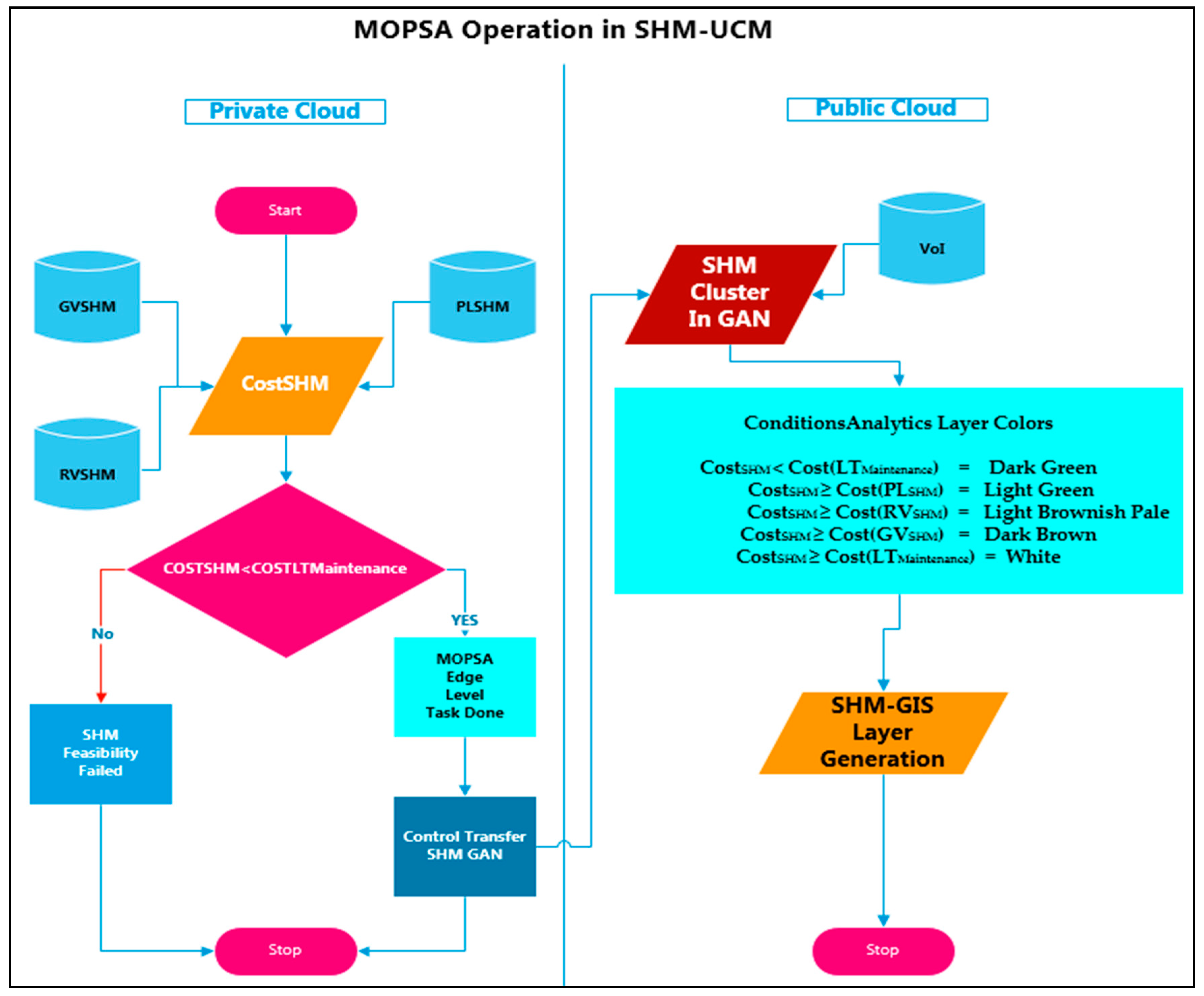
Section 4 discusses MOSPA, where the results are demonstrated in Section 5. MOSPA is a meta-heuristic sequential set of techniques that decides and evaluates the necessity of SHM in a geographical cluster under observation. The last section gives concluding thoughts and future recommendations about the proposed work.
The SHM-UCM has some limitations at software and hardware level. At the hardware level, all the sensors and networks defined in the architecture have to be homogenous with the structural variables needed. At the software side, the algorithm has to be incorporated with sequentially computed values from equations in a way that if some sensor value is missing it can approximate or interpolate from last two values in all fields to normalize the results. The results if not normalized will generate discrepancy between real time health on site and the one being shown on the layer generated by the SHM-UCM.
Moreover, GAN implementation limitation does exist as VSAT Data Packages prices provided by Satixfy [29], KiyuritsuRadio [30], Melat [31], and Telenor [32]. Price’s trends show an exponential decay in rates in coming years but right now out designed SHM-UCM GAN seems to only work on architectures like CubeSat and Thumbsat.

2. The SHM Utility Computing Model (SHM-UCM)

This work recommends a structured SHM that operates in compliance with a given Safety Integrity Level (SIL) and independently at Emergency Shutdown (ESD) level. SIL is governed by Structural Integrity Management (SIM) platform that over-rules decisions of Building Management Systems (BMSs). ESD is a binary decision based enveloped estimation that makes the structural health qualification criteria either passes or fail. SIM control parameters are set by GAN based on the geological, geographical, and geo-mechanic transients’ prediction assisted by weather stations. To this end, we present a SHM-GAN with heterogeneous Machine Learning (ML) algorithms engine in a distributed SIM framework at a lithosphere level, i.e., a separate SIM for a separate crust composition. Sandy, soiled, rocked, and limestone based areas have different foundation requirements for different type structures. GIS has critical databases of dynamic and real-time update in datasets for real patches on the crust.
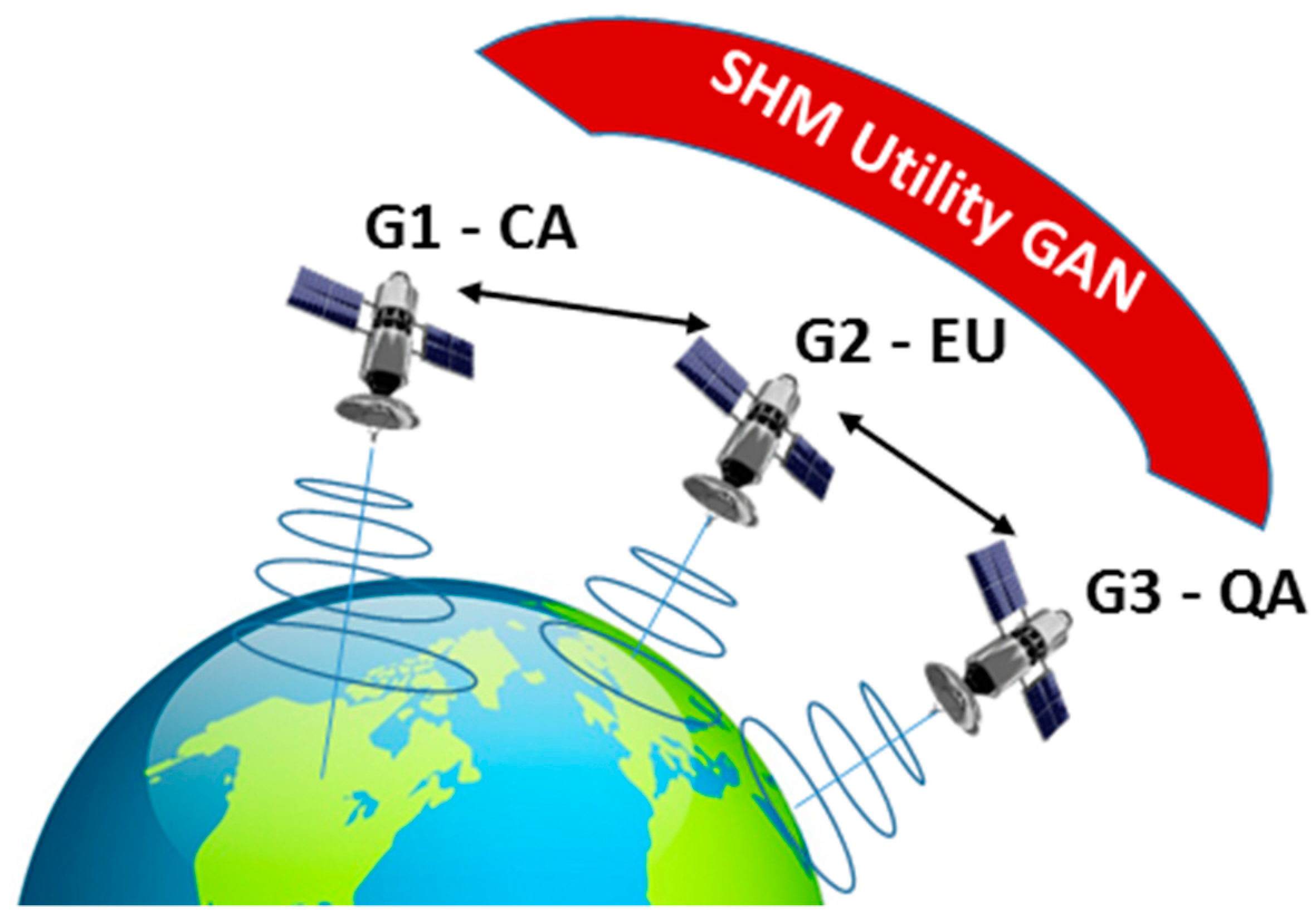
Figure 1 illustrates the proposed conceptual model of SHM-UCM networked through a mesh of SHM-GAN of the geospatial orientation of satellites dedicated for SHM. Three heterogeneous intracontinental patches are selected G1 for Canada, G2 for European Union and G3 for Qatar. Three different sizes have been selected to realize that freedom of observational geophysical patch selection. One each satellite i.e., G1, G2, and G3 decisions are made by MOSPA (proposed algorithm). This SHM-GAN enables globally engineered and administered implementation schemes for SHM for governments to reduce routine exhaustive calculations by Project Management Consultants (PMC). Quick tendering, systematic City, and Regional Planning (CRP) initiatives are examples of noticeable outcomes of this SHM-UCM, to mention few.
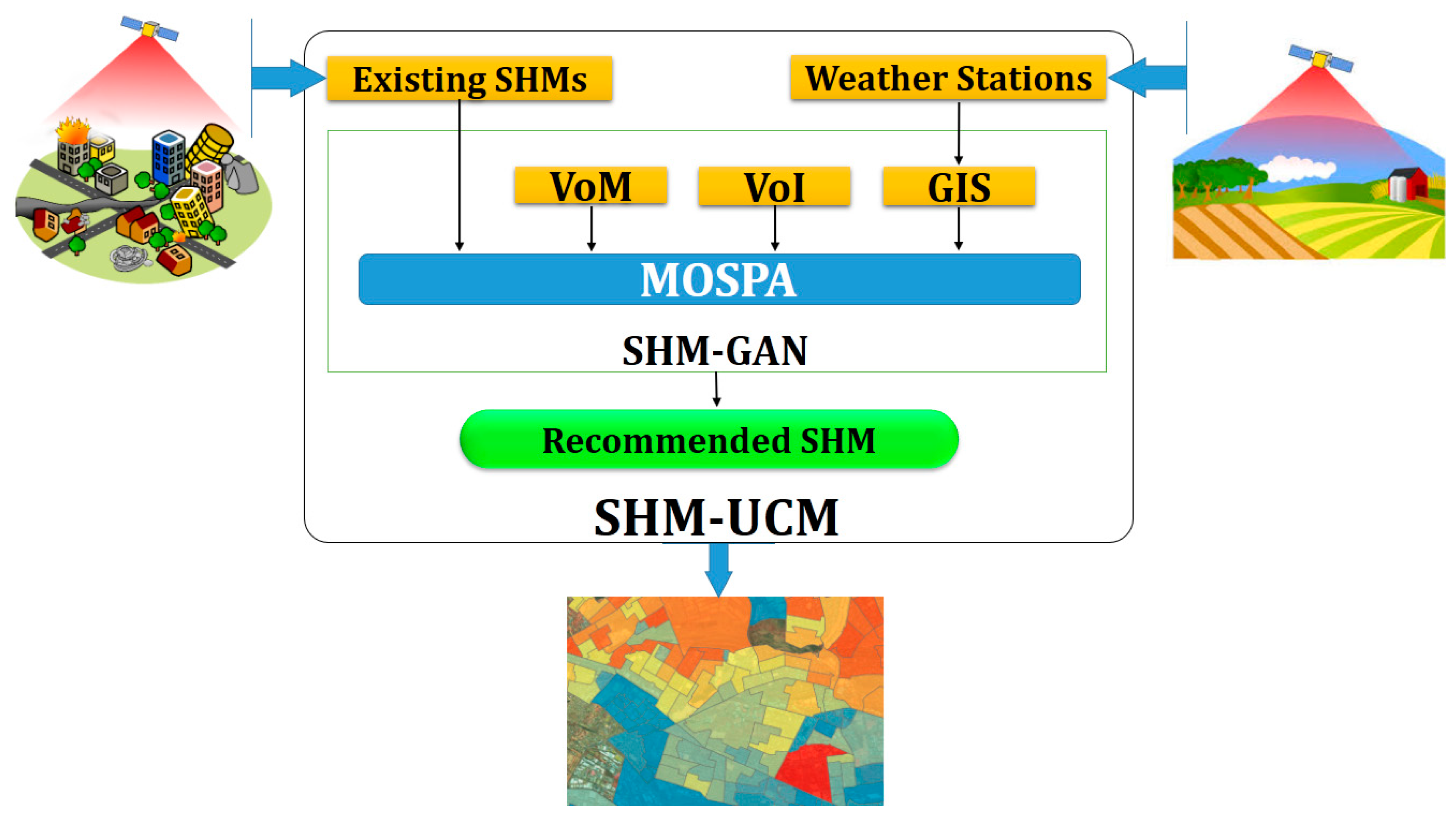
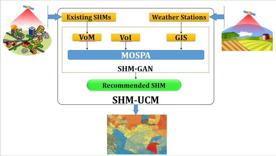
Figure 2 shows a complete overview of proposed SHM-UCM. It is evident that the data is taken from Existing SHM systems, Weather Stations GIS and VoI, analyzed by proposed MOSPA algorithm—resulting in SHM-GAN, i.e., satellite-based system running MOSPA. This complete analysis of input data and resulting in a geo plot for dynamically planning of SHM systems is ‘Structural Health Monitoring Utility Computing Model’. In real-time SHM systems for urban scale the need of private cloud is mandatory due to rapid response and for global scale the necessity of Public Cloud is mandatory. The private cloud has very fast response due to focused area and wide throughputs. On the other hand, the public cloud is dependent on worldwide internet is thus slower due to big bottlenecks, but has an advantage of IoT and GIS that a private cloud does not have.

3. Structural Health Monitoring Systems

The Body Area Heterogeneous Network (BAHN) for the SHM system is designed for a structure in which after hundreds of iterations in BIS frameworks, Value of Information is evaluated and finalized by multi-disciplinary Subject Matter Experts inputs to ML algorithm. A SHM is a sequential and systematic process in which the end product is a trustable abstract decision parameters dataset based on the data collected from SHM system variables. Firstly, the SHM is developed and deployed on structures-specific mandates that need to be monitored (e.g., residential, commercial, bridges, and tunnels). SHM system architecture is based on extracting upper and lower bounds of Finite Element Analysis (FEA) data. By upper and lower bound we mean the maximum and minimum values at which the structure is expected or meant to stay fully fit. A SHM system is a unique system that has to serve the purpose for lifecycle evaluation of structure for a structure for the next 10 years.
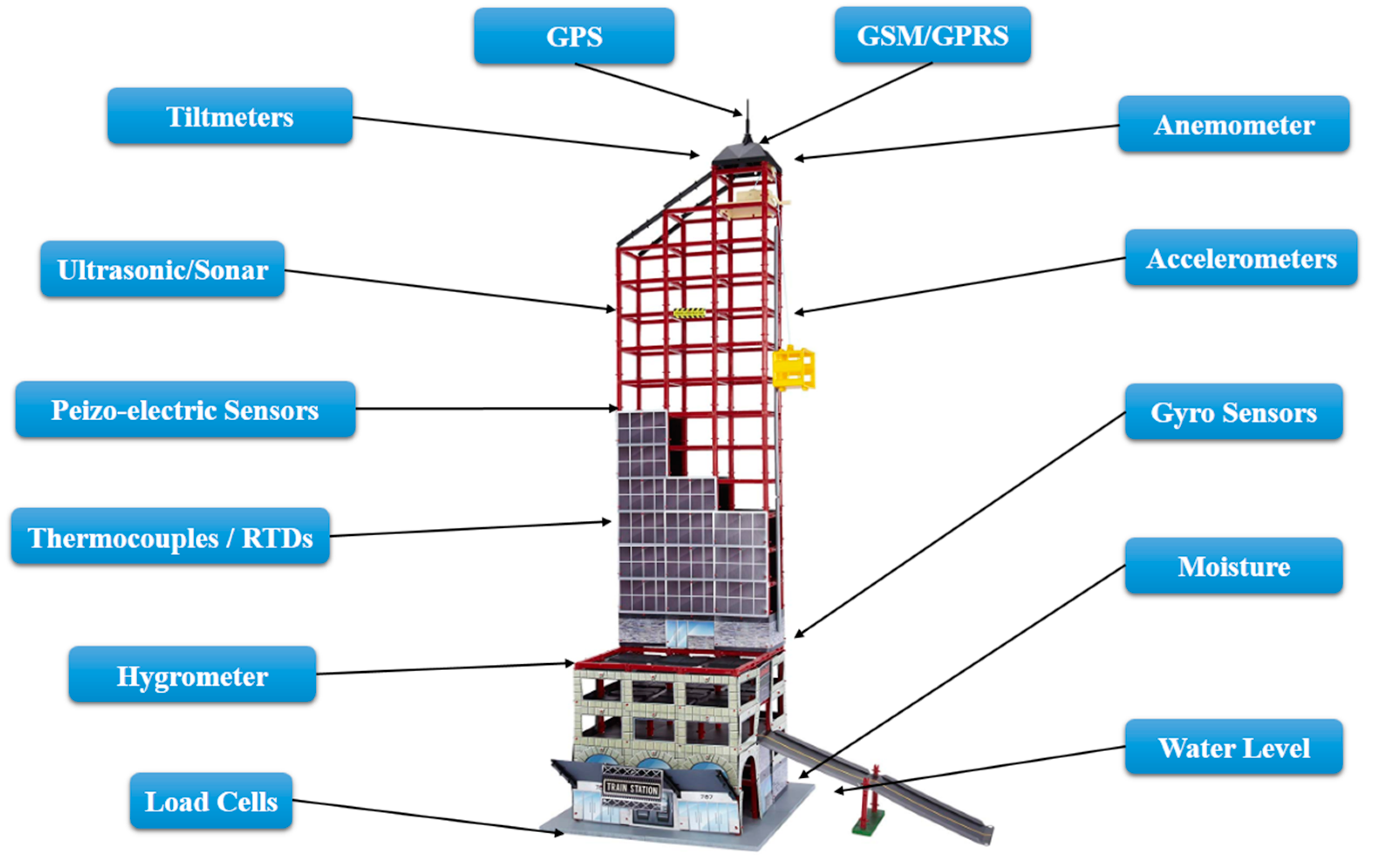
In Figure 3, a common SHM system has been shown based on Level of Detail 6 from building information system (BIS) documentation for a particular structure. This SHM system includes several sensors to measure the structure health, which includes weight (load cells), water level, moisture (hygrometer), balance (gyro sensors), temperature (thermocouples or resistance temperature detectors), accelerometers (vibration), pressure indoor and outdoor (piezo-electric sensors), collision or obstacle detection in vicinity (ultrasonic sensors or sonar), tilt and inclination (tiltmeter), and wind speed (anemometer). Secondly, the location and data communication is being achieved using GPS and GSM/GPRS, respectively. The variables shown vary from structure to structure and is a complex set of the formulation by a multi-disciplinary team. These variables can vary the SHM parameter estimation and feature extraction; in other words, directly affect the technical assessment of VoI of the respective structure. These SHM sensors have specific orientation and locations, which are calculated as per geospatial constraints. These sensors vary based on VoI calculated for the building and expected enormity of the disaster. This work is an effort toward the development of a smarter service oriented UCM that will bring the multi-disciplinary procedures and practices under one umbrella called SHM-UCM.
By 2018, the exponential rise in SHM nodes deployment has been registered across the world at institutional and organizational level with different topologies, architectures, and frameworks on various IoT platforms [17,
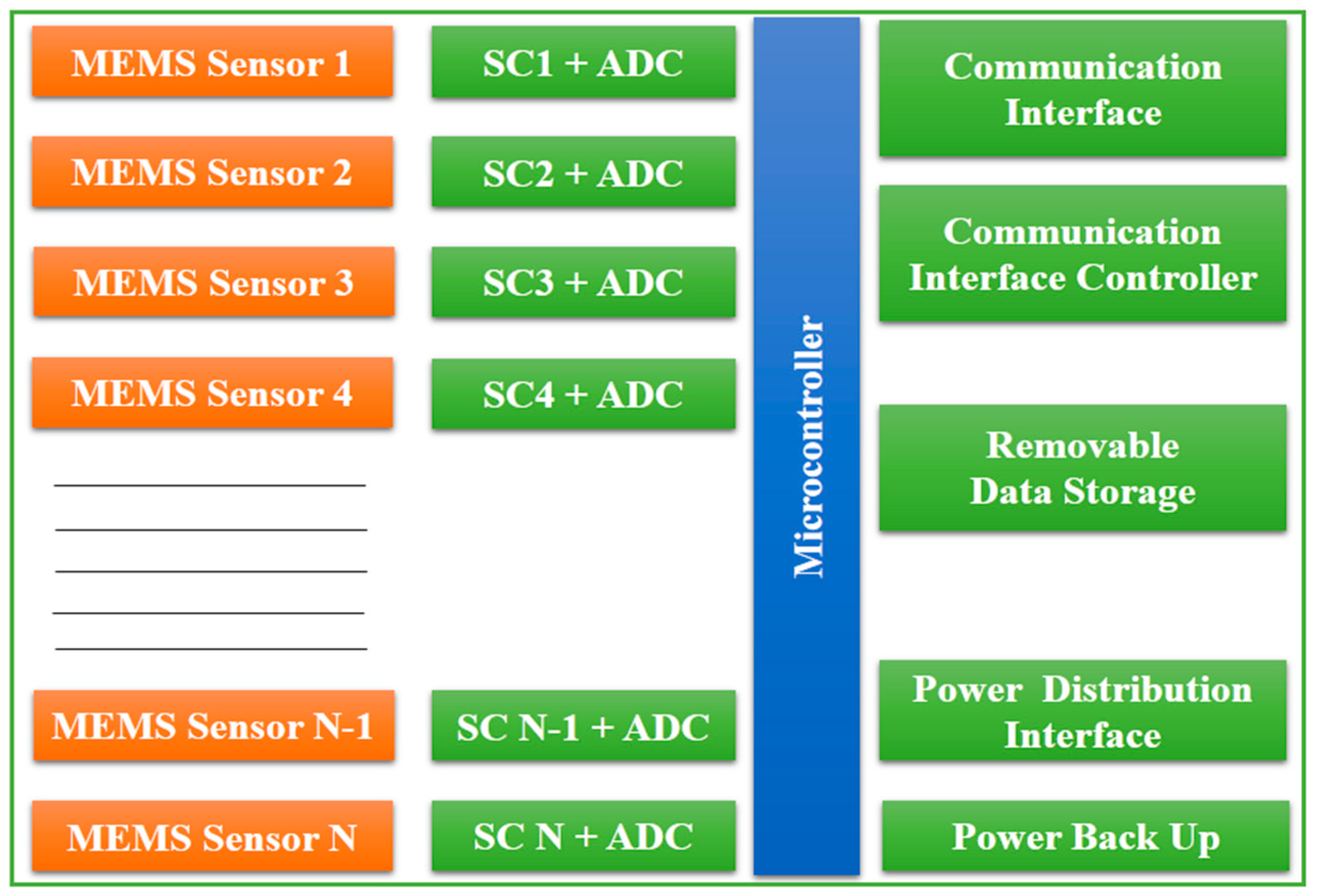
18]. For in-situ long-haul seamless monitoring, a most successful and frequent node architecture is used, which comprises a range of sensors, application specific scale Signal Conditioners (SCs), and high-resolution Analog to Digital Converter (ADC) chips and microcontrollers (e.g., Intel 8051, Microchip P18F458 and ATMega32).
Figure 4 illustrates a typical SHM node used for heterogeneous Body Area Network (BAN) implementations for existing SHM systems [19]. It has to go through a sequence of primitive data processing methods to be compatible with SHM systems. This SHM Node has to be orchestrated like a cloud framework ZeRo Client (ZRC), ThiN Client (TNC) and ThicK Client (TKC) nodes so that it fits in the ecosystem of Industry 4.0 standard for SHM systems.
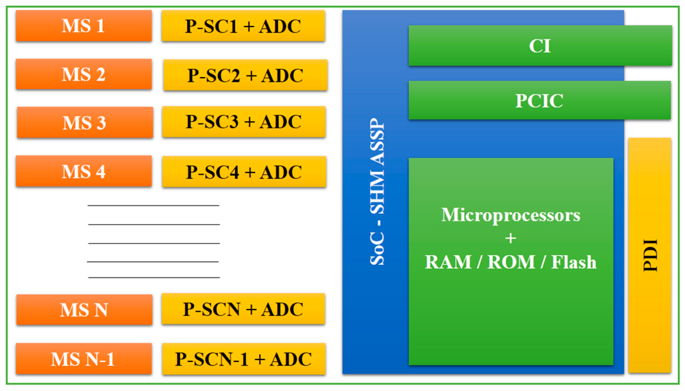
The SHM nodes proposed in this work are UCM coherent framework. The obligation of extreme sensitivity, scalability and sampling frequencies is imposed to achieve the variable data processing constraints for feature extraction techniques, Non-Destructive Testing (NDT) methods, and Non-Destructive Evaluation (NDE) procedures. It is repugnant to hire a new (different) team for detailed SHM parameter assessment every time. A SHM-Application Specific Standard Part (SHM-ASSP) fills the gap of providing the utility of high-resolution data for NDT and NDE assessment procedures.
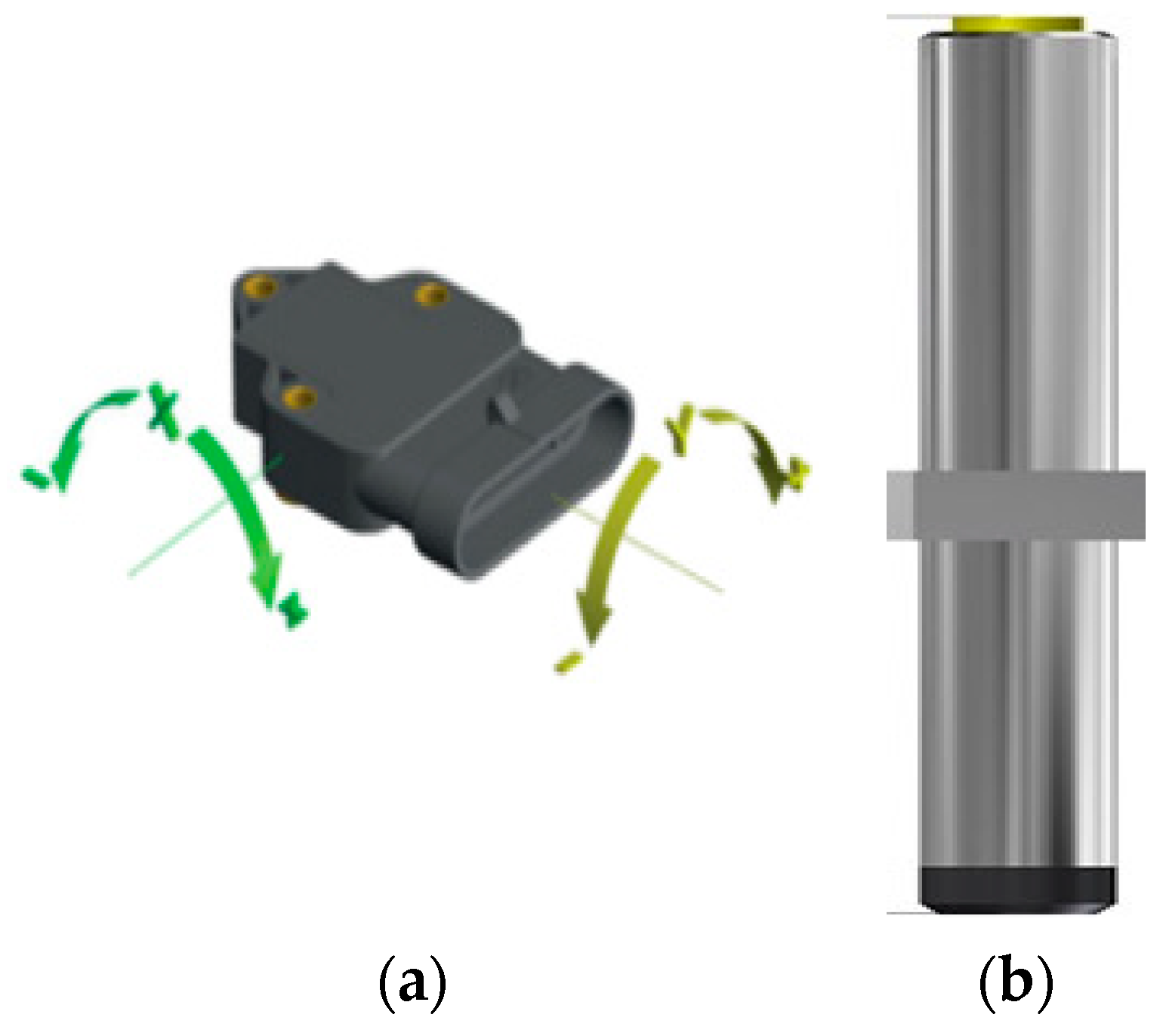
In Figure 5, a SHM-ASSP ZRC Node is illustrated that includes MEMS Sensors along with Programmable SC (PSC) to make it compatible with monitoring using specialized sensors and Programmable ADC (PADC) that can adopt scaling and range recommendation for particular observational criteria. The SHM-ASSP ZRC nodes proposed in this work need no external instrumentation assistance for SHM operations. ‘STM32F10RBT6’ CPU interfaced with inclinometers sensors are basic elements of nodes.
These nodes, which are developed in-house, are shown in Figure 6 and include:
  • Seismic Sensors Node with 2 SHM Sensors (SHM-ASSP ZRC-SSN)
  • Cylindrical Sensors Node full-fledged with 7 SHM Sensors (SHM-ASSP ZRC-CSN)
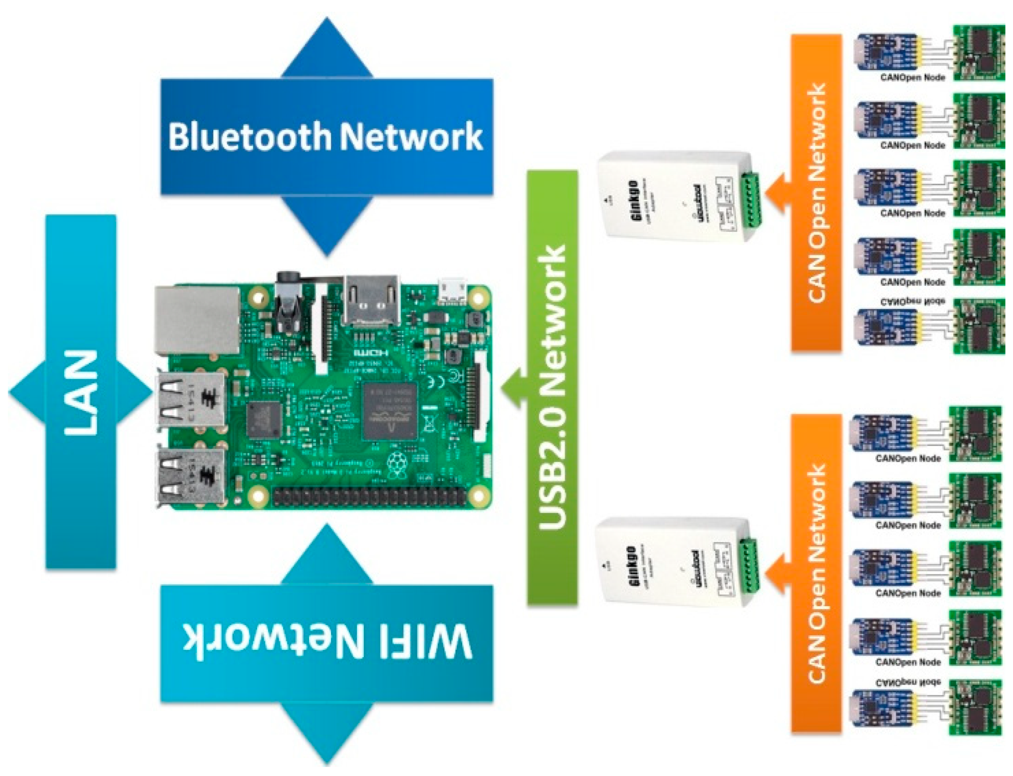
These nodes utilize CANopen industrial protocol paired with CAN-USB adapter to interface with an Out-Surface Board (OSB), in case of underground deployment, which transfers sensors readings wirelessly or wired to a gateway.
It is noteworthy to highlight that these nodes are enhanced with remotely programmable and configurable parameters.
Figure 7 shows an OSB that has a micro expert system with multiple resource-constrained Machine Learning SHM Algorithm.

4. Multi-Objective SHM Prediction Machine Learning Algorithm

SHM is highly feasible for bigger structures, especially community buildings, where structure value and human lives are critical. Multi-Objective SHM Prediction Machine Learning Algorithm (MOSPA) takes into account the results for SHM system parameters (i.e., Geometric, Real-time Sensing and Payload), then train an ML algorithm to give a geo plot for the dynamic planning of SHM. It uses a multi-objective Supervised ML Technique (SMLT), which streamlines the SHM Heterogeneous BAN architecture and steps of installation recommended by SHM-UCM.
The SHM is a synergy of multiple variables that can be static as well as dynamic. SHM parameters can be discretely illuminated as geometric or static parameters defined by the structural designer, sensed in real-time by capitalizing the instrumentation technology and the material strength of bearing the loads as the payload of a structure. SHM parameters can be generalized as three components for accurate health evaluation that are:
  • Geometric Variables (GVSHM)
  • Real-time Sensing Variables (RSVSHM)
  • Payload (PLSHM)
Figure 8 shows the big picture of MOSPA working model as its distributed operation at private and public level. MOSPA starts operation for initial or primary computations at IoT-edge level in SHM-OSB TNC. First assesses from cost conditions that SHM is feasible in the given structure or not if feasibility fails then disqualifies the structure for SHM installation. If cost condition is satisfies then starts sending data to of abstract cost computations shown in respective equations to GAN for more complex computations. In the public cloud, the VoI the architectural design level computations takes place with respect to parameters estimated in private cloud that have global effect and usability at urban and global scale infrastructure. The public cloud has multi-threaded servers for complex tasks.

4.1. Geometric Variables

The geometrical organs of a structure constitute its skeleton comprised of V o I B I M   that has all the definitions, i.e., floors   F B I M , beams   B B I M , columns   C B I M , joints   J B I M , trusses   T B I M , as defined by the structural architect. V o I B I M   is functional sum of functions of floors, beams, columns, joints, and trusses [22].
f ( V o I B I M ) =   f ( F B I M ) + f ( B B I M ) + f ( C B I M ) + f ( J B I M )   + f ( T B I M )
The structural parameters are measured or sensed using tiltmeters, accelerometers and ultrasonic sensor for offset measurement. The tilt in columns is measured using vertical angle θ y for columns, tilt in floors and beams is measured using horizontal angle θ x , the three dimensional vibrations or acceleration a x , a y , a z are deadlock for joints and trusses. Similarly, the distance or offset d x and d y between the parallel components like floor-to-floor and column-to-column is measured using ultrasonic sensors. All three variables for sure play their role in geometrical components. Let X and Y be the vital rectangular components for BIM components, i.e., a column, a truss, a beam, a joint, and a floor needs a 2D tiltmeter, 2D accelerometer, and 2D ultrasonic sensor. The time-series sum of the tilt, offset and acceleration should be equal to zero to justify that no deformation as occurred from time t 0 to t n in both axis X and   Y . Equation (1) can be written as a cost function of individual costs in X and   Y as:
C o s t ( f x ( V o I B I M ) ) = C o s t ( f x ( F B I M ) ) + C o s t ( f x ( B B I M ) ) + C o s t ( f x ( C B I M ) ) + C o s t ( f x ( J B I M ) ) + C o s t ( f x ( T B I M ) )  
C o s t ( f y ( V o I B I M ) ) = C o s t ( f y ( F B I M ) ) + C o s t ( f y ( B B I M ) ) + C o s t ( f y ( C B I M ) ) + C o s t ( f y ( J B I M ) ) + C o s t ( f y ( T B I M ) )  
It can be further elaborated as the sum of x and y components:
C o s t ( f ( V o I B I M ) ) =   C o s t ( f x ( V o I B I M ) ) + C o s t ( f y ( V o I B I M ) )  
For a 100% fit structure the sum of deformations should be equal to zero from time t 0 to t n in both axis X and Y and written as:
Δ C o s t ( f ( V o I B I M ) ) = Δ C o s t ( f x ( V o I B I M ) ) + Δ C o s t ( f y ( V o I B I M ) ) = 0  
The G V S H M cost fitness function is a condition when the sensed variables have zero difference from t 0 to t n
C o s t ( G V S H M ) = Δ C o s t ( f ( V o I B I M ) ) = 0  
C o s t ( G V S H M ) = C o s t ( t 0 t n X ( θ , a , d ) ) + C o s t ( t 0 t n Y ( θ , a , d ) ) = 0  

4.2. Real-Time Sensing Variables

The applied external variables parameter called R S V S H M computation depends on the temperature   T S H M , pressure   P S H M , wind effect   W S H M , the ground water level   L S H M , humidity   H S H M , and moisture   M S H M
f ( R S V S H M ) =   f ( T S H M ) + f ( P S H M ) + f ( W S H M ) + f ( L S H M ) + f ( H S H M ) + f ( M S H M )  
For an ideal structure that is 100% fit the costs of real-time variables should be equal to zero from time t 0 to t n
C o s t ( f ( R S V S H M ) ) =   C o s t ( f ( T S H M ) ) + C o s t ( f ( P S H M ) ) + C o s t ( f ( W S H M ) ) + C o s t ( f ( L S H M ) ) + C o s t ( f ( H S H M ) ) + C o s t ( f ( M S H M ) )  

4.3. Payload

The robustness of all structures depends on the material composition used for construction. Let the material stability constant be   M C M . The payload of a structure is a vital factor, that, if exceeded the rated limit defined by structural designer and transient behavior of material used, may damage the structure. Payload has is a dynamic variable and has two types: stationery S P L , and locomotive L P L . Stationery payload comprises of fixed material like tables, chairs, appliances, and all those things that stay at their place and cannot move at their own. Stationery payload can also be defined as a weight of non-construction material as w s . Locomotive payload is highly dynamic and transitional like humans and vehicles as weight w l . Payload is measured using load cells and occupancy models. Occupancy models are based on probabilistic approach. An instantaneous payload of a structure is the sum of the stationery and probabilistic locomotive payload and product of current material stability at a particular instance and is given as
f ( P L S H M )   =   f ( S P L ( w s ) ) +   f ( L P L ( w l ) )   ×   M C M
f ( L P L ( w l ) )   =   f   ( V o M )

4.3.1. User Identification from MAC and IMEI Addresses

A two-tier mechanism for occupant counters has been employed as occupant space called O v . O v is a sum of the number of MAC addresses registered in wireless routers (every PC or smart phone has a Wi-Fi card or a LAN card that has MAC address) plus IMEI that every smart phone has as a de facto de jure for Electronic Industry Association/Telecommunication Industry Association approved the standards. These two variables overlap, but gives a complete overview of all the electronic devices in a particular location; mobile phones with SIM card and devices connected to Wi-Fi.
O v   =   Σ ( M A C )   +   Σ ( I M E I )

4.3.2. Attendance Count

For permanent inhabitants or occupants’ biometric access counter, I is defined in terms of O p as:
O p   =   Σ I
Thus O is summed up as
O   =   O v   +   O p
The total occupancy probability distribution function is taken to obtain a random occupancy vector at a specific location.

4.3.3. Final Population Count

In a given model [20,21], hourly Probability Distribution Functions (PDFs) that allow the calculation of the probability for a particular occupancy state occurring within a given hour is presented. Let H   =   ( O 1   O m )   denotes all occupancies that occur per second during a period of time and V x is a vector of occupancies for room x , where x =   1 , 2 ,   3 ,   .   y . Let α i denote the average occupancy for the room r i . We calculate a vector of means α   =   ( α 1 ,   ,   α m ) and covariance matrix M from O . Using α and M , we define a Probability Density Function f :
f ( V o M ) = 1 1 ( 2 π ) n 2     | M | 1 / 2 exp { ( O α ) T M 1 ( O   α ) 2 }
Hourly Gaussian models with mean α h   and covariance matrix M h , where f can give a probability of an occupancy occurring for a specific dataset O h for hour   h , is defined. Using this function, random occupancy vectors can be drawn from the distribution.
The final population count is obtained by removing the overlaps between the MAC, IMEI addresses and attendance count. A condition is applied that if the MAC, IMEI addresses are at a close distance to a person counted for attendance, all should be counted as one person. Similarly, if registered MAC s and IMEI addresses are at less than half a meter, it should be considered as a single person, i.e., that person has a cell phone with IMEI address and a laptop with MAC address connected to Wi-Fi, but he or she has not put the attendance through biometric access count. Then after calculating the final population count at a specific time step, a PDF can be obtained.
Equation (16), i.e., fitness function should have zero cost from time t 0 to t n to be 100% fit in ideal case is change in the sum of stationery and locomotive cost and change in material stability cost and is written as:
Δ C o s t ( f ( P L S H M ) )   =   Δ C o s t ( f ( S P L ( w s ) ) +   f ( V o M )   ×   M C M )   =   0
The final output of our MOSPA is a final cost function as value that will define the fitness of structures leading to qualification of a geospatial patch under observation. From Equations (7), (9), (10), and (16) for respective quantifications SHM-UCM layer equation can be written as lifetime predicted maintenance cost of a structure as Cost(LTMaintenace) for expected utility factor, as described in [33] Equation (32), and is given as:
Cost(LTMaintenance) = Cost (GVSHM) + Cost(RVSHM) + Cost(PLSHM)
Ideally the Cost(LTMaintenance) of a structure should be greater than the cost of SHM (CostSHM) installed in the structure. Practically it has slight variations like a difference of ±10%. If the SHM cost exceeds the lifetime cost at any point it is termed as a failed installation.
CostSHM ≤ Cost(LTMaintenance)
Furthermore, the layer generation aspect is computed using change in lifecycle cost or structure and is defined in the form of Table 1 given below
In Table 1, the worst color is White means SHM is not installable or extremely costly.

5. Case Study: SHM Systems in Qatar University

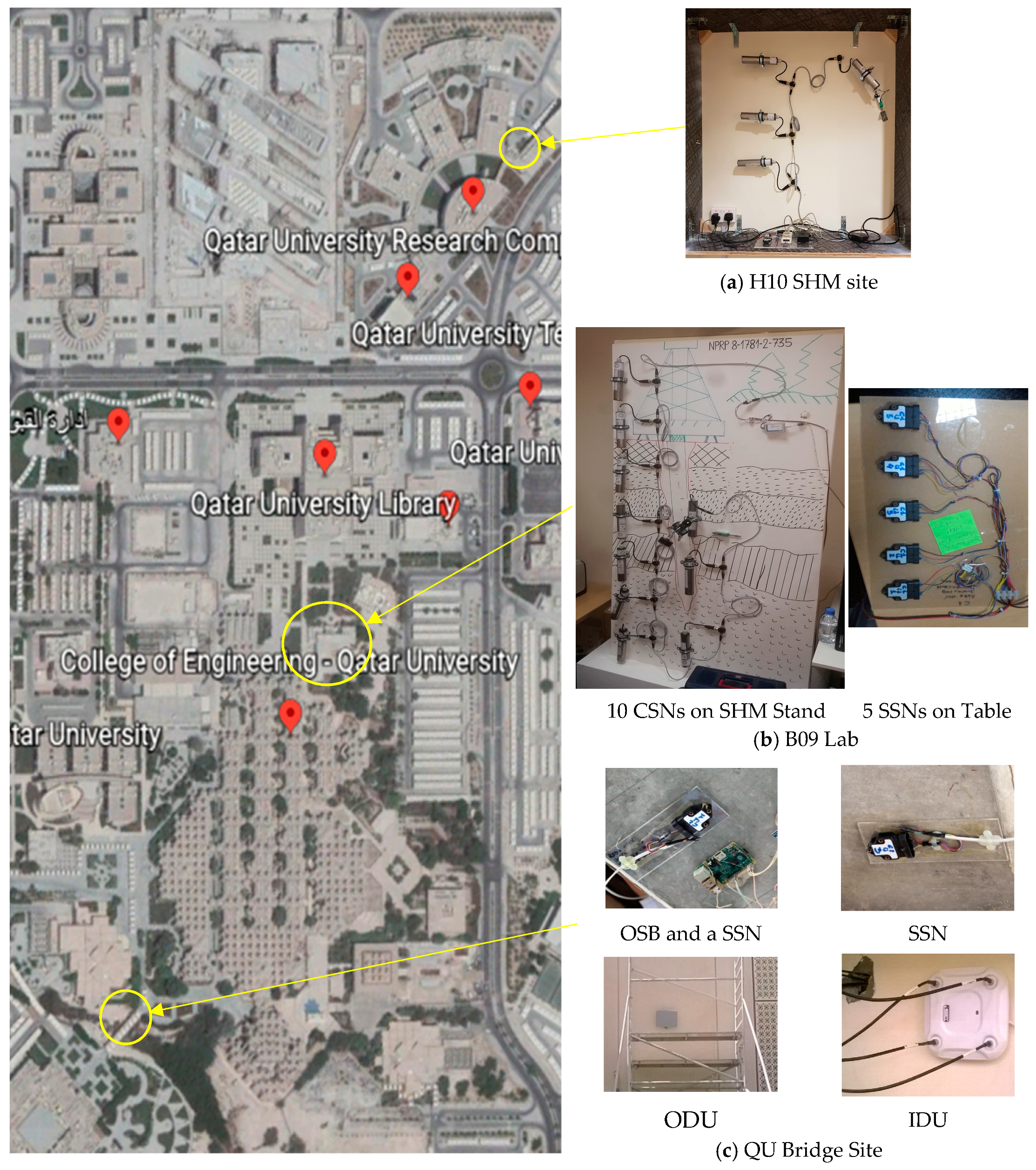
The chosen case study is SHM system prediction for Qatar University (QU) from GAN based SHM-UCM. Three different specification and configuration systems were installed in QU at three 1 km apart unique locations, namely, B09 Lab, QU Bridge and Research Complex H10 with geometric variables monitoring capabilities for 6 months. The QU Bridge has maximum human movement (pedestrians and vehicles), the H10 has construction sites in its vicinity thus incurring various vibrations, and B09 Lab is our benchmarking or standard facility where we have SHM Test bench having eight nodes. The SHM system details for these locations are:
  • QU bridge SHM Site (SHM-BS) System with 4 SHM-ASSP-ZRC-nodes.
  • H10 SHM site (SHM-RC) with 4 SHM-ASSP-ZRC-SSNs
  • B09 Lab site (SHM-LB) with 4 SHM-ASSP ZRC-SSNs and 10 SHM-ASSP-ZRC-CSNs
The entire deployment plan for case study QU is shown in Figure 9, published in our earlier papers was uploading data to Thingspeak IoT platform by Mathworks. Raspberry Pi 3 is being used as an out-surface board (OSB), i.e., SHM-UCM-TNC. All CSNs and SSNs are SHM-UCM-ZRCs nodes. The 2 km+ WiFi range extenders from CISCO are indoor data unit (IDU) and outdoor data unit (ODU). This system encompasses practical limitations that would be inherently considered in our UCM.
Common problems that are generally faced in generic/conventional SHM deployments, and are overcome in this work are:
  • For every site, one has to click on the IoT links to explore, which is not feasible in urban scale solutions in cases where we might have 10,000+ buildings.
  • The 15 s lag in every variable on ThingSpeak is a real hurdle in real-time geo-analytics.
  • No real-time algorithm with data processing capabilities above 100 MB/s should be used in public cloud based solutions, as well as urban scale geo-informatics applications.
  • Even an organizational level SHM is impossible in existing scenario, i.e., totally impossible at urban scale where there are more than 200 organizations.
  • An application specific web-based private cloud SHM platform with the geo-analytics capabilities has so far been absent.
  • An algorithmic scalable sensor based GIS layer generation mechanism has so far been missing.
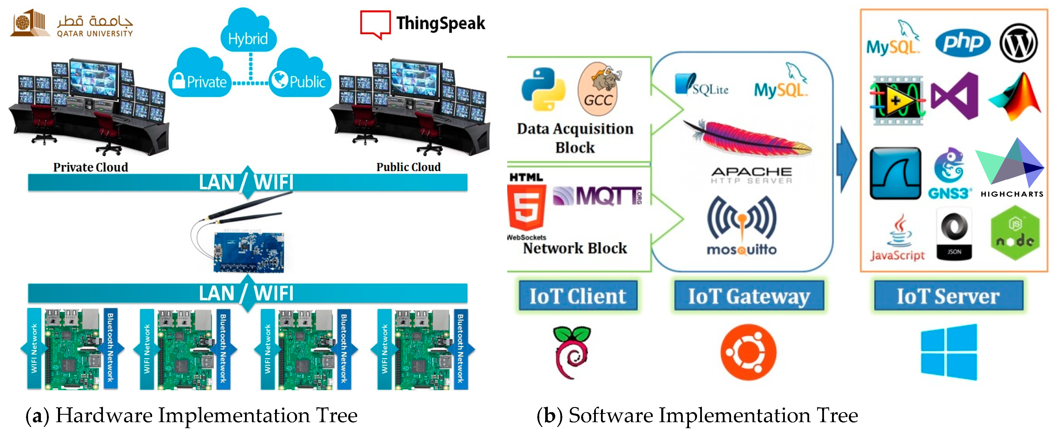
A comprehensive software and hardware architecture to implement the SHM-UCM is given in Figure 10. In Figure 10a, there are four Raspberry Pis (OSB) and Banana Pi R1 gateway serving as SHM-UCM-TNCs. Dell PowerEdge 28XX Series Rack Servers are used SHM-UCM Servers. In Figure 10b, OSBs are the IoT clients, Banana Pi R1 is the IoT gateway and Dell PowerEdge Servers are having the LAMP Server.

6. Results and Discussion

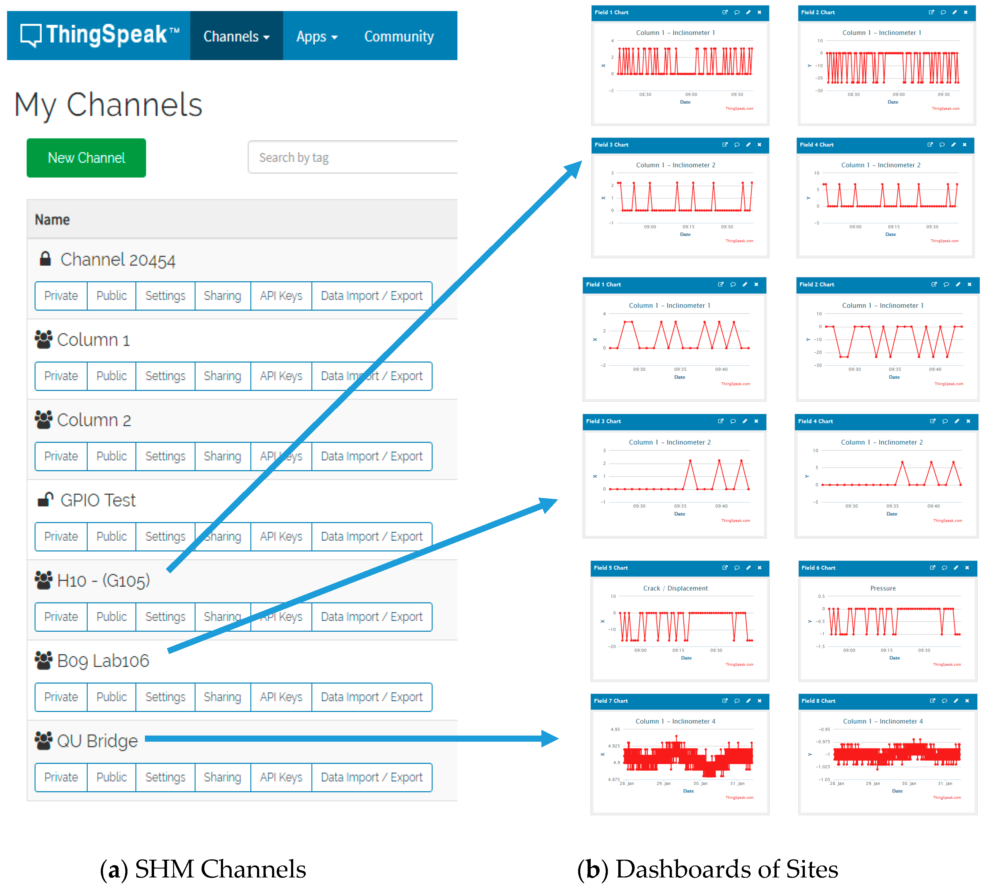
Three sites are pooling data to ThingSpeaks IoT platform with the problems mentioned in thecase study and that are being displayed in the figures below. In this work, the geometric nodes data was used i.e., θ , a , d . The B09-Lab test bench is sending to data to LabView just for comparison as well as the ThingSpeak IoT and private cloud SHM-UCM Server with MOSPA. The QU Bridge and H10 sites sending data to ThingSpeak and well as private cloud SHM-UCM Server with MOSPA. This work was using 80,000 samples from three sites, as mentioned, but now all the processing is live and highly data efficient and robust. Below are shown the ThingSpeak IoT plots that are just for reference.
Figure 11 shows that all sites are working fine and pooling data immaculately. The challenge for MOSPA is the low data rate (i.e., 15 s) for single variable update, which is visible from Figure 11b. This is being highlighted in Thingspeak reference manual. This work uses JSON published over the SHM-UCM and stored as a DB file at the server. The above results show that real-time geo-analytics is slow when using the Thinkgspeak platform.
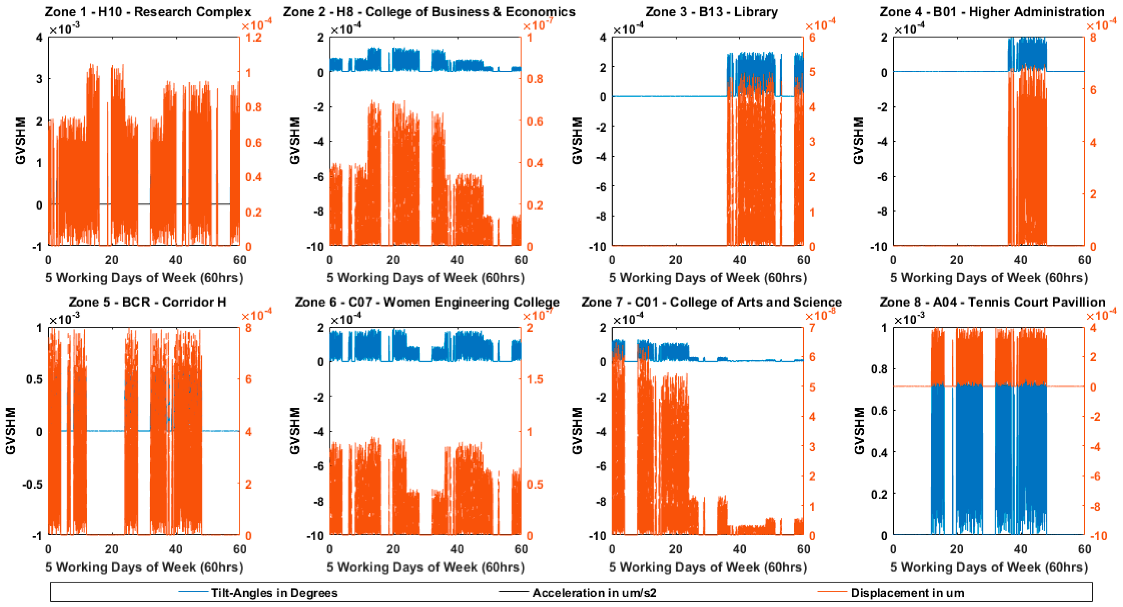
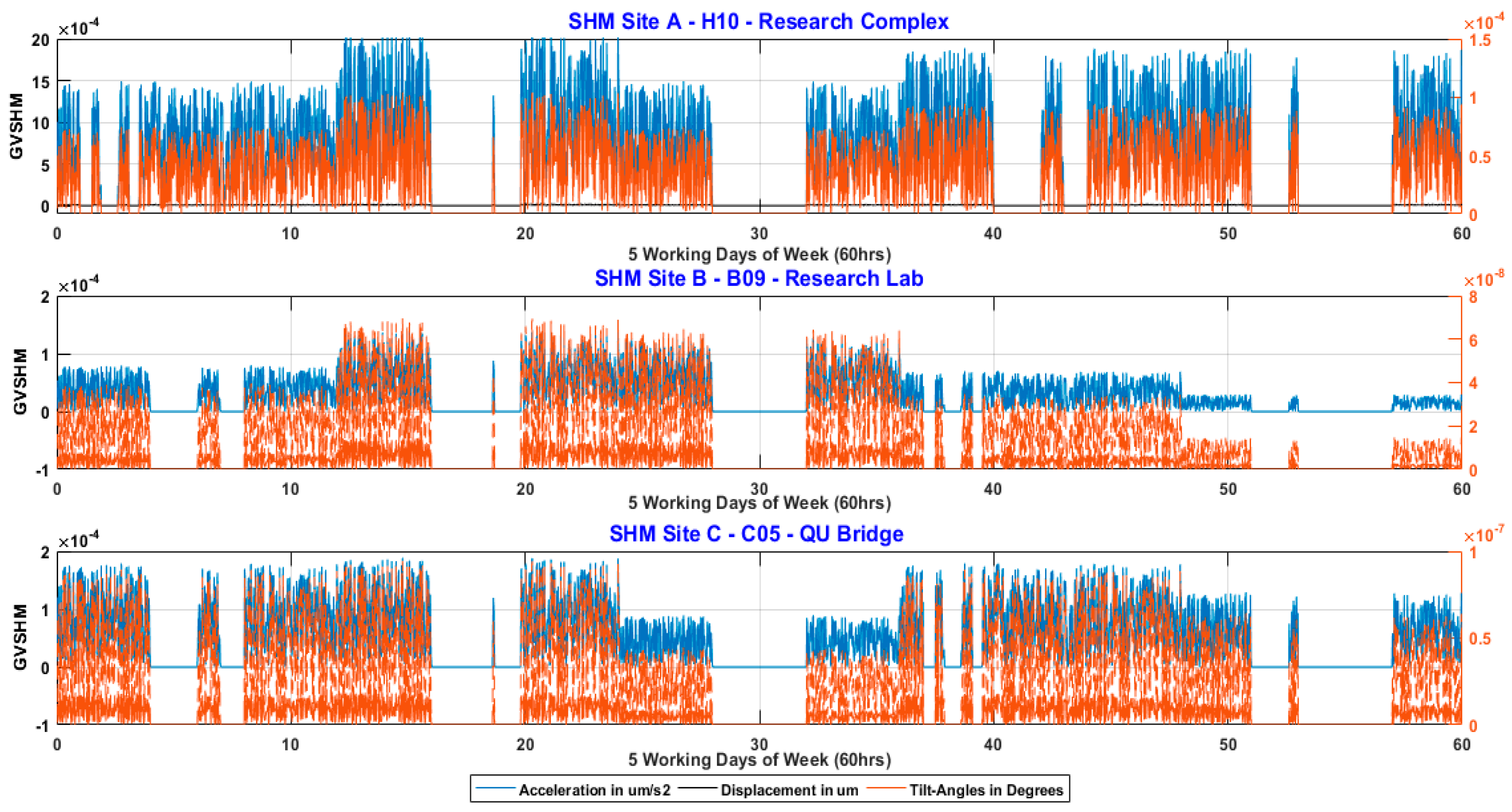
We did the same experiment and collected data using our private Cloud platform. The results are shown in Figure 12, in which the GVSHM plot of tilt angles, accelerometers and displacement sensors are visible with a constant trend of acceleration and displacement overlapping each other. This would indicate that the structures are extremely safe. The results of MOSPA are sequential in nature. First computation is runtime geometrical variables time-series trend. The DB data for three sites shows as stationarity in nature.
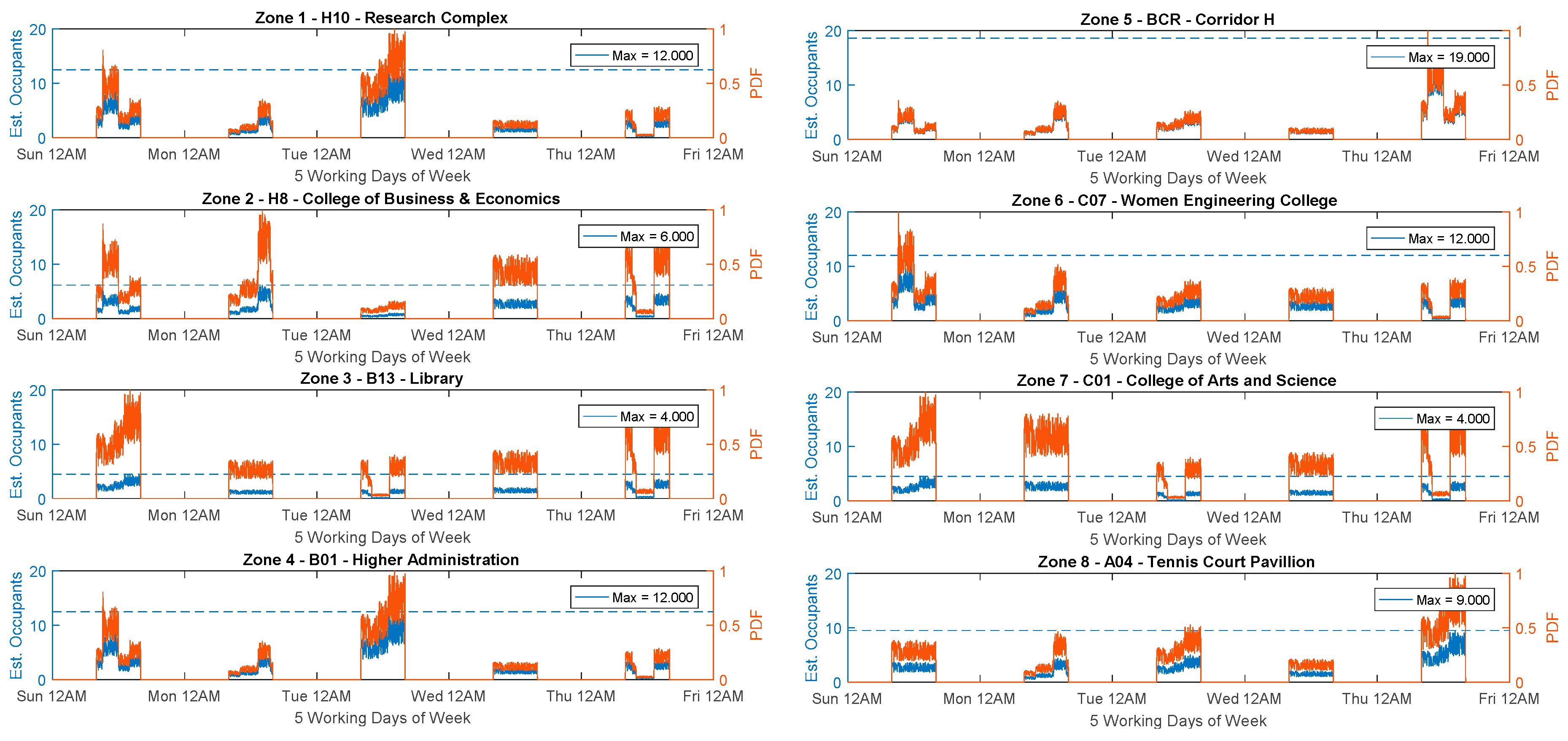
By using actual occupancy that is based on daily attendance and vibrations measured by SHM three sites, MOSPA created eight zones based on occupancy. The Variable Occupancy Model (VoM) map is based on the probability density function of occupancy O given in Equation (4). The PDF in (4) forecasted the occupancy by adopting the historical data of O , α , and M , as discussed before.
Figure 13 shows the simulation results obtained from the PDF in Equation (4) by GAN selected zones based on the estimated number of occupants per week (five working days). The blue line is the actual number of occupants present sensed from MAC addresses of PCs and smart phones and red line shows the predicted or expected occupants. The number of occupants must not exceed the rated payload, i.e., 50% of rated payload for a building in any zone. The results show that maximum occupancy was observed in Zone 5: BCR Corridor H (19 persons), Zone 1: H10 Research Complex (12 persons) Zone 4: B01 (12 persons), and Zone 6: C07 (12 persons).
In Figure 14, MOSPA utilized the 8 zones created using the real attendance and predicted attendance to generate the expected 8 zones recommended for GVSHM, RSVSHM and PLSHM. variables where the installation of SHM can improve the safety of occupants given in Figure 15.
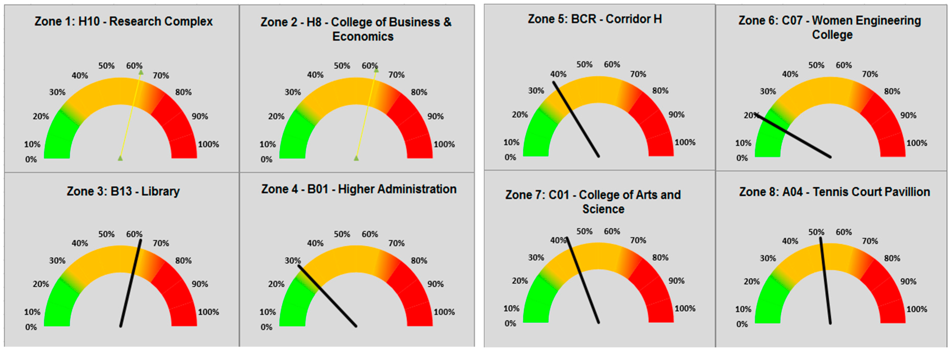
Figure 15 shows cumulative fitness percentage of occupancy in structures from Zone 1 to 8 obtained by the estimated SHM system results (from Figure 16). Two colors of needles are visible in 
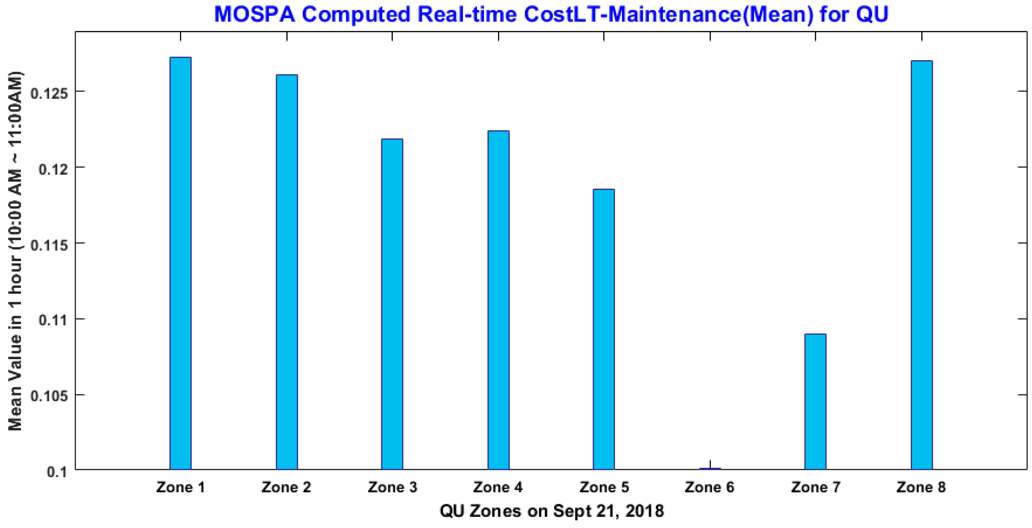
Figure 16, where the golden ones show maximum overshoots or SHM with maximum utilization of structure, whereas the black ones show that below 50% of sensors in SHM have almost constant values. The plots in Figure 18 for predicted cost are very realistic since indeed both H10 and H08 has a maximum flow of occupants that should result in maximum vibration, the maximum change in pressure, humidity, and temperature.
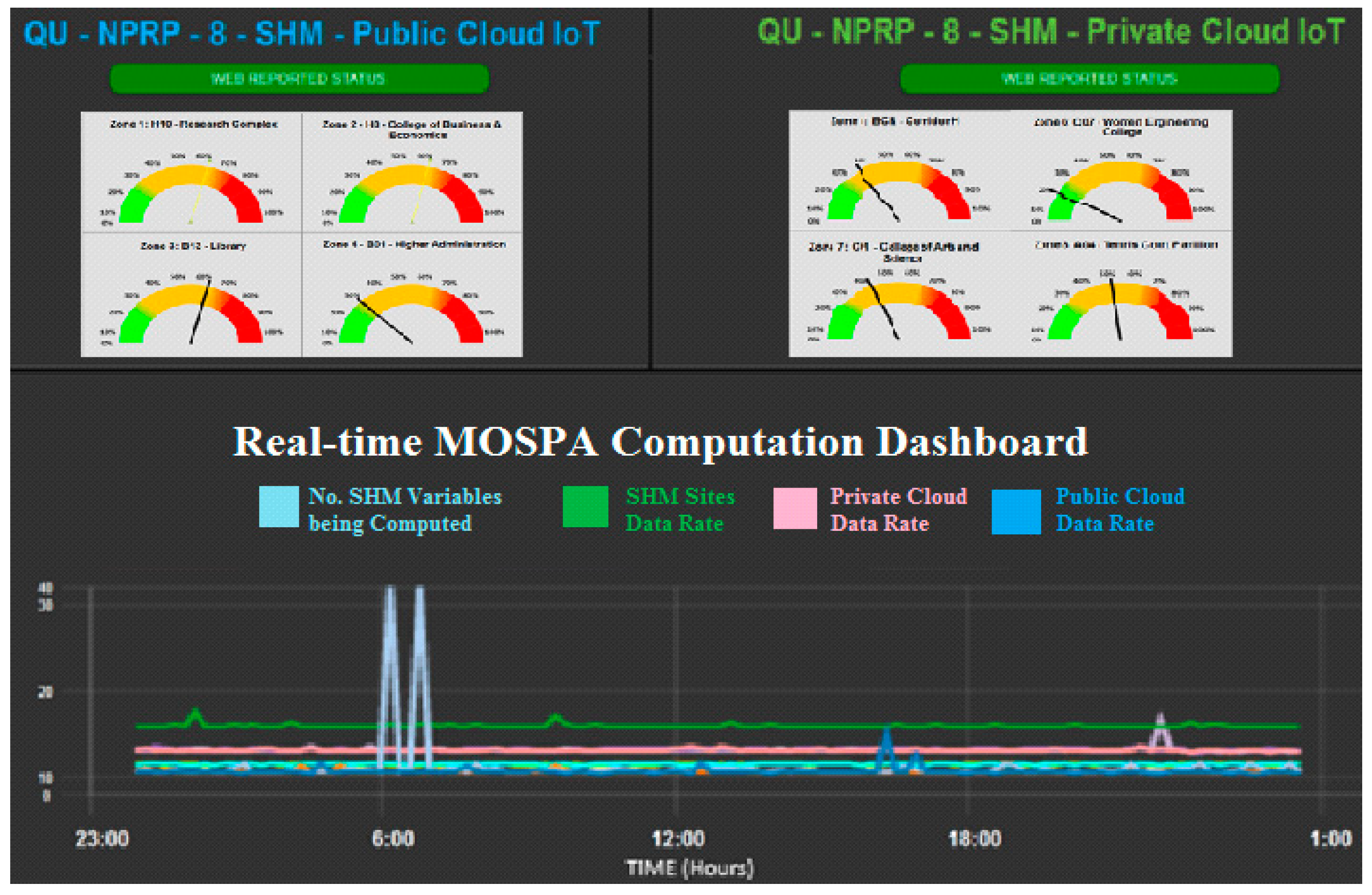
The overall dashboard with noticeable suitability for SHM-UCM in urban scale applications can be observed in Figure 16. For urban scale geo-analytics the constraint for abstract results is important. One can access the details for further investigation in utility computing cloud for troubleshooting and systems detailing purposes. In Figure 17, desired goal achieved for an urban scale SHM based geo-informative system can be seen from line plot that bottlenecks have been reduced by only transmitting the abstract computation to the public cloud for optimized GAN traffic payloads.
In Figure 17, the output of Equation (17) is displayed, as computed on 21 September 2018. This data is a paramount metric for building management to study and act if needs be. The range of cost is between magnitude zero and one. The magnitude zero means no maintenance is required and the structure is adequately fit. The magnitude one means totally damaged structure, i.e., unrepairable. The zero value will be displayed as ambient green and one will be ambient brown or dust-colored in geo-plot at urban scale GIS layer below.
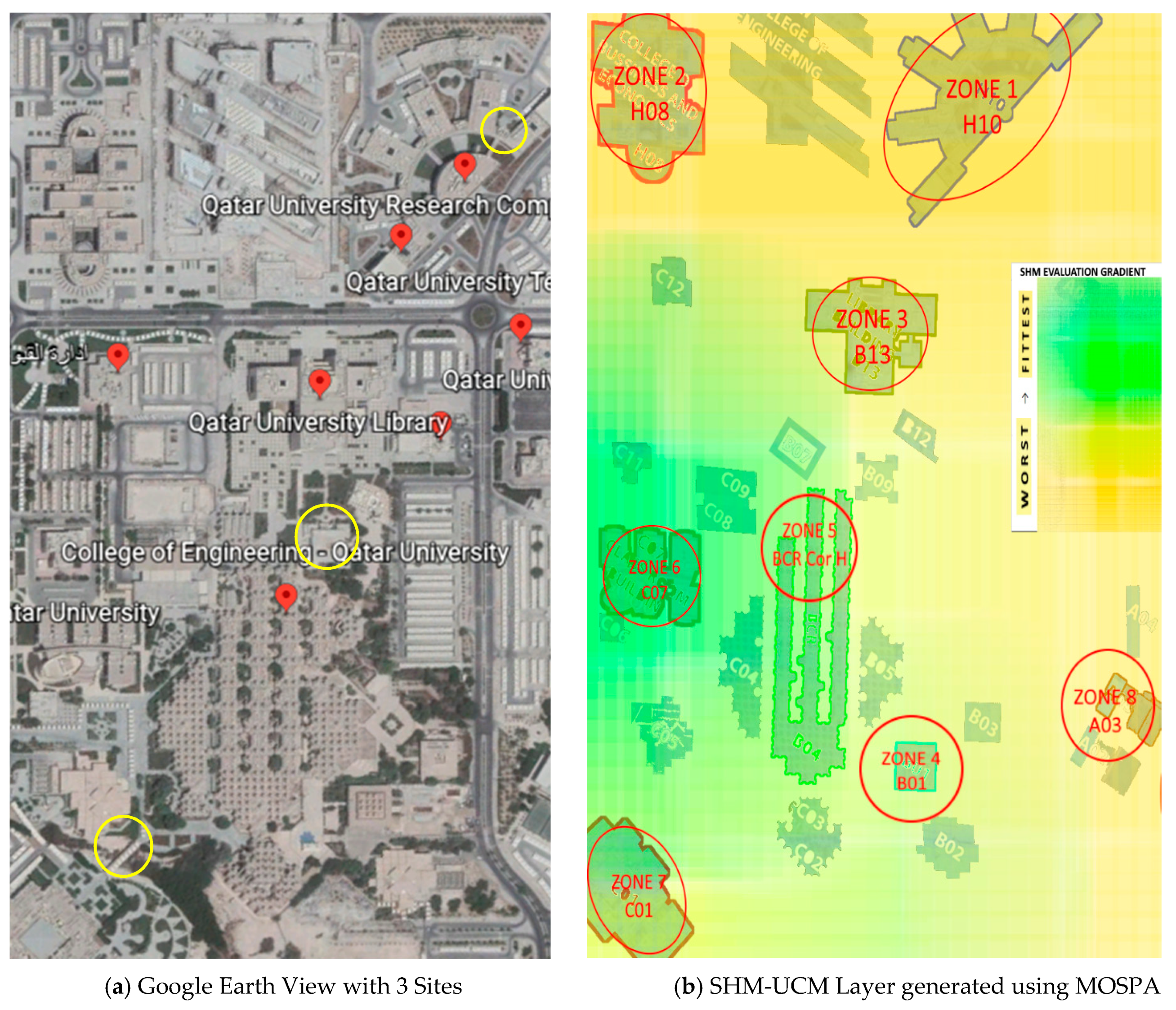
In Figure 18, the final output geo-plot is presented in a visual yet user-friendly interface as a result from an automated decision-making map for helping building management. The interpolation of magnitudes from Figure 18 has assisted in the generation of SHM-UCM GAN plot by MOSPA or SHM-UCM GIS layer for QU geo-spatial patch.
Figure 18 shows the resulting MOSPA geo-plot that can be used for dynamic re-planning of SHM. The dark yellow reading presents unfit conditions for structure health, whereas the dark green indicates the fittest building (refer to Figure 9 for comparison). The unfit condition can be due to several reasons such as critical historical building status or higher occupancy. The proposed SHM-UCM model, working over the GAN satellite-based system, can be utilized as a tool for an in-depth survey of geographical areas, as well as disaster management.

7. Conclusions

A SHM-UCM on GANs for real-time decision making for a geospatial cluster has been proposed. Decision-making is made possible by a novel MOSPA model that processes variables from heterogeneous patches. We found that (i) greater variety of sensors has led to better SHM and cost estimation and condition of structures, (ii) the application of geographical, local (in-situ) variables along with a payload of system can lead to very precise and trustable results, and (iii) in urban scale geo-informatics applications are mandatory to have abstract results for decision making on the go instead of lower and deeper details. An abstract SHM layer concept for GIS and SHM-UCM introduced in this work is a novel contribution that is quite instrumental for urban planning industry. A case study was conducted on Qatar University buildings to test the proposed algorithm. The results presented are an approximation of real-time analysis of structures health, which has identified critical cases where more SHM nodes are required to efficiently measure structural health for improved early warnings. While this study did not take an engineering approach to characterizing structural health dynamics, the monitoring platform integrating GIS and UCM presents an urban-scale decision-making tool in form an SHM-UCM that would help organizations in framing precise disaster management policies and infrastructure planning by multi-objective computation support using MOSPA. We propose that the tender, proposal document, and contractual agreements must include SHM-UCM and modern risk mitigation techniques.

Author Contributions

Conceptualization, Hasan Tariq and Anas Tahir; Data curation, Hasan Tariq and Anas Tahir; Formal analysis, Hasan Tariq and Anas Tahir; Funding acquisition, Farid Touati, Mohammed Abdulla E. Al-Hitmi, Damiano Crescini and Adel Ben Manouer; Investigation, Hasan Tariq and Anas Tahir; Methodology, Hasan Tariq and Anas Tahir; Project administration, Farid Touati; Resources, Farid Touati, Mohammed Abdulla E. Al-Hitmi, Damiano Crescini and Adel Ben Manouer; Software, Hasan Tariq and Anas Tahir; Supervision, Farid Touati; Validation, Hasan Tariq and Anas Tahir; Visualization, Hasan Tariq and Anas Tahir; Writing—original draft, Hasan Tariq; Writing—review & editing, Anas Tahir, Farid Touati, Mohammed Abdulla E. Al-Hitmi, Damiano Crescini and Adel Ben Manouer.

Funding

This publication was made possible by NPRP grant # 8-1781-2-725 from the Qatar National Research Fund (a member of Qatar Foundation). The publication of this article was funded by the Qatar National Library. The statements made herein are solely the responsibility of the authors.

Conflicts of Interest

The authors declare no conflict of interest. The funders had no role in the design of the study; in the collection, analyses, or interpretation of data; in the writing of the manuscript, or in the decision to publish the results.

References

  1. Farid, T.; Hasan, T.; Adel, B.M.; Damiano, C. Design and Simulation of a Green Bi-Variable Mono-Parametric SHM Node and Early Seismic Warning Algorithm for Wave Identification and Scattering. In Proceedings of the 14th International Wireless Communications & Mobile Computing Conference (IWCMC), Limassol, Cyprus, 25–29 June 2018. [Google Scholar] [CrossRef]
  2. Agdas, D.; Rice, J.; Martinez, J.; Lasa, I. Comparison of Visual Inspection and Structural-Health Monitoring As Bridge Condition Assessment Methods. J. Perform. Constr. Facil. 2016, 30, 04015049. [Google Scholar] [CrossRef]
  3. Engel, A.; Liebig, B.; Koch, A. Energy-Efficient Heterogeneous Reconfigurable Sensor Node for Distributed Structural Health Monitoring. In Proceedings of the 2012 Conference on Design and Architectures for Signal and Image Processing, Karlsruhe, Germany, 23–25 October 2012. [Google Scholar]
  4. Dong, X.; Chen, S.; Zhu, D.; Kane, M.; Wang, Y.; Lynch, J.P. High-Speed Heterogeneous Data Acquisition using Martlet—A Next-Generation Wireless Sensing Node. Structure 2014, 8, 9. [Google Scholar]
  5. Kijewski-Correa, T.; Haenggi, M.; Antsaklis, P. Wireless Sensor Networks for Structural Health Monitoring: A Multi-Scale Approach. In Proceedings of the Structures Congress 2006: 17th Analysis and Computation Specialty Conference, St. Louis, MO, USA, 18–21 May 2006. [Google Scholar]
  6. Ozer, E. Monitoring Bridge Vibrations via Pedestrians and Mobile Sensing. In Proceeding of NDT Canada 2018, Halifax, NS, Canada, 19–21 June 2018. [Google Scholar]
  7. Kotsakos, D.; Sakkos, P.; Kalogeraki, V.; Gunopulos, D. SmartMonitor: Using Smart Devices to Perform Structural Health Monitoring. Proc. Vldb Endow. 2013, 6, 1282–1285. [Google Scholar] [CrossRef]
  8. Jang, M.; Lee, H.; Bhardwaj, K.; Schwan, K. vSensor: Toward Sensor-rich Mobile Applications; Georgia Institute of Technology: Atlanta, GA, USA, 2014. [Google Scholar]
  9. Jang, M.; Lee, H.; Schwan, K.; Bhardwaj, K. SOUL: An Edge-cloud System for Mobile Applications in a Sensor-rich World. In Proceedings of the 2016 IEEE/ACM Symposium on Edge Computing, Washington, DC, USA, 27–28 October 2016. [Google Scholar]
  10. Zaki, G.; Plishker, W.; Li, W.; Lee, J.; Quon, H.; Wong, J.; Shekhar, R. The Utility of Cloud Computing in Analyzing GPU-Accelerated Deformable Image Registration of CT and CBCT Images in Head and Neck Cancer Radiation Therapy. IEEE J. Transl. Eng. Health Med. 2016, 4, 1–11. [Google Scholar] [CrossRef]
  11. Yu, R.; Ding, J.; Maharjan, S.; Gjessing, S.; Zhang, Y.; Tsang, D.H.K. Decentralized and Optimal Resource Cooperation in Geo-Distributed Mobile Cloud Computing. IEEE Trans. Emerg. Top. Comput. 2018, 6, 72–84. [Google Scholar] [CrossRef]
  12. Lysne, O.; Reinemo, Sv.; Skeie, T.; Solheim, A.G.; Sodring, T.; Huse, L.P.; Johnsen, B.D. Interconnection Networks: Architectural Challenges for Utility Computing Data Centers. Computer 2008, 41, 62–69. [Google Scholar] [CrossRef]
  13. Frey, H.; Gorgen, D. Geographical Cluster-Based Routing in Sensing-Covered Networks. IEEE Trans. Parallel Distrib. Syst. 2006, 17, 899–911. [Google Scholar] [CrossRef]
  14. Xie, H.; Tramel, J.M.; Shi, W. Building Information Modeling and simulation for the mechanical, electrical, and plumbing systems. In Proceedings of the 2011 IEEE International Conference on Computer Science and Automation Engineering, Shanghai, China, 10–12 June 2011. [Google Scholar]
  15. Li, W.; Chen, H.; Xiang, B. The Study for GIS-based Distribution Network Monitoring and Control Area Fault Location Methods. In Proceedings of the 2012 International Conference on Computer Science and Service System, Nanjing, China, 11–13 August 2012. [Google Scholar]
  16. Hu, H.; Zhang, H.; Li, W. Visualizing Network Communication in Geographic Environment. In Proceedings of the 2013 International Conference on Virtual Reality and Visualization, Xi’an, China, 14–15 September 2013. [Google Scholar]
  17. Kurian, C.P.; Milhoutra, S.; George, V.I. Sustainable building design based on building information modeling (BIM). In Proceedings of the 2016 IEEE International Conference on Power System Technology (POWERCON), Wollongong, NSW, Australia, 28 September–1 October 2016. [Google Scholar]
  18. Bi, J. Application Research of Building Information Model in the Construction Project Life Cycle. In Proceedings of the 2016 International Conference on Smart Grid and Electrical Automation (ICSGEA), Zhangjiajie, China, 11–12 August 2016. [Google Scholar]
  19. Shen, H.; Balasubramanian, A.; LaMarca, A.; Wetherall, D. Enhancing Mobile Apps to Use Sensor Hubs Without Programmer Effort. In Proceedings of the 2015 ACM International Joint Conference on Pervasive and Ubiquitous Computing, Osaka, Japan, 7–11 September 2015. [Google Scholar]
  20. Bhuiyan, M.Z.A.; Wang, G.; Wu, J.; Cao, J. Dependable Structural Health Monitoring Using Wireless Sensor Networks. IEEE Trans. Dependable Secur. Comput. 2017, 14, 363–376. [Google Scholar] [CrossRef]
  21. Küng, J.; Sonnleitner, E.; Stumptner, R.; Kosorus, A.H.; Anderlik, S. Utilizing Ontologies to Integrate Heterogeneous Decision Support Systems. In Industrial Safety and Life Cycle Engineering. Technologies/Standards/Applications; Semantic Scholar, Allen Institute of Artificial Intelligence: Seattle, WA, USA, 2013. [Google Scholar]
  22. Li, G.; Zhang, J.; Wang, N. Construction and Implementation of Spatial Analysis Model Based on Geographic Information System (GIS)—A Case Study of Simulation for Urban Thermal Field. In Proceedings of the 2008 International Conference on Computational Intelligence for Modelling Control & Automation, Vienna, Austria, 10–12 December 2008. [Google Scholar]
  23. El-Bendary, N.; Fouad, M.M.M.; Ramadan, R.A.; Banerjee, S.; Hassanien, A.E. Smart Environmental Monitoring Using Wireless Sensor Networks. In Wireless Sensor Networks: From Theory to Applications; El Emary, I.M.M., Ramakrishnan, S., Eds.; CRC Press: Boca Raton, FL, USA, 2013; pp. 731–755. [Google Scholar]
  24. Giammarini, M.; Isidori, D.; Concettoni, E.; Cristalli, C.; Fioravanti, M.; Pieralisi, M. Design of Wireless Sensor Network for Real-Time Structural Health Monitoring. In Proceedings of the 2015 IEEE 18th International Symposium on Design and Diagnostics of Electronic Circuits & Systems, Belgrade, Serbia, 22–24 April 2015. [Google Scholar]
  25. Mahmud, M.A.; Bates, K.; Wood, T.; Abdelgawad, A.; Yelamarthi, K. A complete Internet of Things (IoT) platform for Structural Health Monitoring (SHM). In Proceedings of the 2018 IEEE 4th World Forum on the Internet of Things (WF-IoT), Singapore, 5–8 February 2018. [Google Scholar]
  26. Monteiro, A.; de Oliveira, M.; de Oliveira, R.; da Silva, T. Embedded application of convolutional neural networks on Raspberry Pi for SHM. Electron. Lett. 2018, 54, 680–682. [Google Scholar] [CrossRef]
  27. Ji, S.; Yang, P.; Sun, Y.; Shen, J.; Wang, J. A New Mathematics Method for Structural Health Monitoring’s Damage Detection Based on WSNs. In Proceedings of the 2015 First International Conference on Computational Intelligence Theory, Systems and Applications (CCITSA), Yilan, Taiwan, 10–12 December 2015. [Google Scholar]
  28. Losanno, D.; Londono, J.M.; Spizzuoco, M. A structural monitoring system for the management of emergency due to natural events. In Proceedings of the 2013 IEEE Workshop on Environmental Energy and Structural Monitoring Systems, Trento, Italy, 11–12 September 2013. [Google Scholar]
  29. Prices of VSAT Data Packages Satixfy. Available online: http://www.satixfy.com/dream-sub-100-vsat-getting-closer-reality/ (accessed on 28 November 2018).
  30. Prices of VSAT Data Packages by KiyuritsuRadio. Available online: http://www.kyoritsuradio.com/products/VSAT_pamplet_en_v3.pdf (accessed on 28 November 2018).
  31. Prices of VSAT Data Packages by Melat. Available online: http://www.melatnetworks.com/price-list.asp (accessed on 28 November 2018).
  32. Prices of VSAT Data Packages by Telenor. Available online: https://www.satphonestore.com/airtime/vsat-airtime/vsat-rates-sps.html (accessed on 28 November 2018).
  33. Tonelli, D.; Verzobio, A.; Bolognani, D.; Cappello, C.; Glisic, B.; Zontaa, D.; Quigley, J. The conditional value of information of SHM: what if the manager is not the owner? Proc. SPIE 2018, 10600. [Google Scholar] [CrossRef]
Figure 1. SHM Utility GAN.
Ijgi 08 00154 g001
Figure 2. SHM-UCM.
Figure 2. SHM-UCM.
Ijgi 08 00154 g002
Figure 3. SHM system level of Detail 6 from BIS documentation.
Ijgi 08 00154 g003
Figure 4. Conventional SHM Node Block Diagram.
Ijgi 08 00154 g004
Figure 5. SHM-ASSP ZRC Node Block Diagram.
Ijgi 08 00154 g005
Figure 6. SHM-ASSP ZRC Nodes. (a) SSN. (b) CSN.
Ijgi 08 00154 g006
Figure 7. SHM-OSB TNC.
Ijgi 08 00154 g007
Figure 8. MOSPA Working Model or Operation in SHM-UCM.
Ijgi 08 00154 g008
Figure 9. Case Study: QU SHM Sites Deployment Details (ac).
Ijgi 08 00154 g009
Figure 10. Case Study: QU SHM Sites Deployment Details (a,b).
Ijgi 08 00154 g010
Figure 11. Public Cloud Data Source ThingSpeak IoT (a,b).
Ijgi 08 00154 g011
Figure 12. Private Cloud SHM-UCM Filtered Data for 60 days.
Ijgi 08 00154 g012
Figure 13. SHM Building Evaluation Graph.
Ijgi 08 00154 g013
Figure 14. MOSPA predicted SHM Safety Zones for GAN.
Ijgi 08 00154 g014
Figure 15. SHM Building Evaluation Graph.
Ijgi 08 00154 g015
Figure 16. The SHM-UCM Dashboard.
Ijgi 08 00154 g016
Figure 17. Lifetime Cost of QU Zones from Equation (17) (Section 4).
Ijgi 08 00154 g017
Figure 18. Qatar University SHM Proposed Evaluation diagram (a,b).
Ijgi 08 00154 g018
Table 1. SHM-UCM Layer Criteria.
ConditionsAnalytics Layer Colors
CostSHM < Cost(LTMaintenance)Dark Green
CostSHM ≥ Cost(PLSHM)Light Green
CostSHM ≥ Cost(RVSHM)Light Brownish Pale
CostSHM ≥ Cost(GVSHM)Dark Brown
CostSHM ≥ Cost(LTMaintenance)White

