HiXDraw: An Improved XDraw Algorithm Free of Chunk Distortion

Abstract

Viewshed analysis is of great interest to location optimization, environmental planning, ecology and tourism. There have been plenty of viewshed analysis methods which are generally time-consuming and among these methods, the XDraw algorithm is one of the fastest algorithms and has been widely adopted in various applications. Unfortunately, XDraw suffers from chunk distortion which greatly lowers the accuracy, which limits the application of XDraw to a certain extent. Previous works failed to remove chunk distortion because they are unaware of the underlying contribution relationship. In this paper, we propose HiXDraw—an improved XDraw algorithm free of chunk distortion. We first uncover the causation of chunk distortion from an innovative contributing perspective. Instead of recording LOS (line-of-sight) height, we use a new auxiliary grid to preserve contributing points. By preventing improper terrain data from contributing to determining the visibility, we significantly improve the accuracy of the outcome viewshed. The experimental results reveal that the error rate largely decreases by 65%. Given the same computing time, HiXDraw is more accurate than previous improvements in XDraw. To validate the removal of chunk distortion, we also present a pillar experiment.

1. Introduction

Viewshed analysis is one of the fundamental problems of many applications, which concern the geographical information system (GIS), computer graphics and engineering applications. Given the terrain data and a viewpoint, what viewshed analysis does is to identify which part of the analysis area is visible from the viewpoint. Viewshed analysis is widely adopted as an underlying technology in various applications, such as siting optimization [1], path planning [2], security monitoring [3] and so on.

Choosing a terrain model is fundamental to the definition and computation of viewshed analysis. Since regular square grid digital elevation model (RSG DEM) is widely adopted in GIS applications to represent terrain for its simple structure and resourceful availability, this paper mainly focuses on algorithms on the RSG DEM.

The simplest visibility problem is to determine the intervisibility between two points. We designate one point as the viewpoint and designate the other point as the target point. We call the line connecting these two points as the line-of-sight (LOS). By checking whether the LOS intersects the terrain, we can determine the intervisibility of these two points. If the LOS of this target intersects the terrain, this target is invisible. If not, it is visible. An equivalent way to determine the visibility is to calculate the predicted minimum visible elevation at the target. If the minimum visible elevation is smaller than the actual elevation, the target is visible. Otherwise, it is invisible. We call the procedure as the direct LOS method. Figure 1 is an illustration of the direct LOS method.

Define LOS height as the minimum elevation that makes this target visible. For a visible target, the LOS height equals the actual elevation. For an invisible target, the LOS height equals the minimum visible elevation. We give an illustration of the LOS height in Figure 1.

To carry out the direct LOS method, we have to generate a terrain profile along the LOS first. What and how many points are selected along the LOS to interpolate, differs among algorithms. In this paper, we use two criteria proposed by Franklin et al. for point selection: criteria for appropriateness and criteria for adequacy [1].

• Criteria for appropriateness: A point should not contribute to calculating the visibility and LOS height if this point is not 4-neighbor adjacent to the LOS.
• Criteria for adequacy: Every point that is 4-neighbor adjacent to the LOS should contribute to calculating the visibility and LOS height.

Define contributing points of a target as the grid points that influence the visibility of the target with their actual elevation. Divide the contributing points into two classes: if a contributing point meets the criteria for appropriateness, we call this point as a proper contributing point; else, we call this point as an improper contributing point.

A brute-force way to generate the viewshed is to apply the direct LOS method on each of the targets within the analysis area. The algorithm is referred to as R3 by Franklin et al. [1]. R3 complies with both the criteria for appropriateness and the criteria for adequacy but R3 is very time-consuming. As a result, various approximate viewshed algorithms had been proposed. Among all these algorithms, XDraw is one of the fastest algorithms [1].

XDraw computes the viewshed in three steps. First, initialize an auxiliary grid to record LOS height. Assume that the eight-neighboring targets around the viewpoint are visible. Second, for targets in the eight directions (vertical, horizontal and diagonal directions), calculate the visibility with direct LOS method. No error has been introduced by far. Finally, for targets in eight octants, analyze the visibility in layers incrementally from the viewpoint to the boundary of the analysis area. Each target relies on two nearest grid points on the previous layer to compute the visibility and LOS height. These two grid points are called reference points. Figure 2 illustrates the procedure of XDraw intuitively.

Although XDraw is very fast, XDraw is the least accurate one [4]. An important reason is that it suffers from chunk distortion [5]. Chunk distortion is a phenomenon when errors occur in chunks because of the dependent relationship in XDraw. We will explain the causation of chunk distortion in detail in Section 3.

Advances in remote sensing technology these years have enabled the collection of terrain data at a better and better resolution [6]. The algorithms themselves become the dominant factor in influencing the accuracy of the outcome viewshed. Although XDraw is very fast, its low accuracy limits the usage of XDraw in various applications. It is critical to eliminate chunk distortion in improving the accuracy of XDraw. However, previous works failed to work this out, because they did not figure out the contributing relationship in XDraw. As a result, it is difficult for them to distinguish the proper contribution from the improper contribution.

This paper proposes HiXDraw, an improved XDraw algorithm free of chunk distortion. First, we analyzed the causation of chunk distortion from a contributing perspective. Then we devised a new auxiliary grid to record contributing points at invisible points. After that, this paper presented the procedure of HiXDraw. By carefully selecting contributing points, HiXDraw successfully prevents inappropriate terrain data from contributing to the visibility and LOS height. As a result, HiXDraw eliminates the chunk distortion and significantly improves the accuracy of the outcome viewshed. The rest of this paper goes as follows: Section 2 provides a survey of related works. Section 3 presents HiXDraw in detail after analyzing the causation of chunk distortion. Section 4 examines the accuracy and efficiency of the new method and presents a pillar experiment. Section 5 gives the conclusion. Section 6 proposes several possible future works.

2. Related Works

In this section, we first introduce several classical viewshed algorithms. We also give a general introduction to their latest developments. After that, we give a detailed description of the state-of-the-art improvements of XDraw algorithm.

2.1. Viewshed Algorithms

Various algorithms had been proposed to generate a raster viewshed on a RSG DEM. It takes O (r) to compute the visibility of a single target with the direct LOS method. Franklin et al. described R3 and R2 based on the direct LOS method [1]. R3 executes the direct LOS method on each of the targets within the analysis area and thus runs in O (r³). R2 executes the direct LOS method only on the boundary of the analysis area and evaluates the visibility of inner targets with the visibility of the nearest intersection. R2 runs in O (r²) time. Van Kreveld described a different approach called radial sweep line algorithm [7]. He modeled the terrain as a tessellation of square cells, with each cell centered on a grid point. Under the cell model, the radial sweep line algorithm requires no interpolation. Radial sweep line algorithm runs in O (r²log(r)). Another algorithm based on this cell model is the method based on line-rasterization [8], which is a variation of R2. By avoiding linear interpolation, this algorithm is the fastest among various serial approximate algorithms [4]. However, R2, radial sweep line and the method based on line-rasterization does not fulfill the criteria for adequacy.

Although various approximate algorithms run in O (r²) time, it can be unbearably time-consuming to compute a viewshed when handling DEM of high accuracy or of massive scale that is as large as tens of gigabytes [6]. Later researches mainly focus on accelerating the calculation by implementing these algorithms I/O efficiently [6,9,10,11,12,13,14,15] or redesigning them with various parallel technologies [15,16,17,18,19,20].

2.2. Improvements of XDraw

Wang et al. proposed the reference plane algorithm to generate viewshed without sightlines [21]. To determine the visibility of the target, the reference plane algorithm constructs a reference plane using the LOS height recorded at two reference points. If the target lies above the plane, it is visible. Else, it is invisible. After carefully studying the procedure of reference plane, we find that this algorithm is identical to XDraw with linear interpolations in essence. The interpolation calculation is implicit in the construction of the reference plane. The concept of reference plane provides us with an intuitive understanding of the geometric relationship between viewpoint, reference points and target points.

Izraelevitz managed to improve the accuracy of XDraw by backtracking M intersections along the LOS [22]. For convenience, we call this method as M-BT in this paper. M-BT merges the direct LOS method into XDraw by backtracking M intersections. M-BT significantly reduces the wrong determination. However, both the efficiency and accuracy of M-BT depend on the backtrack order M. There is a tradeoff between accuracy and efficiency in M-BT. Users have to strike a balance by choosing M. Although M-BT suppresses the chunk distortion by involving more computation, chunk distortion still exists.

Zhi et al. modified the XDraw by involving more data contributing to the visibility and LOS height [23]. The method records not only the LOS height but also the history minimum visible elevation of each target point. Besides the original reference plane, Zhi et al. introduced two different ways to compute minimum visible elevation using the actual elevation. The final minimum visible elevation equals the maximum value. Zhi et al. described the defects in XDraw from a prediction perspective with two propositions but the reason that leads to these defects was unknown. Besides, this method is complicated and requires too much computation for each target. Also, this improvement does not remove chunk distortion.

To implement XDraw I/O-efficiently, Wu et al. used a block partitioning method and the reference plane algorithm to generate viewshed in PC-base environments [24]. Xu et al. improved the XDraw by a scheduling strategy with no change of time complexity and accuracy, which makes every block of data called in memory only once [25].

Bravo et al. redesigned the XDraw to make it IO-efficient and compatible with modern SIMD architectures [26]. The improved XDraw was 50 times faster than the original method. Cauchi-Saunders and Lewis presented a conversion of XDraw to a parallel GPU context to speed up the rendering of a viewshed [27]. To produce a viewshed, the time used by optimized XDraw was on average 72.2% shorter than that by the original XDraw. Song et al. implemented XDraw on a PC cluster system based on an equal-area domain decomposition [28]. Dou et al. revised the parallel algorithm for XDraw by the analysis of the data dependent relationship between layers. A fine-granularity scheduling strategy is applied to improve the efficiency of the viewshed computation on the process-level and thread-level [20,29,30].

3. Improved XDraw Algorithm

Chunk distortion occurs because of the data-dependent relationship between layers. One grid point depends on two reference points to compute its visibility. The dependency between layers propagates as the computation carries on. Take the target t in Figure 3a as an example. Figure 3a demonstrates the relative position of viewpoint v, target point t on a 2D grid. v locates at the left down corner of the grid. t lies on the right edge of the grid. v is the origin of the coordinate system. P_ij is a target point in the grid, where i and j denote the coordinates. t depends on P₄₂ and P₄₁ to determine its visibility. P₄₁ depends on P₃₁ and P₃₀. So P₃₀ may contribute to the visibility of t while P₃₀ is more than distance one away from the LOS of t. The dependency between layers finally results in a parallelogram area, that is, the gray area as shown in Figure 3a, in which every grid point may contribute to the visibility of t. Name the parallelogram as dependency parallelogram. The dependent relationship results in XDraw making mistakes in chunks. This phenomenon is called chunk distortion.

The area of the dependency parallelogram is proportional to the square of the distance between the viewpoint and target. As the target becomes farther from the viewpoint, more points far away from the LOS are involved in the visibility computation. However, XDraw is still usable. For one thing, linear interpolation suppresses the contribution of the points far away from the LOS. For another, only a limited number of visible points in the dependency parallelogram have an impact on the visibility computation of the target point. To further explain the causation of chunk distortion and the contribution relationship in XDraw, we present three propositions.

Proposition 1.

Invisible points in the parallelogram do not contribute to the visibility of the target.

Proposition 1 is quite intuitive. An invisible target cannot obstruct the LOS of a farther target. Recall that when computing visibility by XDraw, the LOS height of a visible target equals to its actual elevation, while the LOS height of an invisible point equals to the height of the reference plane at this point. The elevation of an invisible point is discarded, which is consistent with proposition 1. At an invisible point, the two reference points of this point determine the LOS height and the LOS height will influence the computation on the next layer and we can get the proposition 2.

Proposition 2.

In XDraw, contributing relationship propagates via invisible points.

To illustrate proposition 2, check the case in Figure 3. t depends on P₄₂ and P₄₁ to compute visibility. P₄₁ depends on P₃₁ and P₃₀. Assume that P₄₁ is invisible while P₄₂, P₃₁ and P₃₀ are visible. Suppose a vertical screen stands on the right edge of the grid and is perpendicular to the grid plane. Figure 3b illustrates the result of the perspective projection of Figure 3a originated at viewpoint onto the screen. The reference plane formed by P₃₁ and P₃₀ is yellow. The reference plane formed by P₄₁ and P₄₂ is green. P₄₁ lies beneath the yellow reference plane as shown in Figure 3b. Because P₄₁ is invisible, the LOS height here equals the height of the yellow reference plane at P₄₁, indicated with a black point. XDraw uses the LOS height at P₄₁ to construct the green reference plane. As a result, the green line has one of its endpoints sitting on the yellow line. If P₃₀ drops to the gray position, the visibility of t changes from invisible to visible. Note that P₄₂, P₃₀ and P₃₁ together determine the green reference plane. Because P₄₁ is invisible, its elevation does not contribute to the visibility of t. The role of P₄₁ is to pass the influence of P₃₁ and P₃₀. Generally speaking, invisible points transfer the impact of its two reference points by recording the LOS height.

For a visible point, following calculations depend on its actual elevation. The reference plane of this visible point is abandoned and no longer influences the following analysis. When we backtrack the contribution from a target, we will find that:

Proposition 3.

Contributing relationship stops at visible points.

When a visible contributing point is met, other points nearer to the viewpoint, no matter they are visible or not, cannot influence the visibility computation of the target. So only partial visible points in the dependency parallelogram contribute to the visibility of the target. These points are the contributing points defined before. In the case shown in Figure 3, only P₃₀, P₃₁ and P₄₂ are contributing points. P₃₀ is an improper contributing point. Just by excluding P₃₀ from the contributing points, we can avoid the error-prone influence of P₃₀. Construct a reference plane with P₃₁ and P₄₂. Then we can decide that t is visible with this plane. As a result, we successfully prevent the improper terrain data of P₃₀ from contributing to determining the visibility and the LOS height of t.

More generally, the basic idea of HiXDraw is to choose two most “adjacent” ones on either side of the LOS among all the contributing points. In the original XDraw algorithm, the auxiliary grid records only the LOS height, which makes it impossible to select contributing points. So, we devised the new auxiliary grid to record the contributing points at invisible points.

Table 1. The structure of the new auxiliary grid.

Attribute	P1	P2
Case visible	NULL	NULL
Case invisible	{x, y, elev}	{x, y, elev} 1

¹ NULL if there is only one contributing point.

illustrates the structure of the new auxiliary grid. Each cell has two attributes: P₁ and P₂. Each attribute records one contributing point. As contributing points may transfer from layer to layer, we have to take down the grid coordinate as well. So, each attribute has three numbers: x, y and elev. x and y record the coordinate of this contributing point. elev records the actual elevation of this contributing point.

In the original XDraw algorithm, it takes two reference points to analyze the visibility of a target. HiXDraw does not utilize the reference points directly. If a reference point is invisible, HiXDraw takes the contributing points recorded at this point into consideration. If both the two reference points are visible, the target has only two contributing points. If one of these two reference points is invisible, the target has three contributing points. If both the two points are invisible, we have four contributing points. So, we have at most four contributing points for a single target. In real cases, two invisible reference points may share a common contributing point. In this case, the target has three contributing points. Besides, one or two of these contributing points may lie precisely on the LOS of the target. After visibility analysis, the grid will record only one contributing point. We give an intuitive illustration in Figure 4.

To select two contributing points to construct the reference plane, we use the azimuth of the contributing points as the criteria. Calculate the angle between the LOS line of the target and the LOS line of a contributing point. Choose one contributing point with the smallest angle on either side of the target’s LOS. HiXDraw constructs the reference plane with these two chosen contributing points and determines the visibility of the target with this plane. If one or two of these contributing points lie right on the LOS, HiXDraw applies the direct LOS method. We use the cases in Figure 4 to illustrate the selection intuitively. The target t in Figure 4a has only two contributing points and no one lies on the LOS of t. HiXDraw chooses both these two contributing points to construct the reference plane. The target t in Figure 4b has three contributing points. The angle between P₃₂’s LOS and t’s LOS is smaller than the angle between P₃₃’s LOS and t’s LOS. So HiXDraw selects P₃₂ and P₄₂. In Figure 4c, t also has three contributing points. Using the azimuth as the criteria, HiXDraw depends on P₃₁ and P₃₂ to determine the visibility of t. One of the contributing points in Figure 4d lies right on the LOS of t. HiXDraw chooses P₂₁ and applies the direct LOS method.

If the target is invisible, the grid records the two contributing points that are involved in visibility determination (one contributing point if it lies precisely on the target’s LOS). Else, the grid records nothing, because a visible point itself will work as a contributing point. Note that all the contributing points are either the visible reference points or the recorded contributing points at the invisible reference points. Only actual elevation is involved in visibility determination. We provide the pseudo code of the HiXDraw below:

Algorithm: HiXDraw           INPUT: (1) the elevation of the target and its two reference points                        (2) the visibility of two reference points                        (3) the auxiliary grid at two reference points         OUTPUT: (1)the auxiliary grid of the target,                            (2)the visibility of the target FOR each target       Check two reference points and choose two contributing points       IF one or two contributing points lie precisely on the LOS             Execute the direct LOS method             IF this target is invisible                   Record one contributing point             END       ELSE             Construct the reference plane with two contributing points             IF this target is invisible                   Record two contributing points             END       END END

4. Experimental Results

In this section, we present four experiments to evaluate the performance of HiXDraw. First, we compare the HiXDraw with R2 [1] and the original XDraw algorithm [1] in terms of accuracy by counting the number of errors. Second, we compare the HiXDraw with R2 and XDraw in terms of efficiency by recording the computing time. Third, we make a comparison between HiXDraw and M-BT [22] considering both the accuracy and the efficiency. After that, we define the time ratio and the error ratio and evaluate the performance of HiXDraw and Zhi’s method [23]. Finally, we present a pillar experiment to prove that we have successfully eliminated the chunk distortion.

4.1. Experimental Setup

We implement the HiXDraw in C++. We have implemented R3, R2, XDraw and M-BT to make a comparison. Assume R3 is consistent with the real horizon and use the outcome viewshed of R3 as a reference. These algorithms run on a Dell Precision-WorkStation-T7500 with an Ubuntu-16.04 system. The DEM used to test these algorithms is a 11264 by 9152 DEM of a mountainous area in Hunan Province, China, as shown in Figure 5. For the convenience of comparison, the analysis area is square with the viewpoint located at its center. The height of the observer at the viewpoint is 2 meters over the ground. The height of the target point is 0. When recording the computing time for each execution, we comment out all the additional output and computation, for example, error counting and we exclude the time for data input.

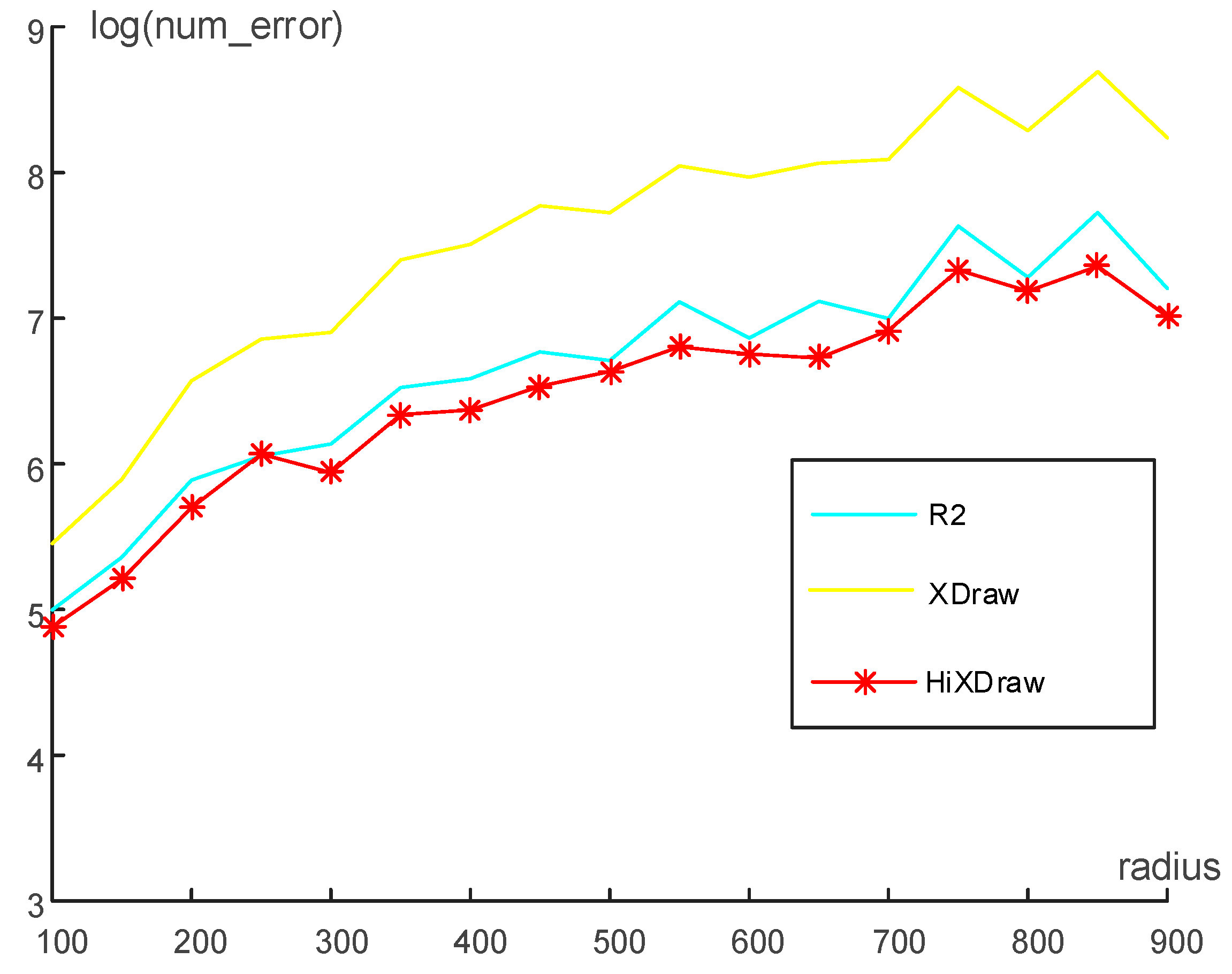
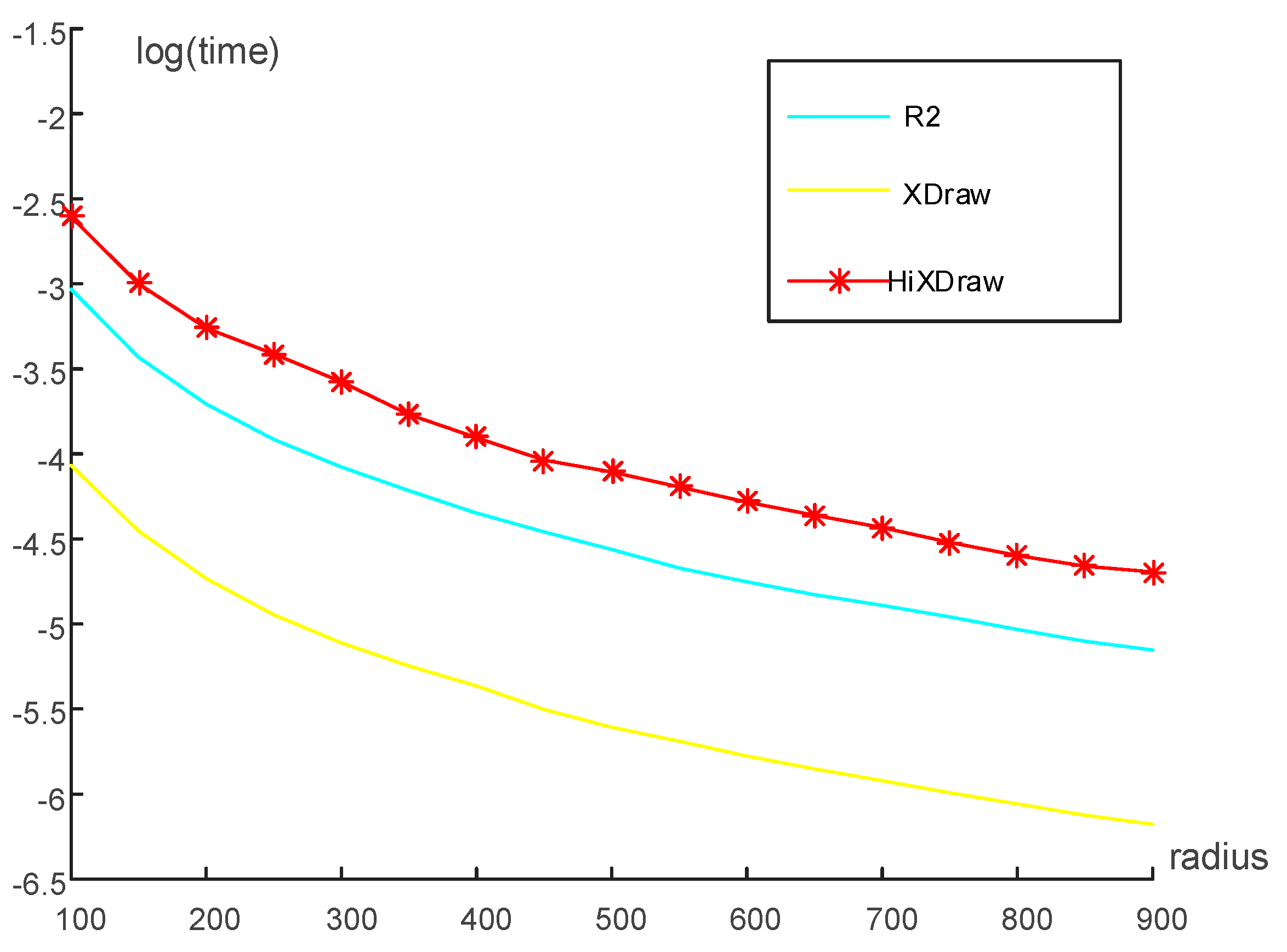
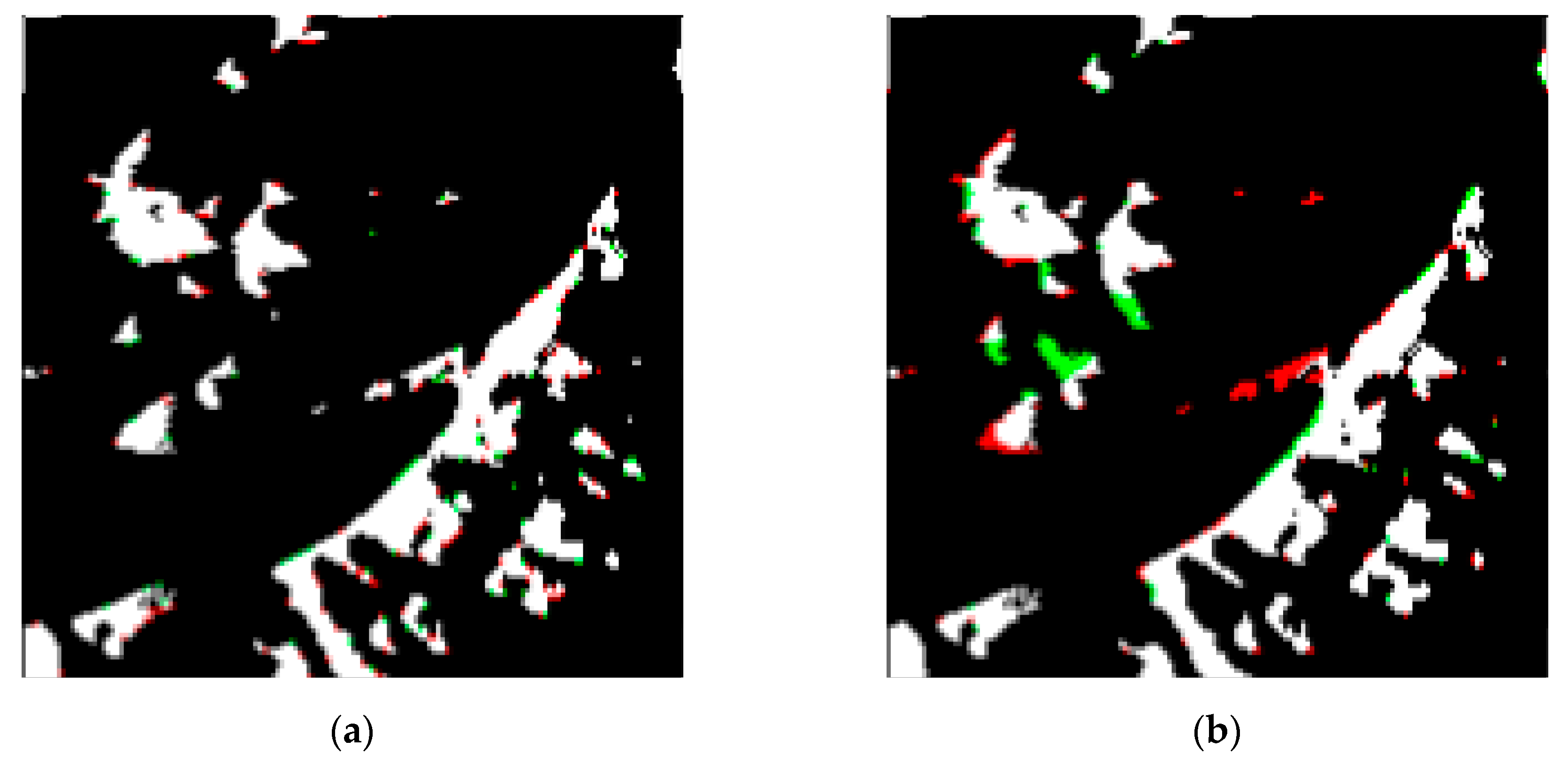
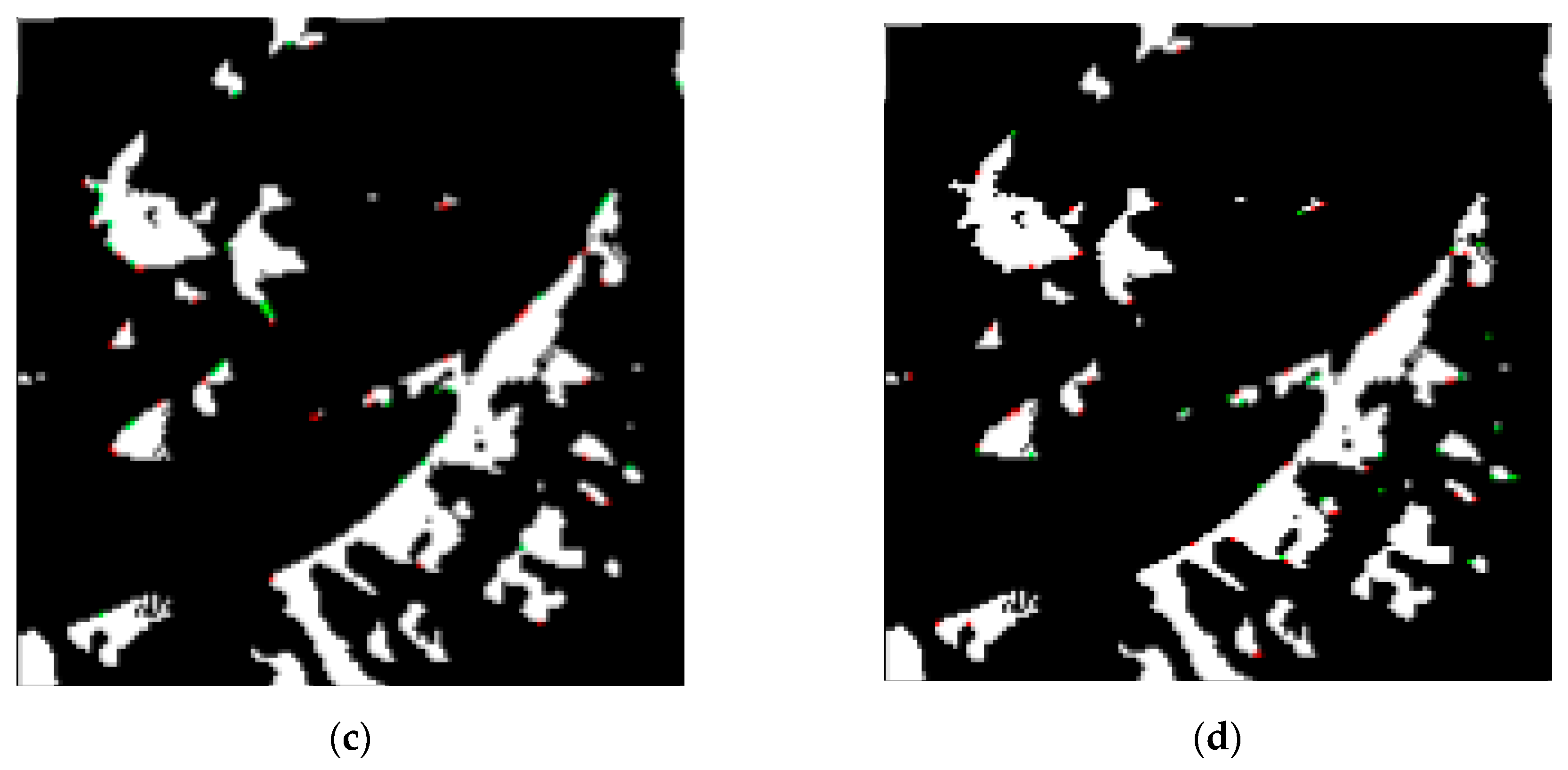
4.2. Experiment 1: Compare the Accuracy and Efficiency of HiXDraw, R2 and XDraw

To assess the accuracy and efficiency of HiXDraw, we apply HiXDraw, R2 and XDraw with different radius and positions. Evaluate the radius every 50 from 100 to 900 in pixels. For each value of radius, we randomly select 100 different positions as viewpoints within the DEM under the premise of ensuring the same analysis area. Figure 5 shows an example of viewpoint selection when radius equals 100. For each position, apply these algorithms to the rectangle analysis area centered at the position. By averaging the data obtained from different positions, we can improve the credibility of the experiment. To access the accuracy performance of various viewshed algorithms, we use the number of error discrimination as an index. To assess the efficiency performance of different algorithms, we use the CPU time as an index. As the outcome curves are very close to each other, we present the statistical data in logarithm to avoid congestion in Figure 6 and Figure 7.

The average number of error discrimination varies with the radius as shown in Figure 6. That the curve is lower means better accuracy. HiXDraw (red) performs better than R2 (cyan) and much better than the original XDraw (yellow).

With the time of R3 being one, Figure 7 shows the relative time of different algorithms in logarithm. The time complexity of R3 is O (r³). The time complexities of other methods, including HiXDraw, are O (r²) with different constant coefficients. XDraw (yellow) is the fastest among these algorithms. HiXDraw (red) is slower than R2 (cyan).

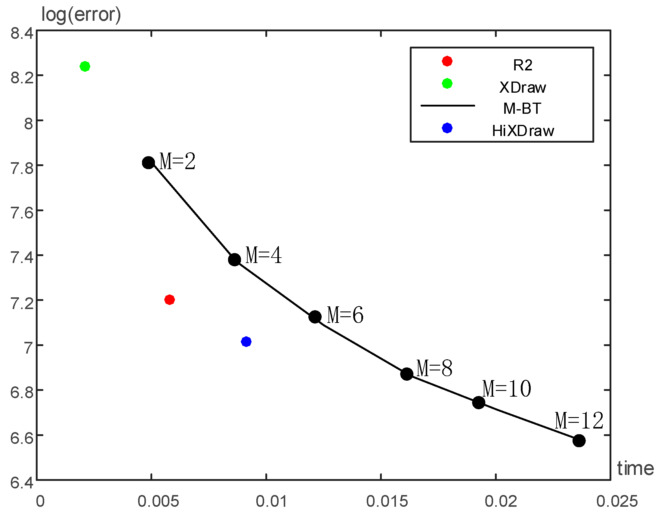
4.3. Experiment 2: Compare the Performance of HiXDraw and M-BT

To compare the performance of HiXDraw and M-BT, we apply M-BT not with different radius but with different backtrack orders. As both the accuracy and efficiency of M-BT depend on its backtrack order M, we execute M-BT with backtrack order of 2, 4, 6, 8, 10 and 12 respectively when radius equals 900 pixels. For each value of M, we randomly select 100 viewpoints and average the time and error among these positions.

Taking both accuracy and efficiency into consideration, Figure 8 illustrates the performance of XDraw, R2, HiXDraw and M-BT. HiXDraw (blue) is more accurate but slower than XDraw (green) and R2 (red). Although M-BT can achieve higher accuracy than HiXDraw with a high backtrack order, HiXDraw takes a shorter time to achieve the same accuracy. Using the same computing time, HiXDraw produces a more accurate viewshed. As a result, HiXDraw performs better than M-BT considering both accuracy and efficiency.

4.4. Experiment 3: Compare the Performance of HiXDraw and Zhi’s Method

Define time ratio η and error ratio μ as (1) and (2):

$$\eta =\frac{1}{n}{\displaystyle {\sum }_{radius}}\frac{time}{tim{e}_{XDraw}}\times 100\%$$

(1)

$$\mu =\frac{1}{n}{\displaystyle {\sum }_{radius}}\frac{error}{erro{r}_{XDraw}}\times 100\%$$

(2)

where n refers to the number of different radii.

Either time ratio η or error ratio μ indicates a better performance with a smaller value. With these two variables, we can access the accuracy and efficiency of HiXDraw, R2 and XDraw statistically. As we did not implement Zhi’s method directly, we use the data recorded in Reference [23] to evaluate the performance of Zhi’s method and make a comparison between HiXDraw and Zhi’s method.

Table 2. The time and error of XDraw, R2 and HiXDraw with different radius.

Algorithms	Radius	100	200	300	400	500	600	700	800	900
XDraw	time 1	1.71	0.88	0.60	0.47	0.37	0.31	0.27	0.23	0.21
	error	233.3	713.6	994.6	1823.7	2261.2	2891.3	3262.7	3977.8	3786.4
R2	time	4.82	2.46	1.70	1.29	1.04	0.86	0.75	065	0.58
	error	147.9	360.8	462.0	724.0	820.5	957.9	1094.6	1452.9	1345.2
HiXDraw	time	7.38	3.84	2.80	2.01	1.65	1.38	1.19	1.01	0.92
	error	131.5	298.7	379.9	583.8	760.6	856.9	1007.5	1320.3	1110.4

¹ time of R3 is 100.The result is ${\eta }_{HiXDraw}\approx 4.4$, ${\mu }_{HiXDraw}\approx 34.96\%$, ${\eta }_{R2}\approx 2.8$, ${\mu }_{R2}\approx 41.85\%$. On average, the error of HiXDraw reduces to 34.96% of XDraw. The computing time is 4.4 times as long as that of XDraw. The accuracy is significantly improved at the cost of more computation. HiXDraw performs better than R2 in terms of accuracy. Using the data given in Reference [23], the result of Zhi’s method is ${\eta }_{Zhi}\approx 9.34$, ${\mu }_{Zhi}\approx 56.91\%$. With twice computing time, Zhi’s method makes more mistakes than HiXDraw. HiXDraw outperforms Zhi’s method in both efficiency and accuracy.

gives the number of errors and the computing time of XDraw, R2 and HiXDraw with different radius. Assume the time of R3 is 100. The relative time of other algorithms reduces with the radius. Using the time ratio η and error ratio μ defined before, we give a statistical assessment on the performance of different viewshed algorithms.

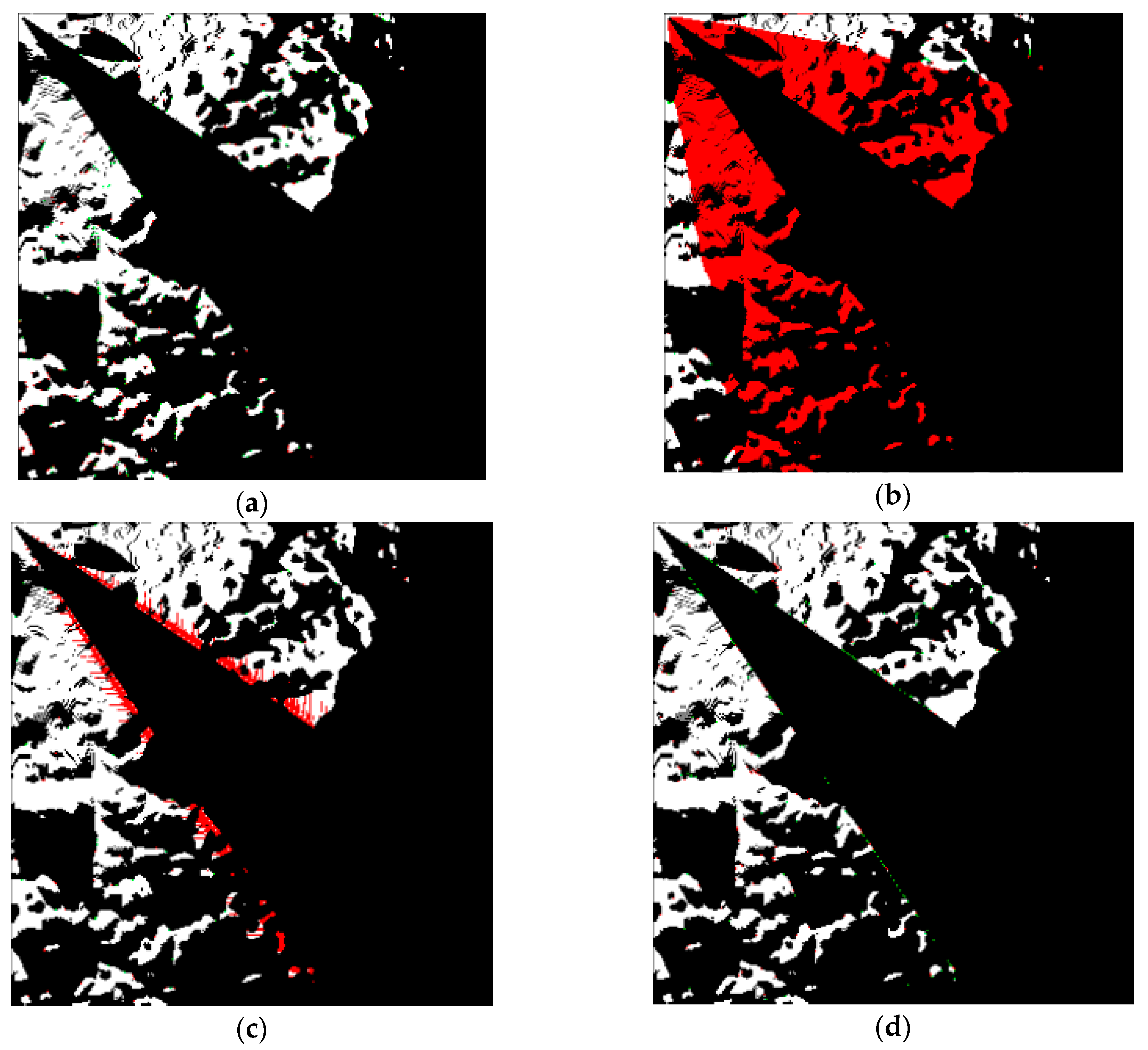
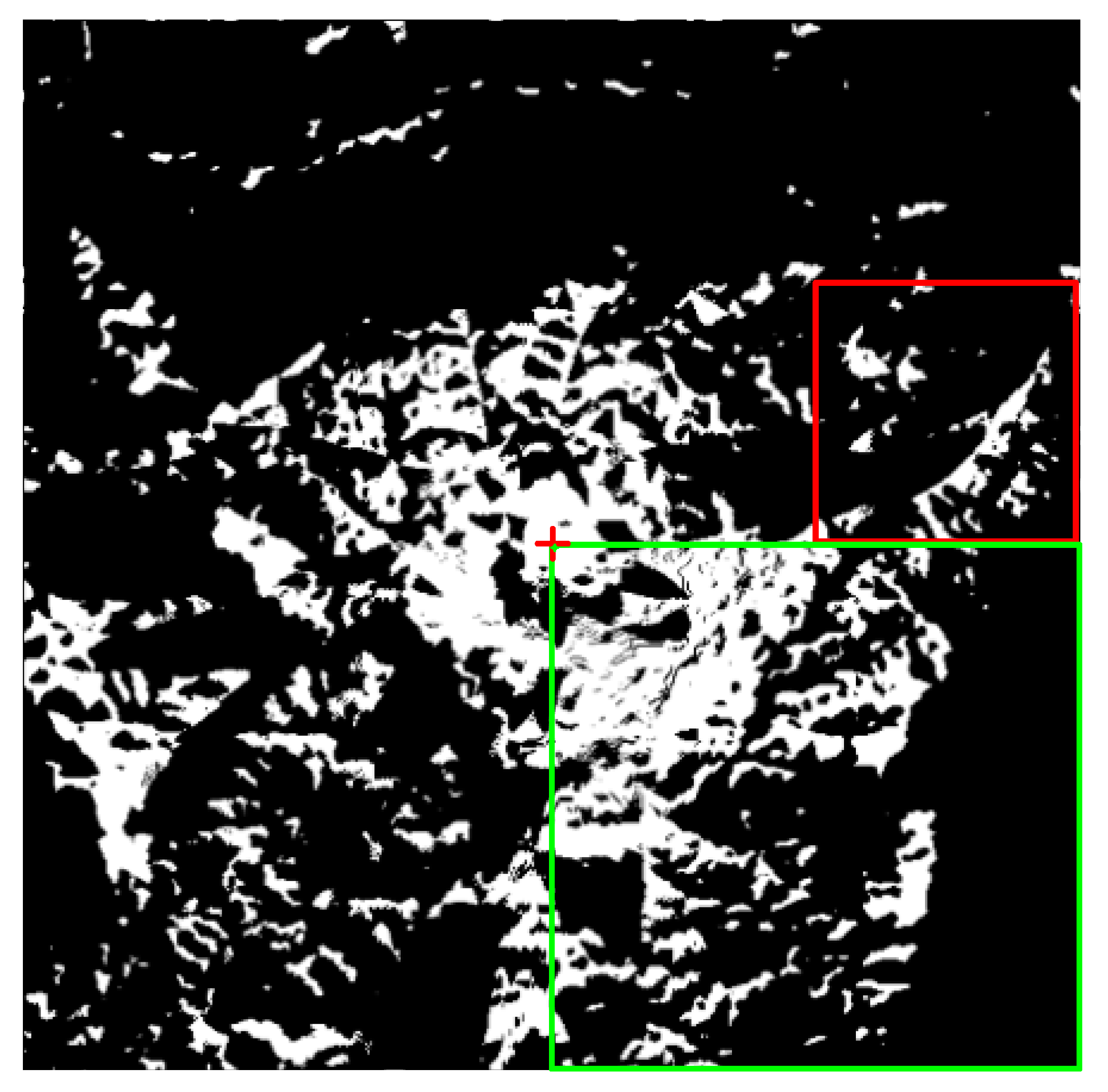
4.5. Experiment 4: A Pillar Experiment

Chunk distortion occurs especially when there is a dominant feature near the viewpoint. To intuitively illustrate the removal of chunk distortion in HiXDraw, we present a pillar experiment with the viewpoint located at (8828, 5717) of the DEM. The radius is 300 pixels and the observer is 30 meters above the ground. We place a pillar as high as 999 meters at (2, 2) southeast to the viewpoint. The diameter of the pillar is one pixel.

Figure 9 shows the viewshed calculated by R3 without a pillar. We highlight the viewpoint with a red plus at the center of the viewshed.

Figure 10 shows the partial viewsheds of the same area corresponding to the red rectangle in Figure 9. It is evident that XDraw has more mistakes than other algorithms. However, the difference between the other three is indistinguishable.

Figure 11 shows the viewsheds of different algorithms within the green rectangle under the influence of a pillar. The viewshed of R2 bears a strong resemblance to that of R3. XDraw wrongly determines a significant fraction of the total target points as invisible. The 10-BT performs better than XDraw but still makes many mistakes under the influence of the extreme height of this pillar. As a contrast, HiXDraw makes few mistakes and successfully eliminates the chunk distortion.

5. Conclusions

We have proposed three propositions to explain the causation of chunk distortion from an innovative contributing perspective. Based on the analysis of chunk distortion, we have devised a new auxiliary grid and the improved XDraw algorithm. As is shown in Section 4, we have improved the accuracy of XDraw significantly and we have eliminated chunk distortion in XDraw. The error rate of HiXDraw reduces to 34.96% of the original XDraw, which is lower than 41.85% of R2 and much lower than 56.91% of Zhi’s method. Using the same computing time, the error rate of HiXDraw is also lower than that of M-BT. The computing time of HiXDraw is 4.4 times as long as that of XDraw, slightly longer than R2 (2.8 times) and less than half of Zhi’s method (9.34 times). Generally, HiXDraw performs comparably to other algorithms in terms of efficiency. While M-BT and Zhi’s method failed to eradicate chunk distortion, HiXDraw has successfully eliminated chunk distortion. The shortcomings of HiXDraw mainly lie in three aspects:

More memory: HiXDraw requires more memory to record contributing points at invisible points. The new auxiliary grid does not record the LOS height but the contributing points. By recording two contributing points at invisible points, we can obtain the LOS height by reconstructing the reference plane using the contributing points. However, we cannot reconstruct the reference plane from the LOS height, because two reference points that form this plane are unknown. This indicates that by recording LOS height only, we lose partial LOS information. The new auxiliary grid requires more memory to take down detailed LOS information. Note that with the new auxiliary grid, HiXDraw uses only the actual elevations to construct a reference plane. Although More memory is used, the improvement in accuracy makes it worthwhile.

More computation (longer computing time): HiXDraw involves more computation to generate a viewshed. The contributing points used to construct the reference plane are selected from at most four contributing points. These two points are no longer in the same column or row. Their position can be arbitrary. It means we require more computation for a single target when we use a coplanar equation to compute the minimum visible elevation. Also, selecting contributing points requires extra computation. The computation time in our experiment is averagely 4.4 times as long as that of XDraw. Again, HiXDraw performs comparably to other algorithms in terms of efficiency. Moreover, the improvement in accuracy has proved the merits of involving more calculation.

Few violations of the criteria for appropriateness: By constraining the contributing points “adjacent” to LOS, HiXDraw avoids the unwanted dependency propagation. However, it occasionally occurs in the experiment when the contributing point with the smallest angle is more than distance one away from LOS. In this case, HiXDraw violates the criteria for appropriateness. This phenomenon indicates that this work can be improved further in the future. In most cases, the selected contributing points locate within 4-neighborhood of LOS.

In this paper, we have proposed HiXDraw—an improved XDraw algorithm free of chunk distortion. We have explained the causation for chunk distortion with three propositions from a contributing perspective. We have devised a new auxiliary grid recording not the LOS height but the contributing points at invisible target points. By choosing the most “adjacent” contributing points, we have terminated the pervasive dependency propagation and have eliminated the chunk distortion. As a result, HiXDraw improves the accuracy of outcome viewshed significantly. Error rate reduces to around one-third of the original XDraw.

6. Future works

Some directions for future research include:

• (Better efficiency) Speed up HiXDraw with an I/O efficient operation and parallel computing. As we have mentioned in Section 2, many previous works had accelerated the original XDraw by implementing XDraw I/O-efficiently or by adapting XDraw to various parallel technologies. HiXDraw does not change the overall procedure of XDraw, making it possible to apply the speed up to the new method easily.
• (Better accuracy) Improve the selection of contributing points with a more reasonable criterion. The criteria for choosing contributing points is open for further discussion. Other criteria considering more factors other than azimuth can be proposed to achieve better performance. For example, suppose one of the contributing points has the smallest angle but another contributing point is closest to the viewpoint and is much more dominant, should we ignore the influence of the dominant point? How to consider the influence of all the candidate contributing points comprehensively? Whether other points, such as the invisible reference points, should be included in the consideration? Future works should examine other factors and design new criteria.
• (Better accuracy) Besides, involving other “relevant” terrain data into the computation of visibility may be another direction of improving accuracy. By constructing the reference plane using two reference points and the viewpoint, XDraw assumes that the reference plane is higher than all the grid points within this triangle. Unfortunately, this assumption is not always correct. [31] illustrated a counterexample. We may solve this problem by taking more terrain data along the LOS into consideration.
• (More applications) The contributing points used to construct the reference plane is no longer in the same row or column. The position of the contributing point is arbitrary. So there exists a possibility that we may apply HiXDraw to TIN terrain models in the future.

References

1. Franklin, W.R.; Ray, C.K.; Mehta, S. Geometric algorithms for siting of air defense missile batteries. Res. Proj. Battle Columb. Div. Deliv. Order 1994, 2756. [Google Scholar]
2. Li, J.; Zheng, C.; Hu, X. An Effective Method for Complete Visual Coverage Path Planning. In Proceedings of the 2010 Third International Joint Conference on Computational Science and Optimization (CSO), Huangshan, China, 28–31 May 2010; Volume 1, pp. 497–500. [Google Scholar]
3. Yaagoubi, R.; Yarmani, M.E.; Kamel, A.; Khemiri, W. HybVOR: A voronoi-based 3D GIS approach for camera surveillance network placement. ISPRS Int. J. Geo-Inf. 2015, 4, 754–782. [Google Scholar] [CrossRef]
4. Kaučič, B.; Zalik, B. Comparison of viewshed algorithms on regular spaced points. In Proceedings of the 18th Spring Conference on Computer Graphics, Budmerice, Slovakia, 24–27 April 2002; ACM: New York, NY, USA, 2002; pp. 177–183. [Google Scholar]
5. Teng, Y.A.; Davis, L.S. Visibility Analysis on Digital Terrain Models and Its Parallel Implementation; University of Maryland, Center for Automation Research, Computer Vision Laboratory: College Park, MD, USA, 1992. [Google Scholar]
6. Toma, L. Viewsheds on terrains in external memory. Sigspatial Spec. 2012, 4, 13–17. [Google Scholar] [CrossRef]
7. Van Kreveld, M.J. Variations on Sweep Algorithms: Efficient Computation of Extended Viewsheds and Class Intervals; Utrecht University, Information and Computing Sciences: Utrecht, The Netherlands, 1996. [Google Scholar]
8. Or, D.C.; Shaked, A. Visibility and Dead-Zones in Digital Terrain Maps. In Computer Graphics Forum; Blackwell Science Ltd.: Edinburgh, UK, 1995; Volume 14, pp. 171–180. [Google Scholar]
9. Fishman, J.; Haverkort, H.; Toma, L. Improved visibility computation on massive grid terrains. In Proceedings of the 17th ACM SIGSPATIAL International Conference on Advances in Geographic Information Systems, Seattle, WD, USA, 4–6 November 2009; ACM: New York, NY, USA, 2009; pp. 121–130. [Google Scholar]
10. Haverkort, H.; Toma, L. A Comparison of I/O-Efficient Algorithms for Visibility Computation on Massive Grid Terrains. arXiv, 2018; arXiv:1810.01946. [Google Scholar]
11. Haverkort, H.; Toma, L.; Zhuang, Y. Computing visibility on terrains in external memory. J. Exp. Algorithmics (Jea) 2009, 13, 5. [Google Scholar] [CrossRef]
12. Ferreira, C.R.; Andrade, M.V.A.; Magalhaes, S.V.G.; Franklin, W.R. An efficient external memory algorithm for terrain viewshed computation. ACM Trans. Spat. Algorithms Syst. (TSAS) 2016, 2, 6. [Google Scholar] [CrossRef]
13. Haverkort, H.; Toma, L.; Wei, B.P.F. On IO-efficient viewshed algorithms and their accuracy. In Proceedings of the 21st ACM SIGSPATIAL International Conference on Advances in Geographic Information Systems, Orlando, FL, USA, 5–8 Npvember 2013; ACM: New York, NY, USA, 2013; pp. 24–33. [Google Scholar]
14. Ferreira, C.R.; Magalhães, S.V.; Andrade, M.V.; Franklin, W.R.; Pompermayer, A.M. More efficient terrain viewshed computation on massive datasets using external memory. In Proceedings of the 20th International Conference on Advances in Geographic Information Systems, Redondo Beach, CA, USA, 6–9 November 2012; ACM: New York, NY, USA, 2012; pp. 494–497. [Google Scholar]
15. Osterman, A.; Benedičič, L.; Ritoša, P. An IO-efficient parallel implementation of an R2 viewshed algorithm for large terrain maps on a CUDA GPU. Int. J. Geogr. Inf. Sci. 2014, 28, 2304–2327. [Google Scholar] [CrossRef]
16. Axell, T.; Fridén, M. Comparison between GPU and Parallel CPU Optimizations in Viewshed Analysis. Master’s Thesis, Department of Computer Science and Engineering, Chalmers University of Technology, Gothenburg, Sweden, 2015. [Google Scholar]
17. Zhao, Y.; Padmanabhan, A.; Wang, S. A parallel computing approach to viewshed analysis of large terrain data using graphics processing units. Int. J. Geogr. Inf. Sci. 2013, 27, 363–384. [Google Scholar] [CrossRef]
18. Ferreira, C.; Andrade, M.V.; Magalhães, S.V.; Franklin, W.R.; Pena, G.C. A Parallel Sweep Line Algorithm for Visibility Computation; GeoInfo: São Paulo, Brazil, 2013; pp. 85–96. [Google Scholar]
19. Ferreira, C.R.; Andrade, M.V.; Magalhães, S.V.; Franklin, W.R.; Pena, G.C. A parallel algorithm for viewshed computation on grid terrains. J. Inf. Data Manag. 2014, 5, 171. [Google Scholar]
20. Dou, W.; Li, Y.; Wang, Y. A fine-granularity scheduling algorithm for parallel XDraw viewshed analysis. Earth Sci. Inform. 2018, 1–15. [Google Scholar] [CrossRef]
21. Wang, J.; Robinson, G.J.; White, K. Generating viewsheds without using sightlines. Photogramm. Eng. Remote Sens. 2000, 66, 87–90. [Google Scholar]
22. Izraelevitz, D. A fast algorithm for approximate viewshed computation. Photogramm. Eng. Remote Sens. 2003, 69, 767–774. [Google Scholar] [CrossRef]
23. Zhi, Y.; Wu, L.; Sui, Z.; Cai, H. An improved algorithm for computing viewshed based on reference planes. In Proceedings of the IEEE 2011 19th International Conference on Geoinformatics, Shanghai, China, 24–26 June 2011; pp. 1–5. [Google Scholar]
24. Wu, H.; Pan, M.; Yao, L.; Luo, B. A partition-based serial algorithm for generating viewshed on massive DEMs. Int. J. Geogr. Inf. Sci. 2007, 21, 955–964. [Google Scholar] [CrossRef]
25. Xu, Z.Y.; Yao, Q. A novel algorithm for viewshed based on digital elevation model. In Proceedings of the Asia-Pacific Conference on Information Processing (APCIP 2009), Shenzhen, China, 18–19 July 2009; Volume 2, pp. 294–297. [Google Scholar]
26. Carabaño, J.; Sarjakoski, T.; Westerholm, J. Efficient implementation of a fast viewshed algorithm on SIMD architectures. In Proceedings of the Proceedings of the 23rd Euromicro International Conference on Parallel, Disturbed, and Network-Based Processing, Turku, Finland, 4–6 March 2015. [Google Scholar]
27. Cauchi-Saunders, A.J.; Lewis, I.J. GPU enabled XDraw viewshed analysis. J. Parallel Distrib. Comput. 2015, 84, 87–93. [Google Scholar] [CrossRef]
28. Song, X.D.; Tang, G.A.; Liu, X.J.; Dou, W.F.; Li, F.Y. Parallel viewshed analysis on a PC cluster system using triple-based irregular partition scheme. Earth Sci. Inform. 2016, 9, 511–523. [Google Scholar] [CrossRef]
29. Li, Y.N.; Dou, W.F.; Wang, Y.L. Design and Implementation of parallel XDraw algorithm based on triangle region division. In Proceedings of the 2017 16th International Symposium on Distributed Computing and Applications to Business, Engineering and Science (DCABES), AnYang, China, 13–16 October 2017; pp. 41–44. [Google Scholar]
30. Dou, W.; Li, Y. A fault-tolerant computing method for Xdraw parallel algorithm. J. Supercomput. 2018, 74, 2776–2800. [Google Scholar] [CrossRef]
31. Yu, J.; Wu, L.; Hu, Q.; Yan, Z.; Zhang, S. A synthetic visual plane algorithm for visibility computation in consideration of accuracy and efficiency. Comput. Geosci. 2017, 109, 315–322. [Google Scholar] [CrossRef]
Figure 1. The direct LOS method and the LOS height. The curve represents the profile of a terrain. v is the viewpoint above the terrain. t1 and t2 are two adjacent targets on the terrain. The direct LOS method determines the visibility of a target point by comparing its predicted minimum visible height and its elevation. The elevation of t1 is higher than its predicted minimum visible height. t1 is visible and t1’s LOS height H1 equals the actual elevation of t1. The elevation of t2 is lower than its predicted minimum visible elevation. t2 is invisible and its LOS height H2 equals the minimum visible height.
Ijgi 08 00153 g001
Figure 2. The procedure of XDraw. First, XDraw assumes that the eight neighboring points near the viewpoint are visible. Second, XDraw applies the direct LOS method on the eight directions (vertical, horizontal and diagonal directions). Finally, for targets in eight octants, XDraw determines the visibility in layers from the viewpoint to the boundary of the analysis area. Each target relies on two reference points on the previous layer to calculate the visibility.
Ijgi 08 00153 g002
Figure 3. Only partial visible points in the dependency parallelogram influence the visibility computation of the target point. (a) demonstrates the relative positions of viewpoint v and target point t on a 2D grid. Suppose a vertical screen stands on the right edge of the grid and is perpendicular to the grid, (b) illustrates the result of the perspective projection of (a) originated at viewpoint onto the screen. (a,b) together show how the points in the dependency parallelogram contribute to the visibility of the target.
Ijgi 08 00153 g003
Figure 4. The number of contributing points. v is the viewpoint. t is the target point. A rectangle point represents a visible point and a round point represents an invisible point. (a) t’s two reference points, P42 and P43, are both visible. t has two contributing points: P42 and P43; (b) one of t’s reference points, P43, is invisible. Suppose the contributing points of P43 are P33 and P32. t has three contributing points: P42, P32 and P33; (c) t’s two reference points, P43 and P42, are both invisible. Suppose the contributing points of P43 is P33 and P32. Suppose the contributing points of P42 is P32 and P31. P43 and P42 share a common contributing point P32. t has three contributing points: P31, P32 and P33; (d) one of t’s reference points P31 is invisible. Suppose the contributing points of P31 is P21 and P20. t has three contributing points: P20, P21 and P32. P21 lies right on the LOS of t.
Ijgi 08 00153 g004
Figure 5. A 11264 by 9152 DEM of a mountainous area in Hunan Province, China. Randomly select 100 positions when the radius equals 100.
Ijgi 08 00153 g005
Figure 6. The number of error discrimination in logarithm. HiXDraw (red) performs better than R2 (cyan) and much better than the original XDraw (yellow) concerning accuracy.
Ijgi 08 00153 g006
Figure 7. The relative CPU time of different algorithms in logarithm. HiXDraw (red) is slower than XDraw (yellow) and R2 (cyan).
Ijgi 08 00153 g007
Figure 8. Comparison of different algorithms taking both accuracy and efficiency into consideration. Assume the time of R3 is one. The x-axis represents the relative time used by each algorithm. The y-axis represents the number of error determinations in logarithm. The performance of M-BT (black) varies with backtrack order from two to twelve. HiXDraw (blue) is more accurate but slower than XDraw (green) and R2 (red). Although M-BT can achieve higher accuracy with a high backtrack order, HiXDraw expends shorter time achieving the same accuracy.
Ijgi 08 00153 g008
Figure 9. Viewshed generated by R3 with a viewpoint located at the center. The radius of the analysis area is 300 and the observer is 30 meters above the ground.
Ijgi 08 00153 g009
Figure 10. Partial viewsheds of different algorithms corresponding to the red rectangle in Figure 9. These viewsheds are generated by (a) R2, (b) XDraw, (c) 10-BT and (d) HiXDraw, respectively. Red means visible areas are wrongly determined as invisible and green means invisible areas are wrongly determined as visible.
Ijgi 08 00153 g010aIjgi 08 00153 g010b
Figure 11. Partial viewsheds under the influence of a pillar corresponding to the green rectangle in Figure 9. The pillar of 999 meters high is placed at (2, 2) southeast to the viewpoint. These viewsheds are generated by (a) R2, (b) XDraw, (c) 10-BT and (d) HiXDraw, respectively. Red means visible areas are wrongly determined as invisible and green means invisible areas are wrongly determined as visible.
Ijgi 08 00153 g011