Abstract
Landscape metrics constitute one of the main tools for the study of the changes of the landscape and of the ecological structure of a region. The most popular software for landscape metrics evaluation is FRAGSTATS, which is free to use but does not have free or open source software (FOSS). Therefore, FOSS implementations, such as QGIS’s LecoS plugin and GRASS’ r.li modules suite, were developed. While metrics are defined in the same way, the “cell neighborhood” parameter, specifying the configuration of the moving window used for the analysis, is managed differently: FRAGSTATS can use values of 4 or 8 (8 is default), LecoS uses 8 and r.li 4. Tests were performed to evaluate the landscape metrics variability depending on the “cell neighborhood” values: some metrics, such as “edge density” and “landscape shape index”, do not change, other, for example “patch number”, “patch density”, and “mean patch area”, vary up to 100% for real maps and 500% for maps built to highlight this variation. A review of the scientific literature was carried out to check how often the value of the “cell neighborhood” parameter is explicitly declared. A method based on the “aggregation index” is proposed to estimate the effect of the uncertainty on the “cell neighborhood” parameter on landscape metrics for different maps.
1. Introduction
In recent decades, landscape metrics were one of the main tools for the study, quantification, and possibly the parametrization of the changes of the landscape and of the ecological structure of a territory [1,2]. Landscapes consist of natural or anthropogenically modified mosaics of patches, and the spatial arrangement of these patches is called landscape pattern [3]. The quantification of spatial heterogeneity over multiple spatial and temporal scales is necessary to clarify the relationships between ecological processes and spatial patterns [4,5]. Landscape metrics became standard and gained the status of an indispensable instrument for those who investigate landscape change dynamics not only in ecology [6,7] but also in many other disciplines such as soil protection and water management [8,9,10]. Many are metrics that can be calculated, but some of them are considered particularly robust and significant and are used more frequently in scientific literature [2,6]. It is a common practice to compare the different landscapes according to the results of some of these indices like, for example, patch number (NP) or mean patch size (MPS) [11]. However, we argue that the results of some of the most used and reliable indices can be severely affected by the settings used during the processing [11] and, if these settings are not accurately described in the scientific works, this can create a cascade effect that affects the comparability of the results. In particular, we realized that the cell neighborhood size is one of the most sensible parameters but a literature analysis highlighted that not many works have investigated its influence. Additionally, each software provides information about the setting of cell neighborhood size with different emphasis.
The most popular software for landscape metrics evaluation is FRAGSTATS [12], which is free to use but not free or open source software (FOSS). Therefore, FOSS implementations, such as QGIS’s LecoS plugin and GRASS’ r.li modules suite, were developed. Landscape metrics are defined in the same way in all these software. However, the cell neighborhood parameter, specifying the configuration of the moving window used for the analysis, is managed differently: FRAGSTATS can use values of 4 or 8 (8 is default), LecoS uses 8 and r.li 4.
Are the software users aware of which cell neighborhood size they are using and what the performances and the effects it can produce are? How reliable are the comparisons among different studies that do not mention the cell neighborhood size settings? Is it possible to safely compare the results of works carried out with different software?
In order to answer to these questions the aims of our work are: (i) to investigate how the cell neighborhood size affects the results of landscape metrics calculation using both tests map and real maps; (ii) to examine the transparency of the settings of the cell neighborhood size in different software; (iii) to understand if the cell neighborhood size settings are usually reported in the scientific papers and, therefore, how reliable are the comparisons of different works developed with the same or different software.
The paper is organized as follows: Section 2 illustrates the literature review and its results; Section 3 describes the materials and methods used for the analysis, the software, the metrics, and the maps used for the tests; Section 4 illustrates the results; Section 5 describes a new method to evaluate the sensitivity of landscape metrics to the cell neighborhood size and finally the conclusions and future developments are presented in Section 6.
2. Literature Review
An analysis of the scientific literature for papers regarding the use of FRAGSTATS, the LecoS add-on, or the r.li/r.le modules in GRASS GIS was carried out to determine if the cell neighborhood parameter was mentioned or explained in scientific papers describing applications using landscape metrics.
The Scopus database was used, searching for the term “cell neighborhood” coupled with “Fragstats”, “r.li”, “r.le”, “LecoS”, “landscape patch”, and “landscape metrics” as keywords. The joint use of these terms yielded no results, so the keywords have been used separately.
The papers for the current review were chosen following these conditions: (i) the articles must be research papers, peer reviewed, although with no minimum limit on the number of citations; (ii) at least one of the FRAGSTATS, LecoS, or r.li/r.le software must have been used in the study; (iii) more than one landscape metric must have been used; (iv) no limit has been set for the year of publication.
In the Scopus archive the term “landscape metrics” produces an excess of 37,000 results. Refining the search by adding the keyword “Fragstat” narrows the result to 800 papers. Adding the terms “lecos” and“landscape metrics” refines the result to six papers; finally, adding “landscape metrics” with “r.li” refines the result to four papers.
For further analysis the pool of results was narrowed to 93 papers:
- 70 (65.1%) papers cited FRAGSTATS as software for the evaluation of landscape metrics;
- 16 (14.9%) papers cited LecoS as QGIS add-on used for the calculation of the landscape metrics;
- Four (3.7%) papers cited r.li/r.le as GRASS modules for the assessment of the metrics;
- Three (2.8%) papers cited other software for the assessment of the metrics;
- Two papers developed new software for the evaluation of landscape metrics, using as reference for the calculations FRAGSTATS (these papers have been counted in the 70 articles citing FRAGSTATS).
Figure 1 shows the distribution of the software used for landscape analysis in the examined papers.
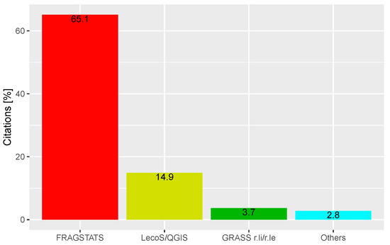
Figure 1.
Comparison of the times each landscape analysis software is cited in the analyzed papers.
These papers can be classified according to their purpose:
- papers that deal with landscape fragmentation as an issue in itself;
- papers that deal with landscape fragmentation as an issue for habitat connectivity;
- papers that investigate which landscape metric could explain other metrics;
- papers that investigate the size of a moving window algorithm and how it affects landscape analysis;
- papers that present new software for landscape metrics calculation, basing their structure and methods on FRAGSTATS.
Table 1 shows the most used landscape metrics, with the numbers of times the selected metric was used in the reviewed papers as absolute values and percentages.

Table 1.
Number and percentage of papers in the analyzed set citing landscape metrics.
Additionally, the number of times nine other metrics are indicated in the set of papers was counted: Largest patch index (34, 37%), Shannon Index (35, 38%), Simpson Index (18, 19.6%), Percentage of landscape (28, 30.4%), Perimeter/Area ratio (20, 21.7%), Euclidean distance (14, 15%), Total edge (27, 29.3%), Shape index (32, 34.8%), Fractal index (22, 23.9%), and Mean nearest neighbor (25, 27.2%).
The value of the cell neighborhood parameter was specified in eight different papers: seven chose a Moore definition [13,14,15,16,17,18,19,20] and one a von Neumann definition [21]. The 16 papers which exclusively employed LecoS [22,23,24,25,26,27,28,29,30,31,32,33,34,35,36,37] used an 8-cells neighborhood rule, as it is the only setting available in the add-on; a similar hypothesis is applicable to the four works which used r.li in GRASS [38,39,40,41], which uses a 4-cells neighborhood definition. The papers which did not specify the definition of the neighborhood in FRAGSTATS are assumed to have used a 8-cells definition, since this is the default setting [42], although it is not possible to prove this assumption. Results in Section 4 demonstrate that some of the most commonly used metrics are affected by the choice of this parameter. Therefore, the fact that the cell neighborhood configuration is not explicitly or implicitly specified in most of the research papers analyzed (by the indication of the software used) could make the results difficult to repeat and interpret.
The full list of the examined papers, a table indicating the papers citing each software, and a breakdown of the landscape metrics cited by each paper is available as an additional material of this paper (see Supplementary Materials).
3. Materials and Methods
To analyze the effect of the cell neighborhood size on the values of landscape metrics calculation, three different geographic information system (GIS) software were selected (Section 3.1) to evaluate a common set of metrics (Section 3.2) on artificial (Section 3.3) and real (Section 3.4) maps.
3.1. Test Software
Tests on artificial (Section 3.3) and real (Section 3.4) maps were carried out using three different software systems: FRAGSTATS [12], GRASS GIS [43], and QGIS [44]. The rationale behind this choice is that using software in the public domain (FRAGSTATS) or available as free and open software (FOSS) (GRASS GIS and QGIS) allows the replication of the experiments described in this paper. Additionally, FOSS source code is available for analysis. Therefore, possible discrepancies between metrics’ values can be resolved examining the code.
According to its manual [45], “FRAGSTATS is a spatial pattern analysis program for quantifying the structure (i.e., composition and configuration) of landscapes.”. FRAGSTATS [12] was the reference software for the evaluation of landscape metrics since its inception in 1995. It is available as executable in the public domain for the MS Windows operative system only. Written in Microsoft Visual C++, the use of a 32-bit address space limits its capacity to process large maps. Its source code is not accessible but its features are well documented in the manual available on-line and its widespread use in landscape and ecology research speaks to its accuracy and reliability in metrics evaluation. Units of input maps are assumed to be meters. Input map can only contain signed integer values and have square cells with sides larger than m. FRAGSTATS can evaluate 36 area and edge metrics, 79 shape metrics, 46 core area metrics, 17 contrast metrics, and 64 aggregation metrics, for a total of 242 different metrics and 392 parameters describing them [45]. Additionally, FRAGSTATS can evaluate 9 Diversity Metrics.
GRASS GIS [43] is a multi-purpose FOSS GIS for geospatial data production, analysis, and mapping [46] available under the GNU Public License (GPL), used in research and education [47]. It is part of the Open Source Geospatial Foundation (OSGeo). GRASS is mainly written in ANSI C, with some parts in the C++ and, more recently, in the Python programming languages; it is highly modular and easily scriptable. Besides the source code, it is available as ready to install packages for the MS Windows, Apple Mac OSX, and Linux operating systems. Limitations on data size are mostly related to the capacity of the operative system to deal with large files [48], with the possibility of enabling large file support (LFS). Landscape analysis in GRASS is carried out using the r.li modules suite, which can evaluate 10 patch indices and 7 diversity indices and provides a graphical user interface for the configuration of the analysis. A previous implementation of landscape metrics evaluation, called r.le is used in old GRASS versions.
QGIS is a user friendly open source geographic information system (GIS) licensed under the GNU General Public License [44], part of the Open Source Geospatial Foundation (OSGeo). It is written in the C++ language using the Qt toolkit for its interface. Plugins can be written either in C++ or Python. It is available as source code and packages for the Linux, Unix, Mac OSX, MS Windows, and Android operative systems. The maximum size for maps depends on the combination of operative system and Geospatial Data Abstraction Library (GDAL)/OGR Simple Features Library (OGR) limitations for the data type in use. The Landscape ecology statistics (LecoS) plugin performs landscape analysis in QGIS using the Python numpy library [49]. LecoS, like version 3.0.0, can evaluate 20 landscape metrics, 8 zonal statistics and 3 diversity indexes.
Other modules to calculate landscape metrics are integrated in the most popular GIS desktop software: V-Late and PA4 in ArcGIS (set of GIS programs created by the Environmental Systems Research Institute, ESRI), Pattern and Texture modules in IDRISI, and the API called Land-metrics DIY developed by Zaragozí et al. [50] and released under the GPL license. Recently, a new R package dedicated to calculation of landscape metrics was released; with landscapemetrics it is now possible to perform landscape analysis on rasters inside the R environment [51].
FRAGSTATS 4.2, GRASS 7.6, and QGIS 3.4 (LecoS 3.0.0) versions were used for the tests. A comprehensive list of the software features with respect to landscape metrics is reported in Appendix A.
3.2. Landscape Metrics
Landscape metrics are indexes used to describe and quantify the spatial characteristics of the landscape, described as a set of categorical data, typically representing land use [6]. These indexes are useful to study the evolution of the landscape features over time [7,41,52,53] or to compare different areas [6].
The great variety of metrics can be classified according to the spatial level they are dealing with: patches, classes of patches, or the whole landscape [54]. Commonly, in landscape ecology, a patch is defined as a discrete area of homogeneous environmental conditions at a specific scale [45]. These metrics fall into two categories: those that quantify the composition of the map without reference to spatial attributes (for example, the number of patches) and those that quantify the spatial configuration of the map, such as spatial arrangement, position, or orientation of the patches [54].
Landscape metrics calculated at the patch level describe simple statistics about each land use patch (area, perimeter, number of patches, …) and serve primarily as the computational basis for other landscape metrics [45]. Landscape metrics calculated at the class level report information about all the patches of a given type. These metrics are useful to quantify the amount and spatial configuration of each patch type and thus are useful to estimate the fragmentation of each patch type in the landscape [45]. Finally, landscape metrics can provide information about the pattern, like class metrics: these may be integrated by a simple or weighted averaging or may reflect aggregate properties of the patch mosaic [45].
For the purpose of this work, a limited number of landscape metrics was selected among the many available according to the following criteria: (i) the availability for calculation across software; (ii) the use of the cell neighborhood parameter for their calculation; (iii) the relative simplicity of their formulation, in order to understand the effect of the cell neighbor parameter on the result and to be able to manually evaluate their values for simple maps.
- Patch Number (NP)
- is the number of patches of each type; it is an adimensional metric. It is defined as:where:
- N is the number of patches in the k-th category.
- Patch density (PD)
- equals the number of patches of the corresponding patch type divided by total landscape area [m], multiplied by 10,000 and 100 (to convert to 100 hectares). The unit of measure is number of patches per 100 hectares. It is expressed as:where:
- N is the number of patches in the landscape;
- A is the total landscape area in [m];
- and 100 are constant and used to express the index in (100) ha.
- Mean patch size (MPS)
- is the average area of all the patches of a given type. It is measured in square meters. When used in combination with NP, MPS gives information about how the patches of a given land use class are growing or merging over time [53]. It is defined as:where:
- A is the area of the patches in [m];
- is the number of patches.
- Edge density (ED)
- equals the sum of the lengths (m) of all edge segments involving the corresponding patch type, divided by the total landscape area (m), multiplied by 10,000 (to convert to hectares). The unit is meters per hectare. ED > 0. This index is useful in ecological studies dealing with ecotone species. It is expressed as:where:
- k is the category of the patches;
- m is the total number of different categories of patches;
- n is the number of boundary edges for the patch;
- is the total length of boundary edges for the k-th category of patches;
- A is the total landscape area;
- is a constant to convert the index in [m/ha].
- Landscape shape index (LSI)
- measures the perimeter-to-area ratio for the landscape as a whole. All edge segments (m) within the landscape boundary involving the corresponding patch type are divided by the square root of the total landscape area (m). LSI > 1, adimensional. This index is a measure of the overall geometric complexity of the landscape and is defined as:where:
- E is the sum of the lengths of all the boundary edges of the patches;
- A is the sum of all the areas of the patches;
- 0.25 is a adjustment coefficient.
- Aggregation index (AI)
- equals the number of adjacent patches involving the corresponding class, divided by the maximum possible number of like adjacencies, which is achieved when the class is maximally clumped into a single, compact patch, multiplied the proportion of the landscape comprised of the corresponding class, summed over all classes and multiplied by 100 (to convert to a percentage). Unit: Percent, range 0 < AI < 100 [45]. It is useful to quantify spatial patterns and fragmentation of the landscape. It is defined as:where:
- is the number of like adjacencies between pixels of patch class i based on the single-count method;
- is the maximum number of like adjacencies between pixels of patch class i based on the single-count method;
- 100 is a constant used to express the index as percentage.
Cell neighborhood is defined as the nearest cells to a specific one. Only cells in the neighborhood are used to evaluate the metrics above. There are two possible concepts of “cell neighborhood” (CN): the von Neumann definition, which considers the four adjacent cells in the cardinal directions, and the Moore one, which considers both the corners and edges of adjacent cells (Figure 2). While von Neumann neighborhood considers 4 cells, Moore neighborhood uses 8 cells for the calculations.
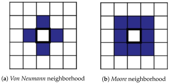
Figure 2.
Patterns of the von Neumann and Moore neighborhood definitions.
The different software systems for landscape analysis use both of these definitions:
- the r.li/r.le modules in GRASS GIS uses the von Neumann definition [55];
- the LecoS plugin for QGIS uses the Moore definition [49];
- FRAGSTATS allows the user to choose between the two definitions [42].
The evaluation of some landscape metrics is influenced by the choice of this parameter. Corner edge cells of the same land use class will be considered part of the same patch in a 8-cells neighborhood, while they are not considered such using a 4-cells neighborhood algorithm.
For this reason, using the same map in different software will lead to different results for some landscape metrics. While LecoS, r.le, and r.li allow the use of one single type of neighbors rule, in FRAGSTATS the default option is the 8-cells Moore definition but the user can select the 4-cells von Neumann one.
3.3. Artificial Maps
Four artificial maps were created to test the sensitivity of the different metrics to the variation of the cell neighborhood value and to understand which patches’ configurations are more susceptible to different values of the cell neighborhood (CN) value. The four maps are binary, with value 1 indicating the patches and value 0 the background. The maps are square, with 100 cell sides, for a total of 10,000 cells and each pixel measures 10 × 10 map units.
The fist map is configured as a chessboard (Figure 3), alternating cells with value 1 and 0. Since each pixel of value 1 represents a separate patch, the total number of patches (NP) is 5000, the patch density (PD), which is maximum for this configuration, is equal to 10,000 (number of patches/100 ha), the (uniform) mean patch size (MPS) is 0.01 (ha), the edge density (ED) is 4000 (m/ha), and the landscape shape index (LSI) is 70.71. This configuration is the one that maximizes the difference of outcomes for the different choices of CN values.
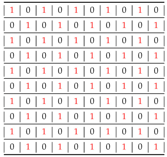
Figure 3.
Scheme of the configuration of the first artificial test map, displayed on a chessboard.
The second map (Figure 4) contains two large patches covering the whole map, separated by a single column of 0 values. For this map the total number of patches (NP) is 2, the patch density (PD) is 2.02 (number of patches/100 ha), the mean patch size (MPS) is 49.5 [ha], the edge density (ED) is 60.4 [m/ha], and the landscape shape index (LSI) is 1.5. The presence of a single edge should result in the same landscape metrics values for both choices of CN.
Figure 4.
Scheme of the configuration of the second artificial test map, consisting of two large patches separated by a single column of 0 values.
The third map (Figure 5) consists in a single, compact, large patch covering half of the map. For this map the total number of patches (NP) is 1, the patch density (PD) is 2 (number of patches/100 ha), the mean patch size (MPS) is 50 (ha), the edge density (ED) is 60 (m/ha) and the landscape shape index (LSI) is 1.06. This configuration is expected to provide the same results for any CN choice, since there is only one edge and the patch is larger than the area corresponding to the largest possible value of CN, 8.
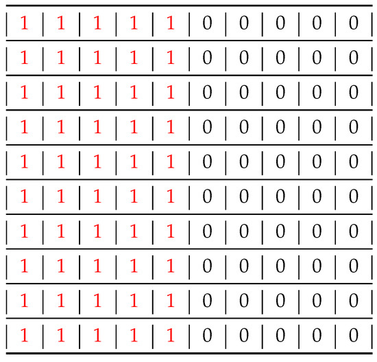
Figure 5.
Scheme of the configuration of the third artificial test map, consisting of a single large patch occupying the left half of the map.
The fourth test map (Figure 6) contains a single patch consisting of just one pixel at the center of the map. For this map the total number of patches (NP) is 1, the patch density (PD) is 10,000 (number of patches/100 ha), the mean patch size (MPS) is 0.01 (ha), the edge density (ED) is 4000 (m/ha) and the landscape shape index (LSI) is 1.
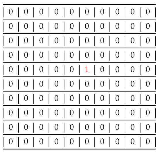
Figure 6.
Scheme of the configuration of the fourth artificial test map, consisting of a single patch of one pixel at the center of the map.
The only cell of value 1 is surrounded by 8 cells of value 0. Therefore, the two choices of CN should yield the same results for the landscape metrics.
3.4. Real Maps
A map of the forest coverage in the Val di Fassa, Italy, in 2006 was used for the tests on real maps. Val di Fassa is a valley in the Alps, in the north east of the Trentino region in Northern Italy (Figure 7). This area was affected by a marked expansion of the forested area in the last century [6,41,51,52] and is currently being investigated in the Trentinoland project, which is analyzing the forest cover of the whole Trentino region in Northern Italy [56].
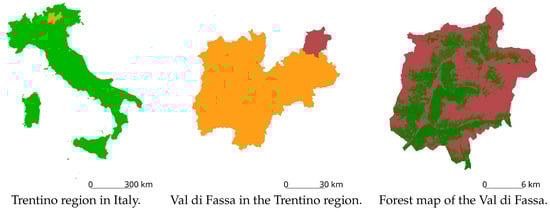
Figure 7.
Location of Trentino region, in orange (in Italy), the Val di Fassa, in red (in the Trentino region), and the forest area in green (in Val di Fassa).
Val di Fassa has an area of 567.28 km (56,728 ha), of which 132.36 km (13,236 ha, 23.33%) were covered by forest in 2006. The region boundaries are 5157094 N, 5132029 S, 721983 E, 699351 W, in the ETRS89/UTM 32 N (EPSG 25832) datum. The raster map has a 10 m resolution, with 2509 rows and 2265 columns, for a total of 5,682,885 cells.
Two maps were derived from this map, by applying a low pass filter with a 3 × 3 pixels window, assigning the third quartile for the first map (Figure 8, center) and the first quartile for the second one (Figure 8, right), with the aim to test how the fragmentation of the maps influences the variation of the landscape metrics depending on the CN value. The application of a low-pass filter obviously leads to less fragmented maps. These maps will be used to develop an index predicting how different values of CN influence landscape metrics values when CN is unknown in Section 5.
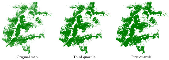
Figure 8.
Maps of the forest coverage of Val di Fassa in 2006, original map (left), filtered with the third quartile (center) and first quartile (right).
These two maps cover the same area and have the same resolution of the original one.
Additionally, three maps representing the forest coverage in 1954, 1974, and 1994 (Figure 9), which present different degrees of fragmentation, have been used to compare the number of patches evaluated using different values of CN.
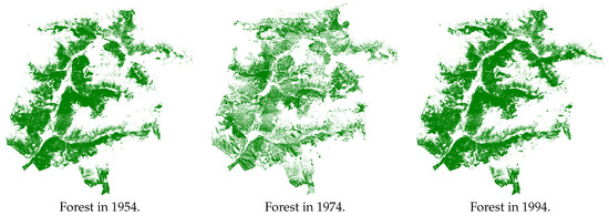
Figure 9.
Forest coverage in Val di Fassa in 1954 (left), 1974 (center), and 1994 (right).
All these maps were created by automatic classification of aerial images using the same classification scheme. An area is considered forest if 20% of the ground area is covered by trees and it is larger than 2000 m with a minimum width of 20 m.
4. Results
For each test map described in Section 3.3 and Section 3.4, the landscape metrics listed in Section 3.2 were evaluated using GRASS GIS, FRAGSTATS, and QGIS. Values for the artificial maps described in Section 3.3 are reported in Table 2, Table 3, Table 4 and Table 5.
Table 2.
Landscape metrics for artificial test map 1 (chessboard).
Table 3.
Landscape metrics for artificial test map 2 (two large patches).
Table 4.
Landscape metrics for artificial test map 3 (a large patch covering half of the map).
Table 5.
Landscape metrics for artificial test map 4 (a single patch of one pixel).
For the first artificial test map (Figure 3), configured as a chessboard, Table 2 shows how a 4-cells CN (GRASS, FRAGSTATS using 4 cells) is able to recognize the 5000 patches corresponding to single pixels and to correctly evaluate the corresponding metrics, while using 8-cells CN (QGIS, FRAGSTATS using 8 cells) one single patch is detected. This difference influences the patch density (PD) and mean patch size (MPS) metrics because they depend on the number of patches. Conversely, edge density (ED) and landscape shape index (LSI) do not change using different CN values because the lengths of all edge segments and the total landscape area change in the same proportion.
Results for the second artificial test map (Figure 4), with two large patches separated by a single straight edge. Table 3 shows how all the landscape metrics values are the same regardless of the value of CN used. This is obviously due to the fact that the map contains only two large compact patches with no fragmentation and a single edge.
For the third artificial test map (Figure 5), with a large patch covering half of the map, Table 4 reports how all the landscape metrics do not change with different CN choices. The reason is the same as for the previous map.
Table 5 shows how both choices for CN correctly detect the only patch, composed by a single pixel, present in the fourth artificial test map (Figure 6). All the landscape metrics values are the same for the different CN values.
Finally, results for the real forest map are reported in Table 6. Values provided by QGIS for mean patch size and edge density differ from those calculated by FRAGSTATS with the same CN value by 4 orders of magnitude, respectively of a factor and . This is due to the fact that areas in QGIS are expressed in square meters, while in GRASS and FRAGSTATS, is used. Therefore, the values of the two mean patch size and edge density metrics for QGIS were rescaled using in Table 6. The same procedure will be applied to all the successive results from QGIS.
Table 6.
Landscape metrics for the 2006 forest map of Val di Fassa, values for QGIS in .
It is evident from Table 6 that some metrics, such as number of patches, patch density, and mean patch size, change when different values of CN are used. Edge density (ED) and landscape shape index (LSI) values are independent from the choice for CN.
5. Aggregation Index
The literature review of Section 2 revealed that in many cases the value of CN is not explicitly stated. Sometimes it is possible to infer the value by the indication of the GIS software used for the processing but even then there can be some ambiguity, such as for the case of FRAGSTATS which can use two different values and the default depends on the software version.
For this reason, it was investigated whether it is possible to find a parameter indicating how the uncertainty on the CN value reflects on the significance of the landscape metrics. Tests on artificial maps (Section 4, Table 2, Table 3, Table 4 and Table 5) showed how the more fragmented a map is the more the values of landscape metrics change for different values of CN. Therefore, the aggregation index (AI), defined in Section 3.2, can be used as an indicator of the importance of the knowledge of CN for the analysis of a map. Its value varies between 0 and 100; it is 0 when the patch class is completely disaggregated, i.e., there are no like adjacencies; it is 100 when the patch class is completely aggregated in a single compact patch. Since tests in Section 3.3 and Section 3.4 have shown that for a given value of CN landscape metrics do not depend on the software used to evaluate them, all the values reported in this section were evaluated using FRAGSTATS.
The first tests to investigate a possible relationship between the AI and the variation of the values of landscape metrics using different CN values were carried out on the artificial maps described in Section 3.3. Table 7 shows the values of the AI for the four artificial maps, the number of patches obtained using values of CN 4 and 8, and their variation as percentage.
Table 7.
Aggregation index and difference in the number of patches using cell neighbourhood (CN) values of 4 and 8 for the 4 artificial maps.
For the first raster, with a chessboard configuration, disaggregation is maximum and the AI is 0, while the difference in the number of patches for the two values of CN is nearly 100%. Conversely, the second and third artificial maps have an AI above 99% and the number of patches does not depend on CN (Table 3 and Table 4). Finally, for the last artificial map the AI is undefined, since it is not possible to evaluate the AI for classes consisting of a single patch. These first tests show (Table 7) that for maps with low values of AI the use of different values of CN leads to large variations of even a simple metric such as the number of patches, while for maps with high AI values the choice for CN becomes irrelevant. The four artificial maps were built to represent extreme configurations; therefore, this hypothesis was tested on real maps. The three maps for the forest in Val di Fassa in 2006, described in Section 3.4, represent a sequence of maps with increasing patch compactness, as shown in Figure 8.
Table 8 reports landscape metrics evaluated using four cells CN and eight cells CN for the three maps. AI values do not depend on the choice of CN; therefore, it can be used to assess the effect of the variation of CN on landscape metrics.
Table 8.
Landscape metrics for the three forest maps of Val di Fassa with 4 cells and 8 cells CN.
Figure 10 shows the variation of the number of patches, patch density, and mean patch size metrics as a function of AI, both in the cases of 4 and 8 cells CN.
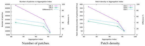
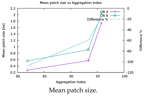
Figure 10.
Variation of number of patches, patch density, and mean patch size landscape metrics as a function of AI for CN values of 4 and 8, left scale, and their difference in percentage, right scale, evaluated on the map representing the forest coverage in Val di Fassa in 2006 and the two maps obtained by applying a low pass filter with a 3 × 3 pixels window, assigning the first and the third quartile.
The difference between values obtained with the two values of CN decreases when the AI increases for all the tested indexes. In fact, the differences for the number of patches and the patch density decrease from 51.6% to 14.0%, while the difference for mean patch size, negative because the mean patch size increases with CN, varies from −107.4% to −16.7% (Table 9).
Table 9.
Differences for number of patches, patch density (PD) (number of patches/100 ha) and mean patch size (MPS) (ha) for the two values of CN (4 or 8 cells) for the map representing the forest coverage in Val di Fassa in 2006 and the two maps obtained by applying a low pass filter with a 3 × 3 pixels window, assigning the first and the third quartile.
These tests show that using a different value for the CN leads to large differences for landscape metrics for fragmented maps, while the metrics values are similar for maps with more aggregated patches. Therefore, the aggregation index can be used as an indicator to assess the suitability of the values of the landscape metrics for making comparisons when the CN value is unknown.
To further test this hypothesis, the number of patches was evaluated for three forest maps of Val di Fassa in 1954, 1974, and 1994 with the two values for CN. The results are reported in Table 10; for these maps the difference of number of patches is higher when the AI is lower.
Table 10.
Differences of number of patches for the two values of CN (4 or 8 cells) for the three forest maps of Val di Fassa in 1954, 1974, and 1994.
For these maps the AI varies from 76.6% to 88.3%, with the difference in number of patches between the two CN values ranging from 47.37% (1994 map) to 59.89% (1974 map).
Figure 11 plots all the couples of values of AI and difference in number of patches using 4 and 8 cells CN in percentage for the six forest maps.
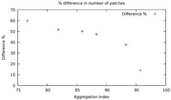
Figure 11.
Difference in number of patches using 4 and 8 cells CN in percentage as a function of AI for the six forest maps.
When AI is lower than 95% the difference in the number of patches ranges from 37% to 60%, while for the highest value the difference is 14%.
6. Conclusions
This study provides an assessment of the importance of the knowledge of the cell neighborhood value when using landscape metrics. Tests on specially crafted maps have shown that CN can affect the values of some metrics with variations up to 5000%. For real maps the variation is not so dramatic but in some cases it can still reach 100% (Table 6). Therefore, the knowledge of the value used for the cell neighborhood (CN) parameter is fundamental, especially if metrics’ values are compared across studies from different research groups using different software, even if the same classification scheme is used. Nevertheless, software users often seem to underestimate the importance of the effects that CN can have on landscape metrics and the selected CN value is often omitted.
When the CN is unknown, tests in Section 5 showed that it is possible to use the values of the aggregation index to assess the effect that the uncertainty on CN can have on some landscape metrics, thus providing an indication of the reliability of comparison with other metrics’ evaluations. The determination of an analytical link between the AI and the significance of CN for landscape metrics evaluation is under way. This could lead to the identification of a threshold AI value below which the knowledge of the CN is essential. From the user perspective, the choice of cell neighborhood is implicit in the choice of the software. A 4-cells CN provides more evident trends for some metrics, see e.g., Figure 10. The main recommendation is to use the same cell neighborhood when comparing results. Moreover, researchers should clearly indicate the CN values when presenting their results.
Supplementary Materials
The following are available online at https://www.mdpi.com/2220-9964/8/12/586/s1.
Author Contributions
Research conceptualization, Paolo Zatelli, Stefano Gobbi, Clara Tattoni and Marco Ciolli; methodology and software Paolo Zatelli, Marco Ciolli, Clara Tattoni and Stefano Gobbi; validation, Paolo Zatelli and Nicola Zorzi, Stefano Gobbi, Clara Tattoni and Marco Ciolli; writing—original draft preparation, Paolo Zatelli, Stefano Gobbi, Clara Tattoni and Marco Ciolli; writing—review and editing, Stefano Gobbi, Marco Ciolli, Nicola La Porta, Duccio Rocchini, Clara Tattoni, Maria Giulia Cantiani and Paolo Zatelli; funding acquisition, Marco Ciolli, Nicola La Porta and Paolo Zatelli.
Funding
Stefano Gobbi is funded by Doctoral Programme in Civil, Environmental and Mechanical Engineering established at the Department of Civil, Environmental and Mechanical Engineering at the University of Trento and Fondazione Edmund Mach.
Conflicts of Interest
The authors declare no conflict of interest.
Abbreviations
The following abbreviations are used in this manuscript:
| AI | aggregation index |
| CN | cell neighborhood |
| ED | edge density |
| GIS | geographic information system |
| GPL | Gnu Public License |
| FOSS | free and open source software |
| LSI | landscape shape index |
| MPS | mean patch size |
| NP | number of patches |
| PD | patch density |
Appendix A. Available Metrics
Feature tables for FRAGSTATS 4.2, GRASS 7.6 (r.li), and QGIS 3.4 (LecoS 3.0.0). Names of metrics change in different software systems, names in the following tables are from the FRAGSTATS 4.2 manual [45].
Table A1.
Software features: cell neighborhood and available area and edge metrics for FRAGSTATS, GRASS (r.li), and QGIS (LecoS).
Table A1.
Software features: cell neighborhood and available area and edge metrics for FRAGSTATS, GRASS (r.li), and QGIS (LecoS).
| FRAGSTATS | GRASS | QGIS | |
|---|---|---|---|
| Cell neighborhood | 4 or 8 cells | 4 cells | 8 cells |
| Patch Metrics | |||
| Patch Area (AREA) | ✓ | ✓ | |
| Patch Perimeter (PERIM) | ✓ | ||
| Radius of Gyration (GYRATE) | ✓ | ||
| Class Metrics | |||
| Total (Class) Area (CA) | ✓ | ✓ | |
| Percentage of Landscape (PLAND) | ✓ | ✓ | ✓ |
| Largest Patch Index (LPI) | ✓ | ||
| Total Edge (TE) | ✓ | ✓ | |
| Edge Density (ED) | ✓ | ✓ | ✓ |
| Patch Area Distribution (AREA_MN, _AM, _MD, _RA, _SD, _CV) | ✓ | ||
| Radius of Gyration Distribution (GYRATE_MN, _AM, _MD, _RA, _SD, _CV) | ✓ | ||
| Landscape Metrics | |||
| Total Area (TA) | ✓ | ✓ | |
| Largest Patch Index (LPI) | ✓ | ✓ | |
| Total Edge (TE) | ✓ | ||
| Edge Density (ED) | ✓ | ✓ | |
| Patch Area Distribution (AREA_MN, _AM, _MD, _RA, _SD, _CV) | ✓ | ✓ | |
| Radius of Gyration Distribution (GYRATE_MN, _AM, _MD, _RA, _SD, _CV) | ✓ | ||
Table A2.
Software features: available shape metrics for FRAGSTATS, GRASS (r.li), and QGIS (LecoS).
Table A2.
Software features: available shape metrics for FRAGSTATS, GRASS (r.li), and QGIS (LecoS).
| FRAGSTATS | GRASS | QGIS | |
|---|---|---|---|
| Patch Metrics | |||
| Perimeter-Area Ratio (PARA) | ✓ | ||
| Shape Index (SHAPE) | ✓ | ✓ | ✓ |
| Fractal Dimension Index (FRAC) | ✓ | ✓ | |
| Related Circumscribing Circle (CIRCLE) | ✓ | ||
| Contiguity Index (CONTIG) | ✓ | ||
| Class Metrics | |||
| Perimeter-Area Fractal Dimension (PAFRAC) | ✓ | ||
| Perimeter-Area Ratio Distribution (PARA_MN, _AM, _MD, _RA, _SD, _CV) | ✓ | ||
| Shape Index Distribution (SHAPE_MN, _AM, _MD, _RA, _SD, _CV) | ✓ | ✓ | |
| Fractal Index Distribution (FRAC_MN, _AM, _MD, _RA, _SD, _CV) | ✓ | ||
| Linearity Index Distribution (LINEAR_MN, _AM, _MD, _RA, _SD, _CV) | ✓ | ||
| Related Circumscribing Square Distribution (SQUARE_MN, _AM, _MD, _RA, _SD, _CV) | ✓ | ||
| Contiguity Index Distribution (CONTIG_MN, _AM, _MD, _RA, _SD, _CV) | ✓ | ||
| Landscape Metrics | |||
| Perimeter-Area Fractal Dimension (PAFRAC) | ✓ | ||
| Perimeter-Area Ratio Distribution (PARA_MN, _AM, _MD, _RA, _SD, _CV) | ✓ | ||
| Shape Index Distribution (SHAPE_MN, _AM, _MD, _RA, _SD, _CV) | ✓ | ✓ | |
| Fractal Index Distribution (FRAC_MN, _AM, _MD, _RA, _SD, _CV) | ✓ | ||
| Linearity Index Distribution (LINEAR_MN, _AM, _MD, _RA, _SD, _CV) | ✓ | ||
| Related Circumscribing Square Distribution (SQUARE_MN, _AM, _MD, _RA, _SD, _CV) | ✓ | ||
| Contiguity Index Distribution (CONTIG_MN, _AM, _MD, _RA, _SD, _CV) | ✓ | ||
Table A3.
Software features: available core area metrics for FRAGSTATS, GRASS (r.li), and QGIS (LecoS).
Table A3.
Software features: available core area metrics for FRAGSTATS, GRASS (r.li), and QGIS (LecoS).
| FRAGSTATS | GRASS | QGIS | |
|---|---|---|---|
| Patch Metrics | |||
| Core Area (CORE) | ✓ | ||
| Number of Core Areas (NCA) | ✓ | ||
| Core Area Index (CAI) | ✓ | ||
| Class Metrics | |||
| Total Core Area (TCA) | ✓ | ✓ | |
| Core Area Percentage of Landscape (CPLAND) | ✓ | ||
| Number of Disjunct Core Areas (NDCA) | ✓ | ||
| Disjunct Core Area Density (DCAD) | ✓ | ||
| Core Area Distribution (CORE_MN, _AM, _MD, _RA, _SD, _CV) | ✓ | ||
| Disjunct Core Area Distribution (DCORE_MN, _AM, _MD, _RA, _SD, _CV) | ✓ | ||
| Core Area Index Distribution (CAI_MN, _AM, _MD, _RA, _SD, _CV) | ✓ | ||
| Landscape Metrics | |||
| Total Core Area (TCA) | ✓ | ||
| Number of Disjunct Core Areas (NDCA) | ✓ | ||
| Disjunct Core Area Density (DCAD) | ✓ | ||
| Core Area Distribution (CORE_MN, _AM, _MD, _RA, _SD, _CV) | ✓ | ||
| Disjunct Core Area Distribution (DCORE_MN, _AM, _MD, _RA, _SD, _CV) | ✓ | ||
| Core Area Index Distribution (CAI_MN, _AM, _MD, _RA, _SD, _CV) | ✓ | ||
Table A4.
Software features: available contrast metrics for FRAGSTATS, GRASS (r.li), and QGIS (LecoS).
Table A4.
Software features: available contrast metrics for FRAGSTATS, GRASS (r.li), and QGIS (LecoS).
| FRAGSTATS | GRASS | QGIS | |
|---|---|---|---|
| Patch Metrics | |||
| Edge Contrast Index (ECON) | ✓ | ||
| Class Metrics | |||
| Contrast-Weighted Edge Density (CWED) | ✓ | ✓ | |
| Total Edge Contrast Index (TECI) | ✓ | ||
| Edge Contrast Index Distribution (ECON_MN, _AM, _MD, _RA, _SD, _CV) | ✓ | ||
| Landscape Metrics | |||
| Contrast-Weighted Edge Density (CWED) | ✓ | ✓ | |
| Total Edge Contrast Index (TECI) | ✓ | ||
| Edge Contrast Index Distribution (ECON_MN, _AM, _MD, _RA, _SD, _CV) | ✓ | ||
Table A5.
Software features: available aggregation metrics for FRAGSTATS, GRASS (r.li), and QGIS (LecoS).
Table A5.
Software features: available aggregation metrics for FRAGSTATS, GRASS (r.li), and QGIS (LecoS).
| FRAGSTATS | GRASS | QGIS | |
|---|---|---|---|
| Patch Metrics | |||
| Euclidean Nearest Neighbor Distance (ENN) | ✓ | ✓ | |
| Proximity Index (PROX) | ✓ | ||
| Similarity Index (SIMI) | ✓ | ||
| Class Metrics | |||
| Interspersion & Juxtaposition Index (IJI) | ✓ | ||
| Percentage of Like Adjacencies (PLADJ) | ✓ | ✓ | |
| Aggregation Index (AI) | ✓ | ||
| Clumpiness Index (CLUMPY) | ✓ | ||
| Landscape Shape Index (LSI) | ✓ | ||
| Normalized Landscape Shape Index (nLSI) | ✓ | ||
| Patch Cohesion Index (COHESION) | ✓ | ✓ | |
| Number of Patches (NP) | ✓ | ✓ | ✓ |
| Patch Density (PD) | ✓ | ✓ | ✓ |
| Landscape Division Index (DIVISION) | ✓ | ✓ | |
| Splitting Index (SPLIT) | ✓ | ✓ | |
| Effective Mesh Size (MESH) | ✓ | ✓ | |
| Euclidean Nearest Neighbor Distance Distribution (ENN_MN, _AM, _MD, _RA, _SD, _CV) | ✓ | ||
| Proximity Index Distribution (PROX_MN, _AM, _MD, _RA, _SD, _CV) | ✓ | ||
| Similarity Index Distribution (SIMI_MN, _AM, _MD, _RA, _SD, _CV) | ✓ | ||
| Connectance (CONNECT) | ✓ | ||
| Landscape Metrics | |||
| Contagion (CONTAG) | ✓ | ||
| Interspersion & Juxtaposition Index (IJI) | ✓ | ||
| Percentage of Like Adjacencies (PLADJ) | ✓ | ||
| Aggregation Index (AI) | ✓ | ||
| Landscape Shape Index (LSI) | ✓ | ||
| Patch Cohesion Index (COHESION) | ✓ | ||
| Number of Patches (NP) | ✓ | ||
| Patch Density (PD) | ✓ | ||
| Landscape Division Index (DIVISION) | ✓ | ||
| Splitting Index (SPLIT) | ✓ | ||
| Effective Mesh Size (MESH) | ✓ | ||
| Euclidean Nearest Neighbor Distance Distribution (ENN_MN, _AM, _MD, _RA, _SD, _CV) | ✓ | ||
| Proximity Index Distribution (PROX_MN, _AM, _MD, _RA, _SD, _CV) | ✓ | ||
| Similarity Index Distribution (SIMI_MN, _AM, _MD, _RA, _SD, _CV) | ✓ | ||
| Connectance (CONNECT) | ✓ | ||
Table A6.
Software features: available diversity indexes for FRAGSTATS, GRASS (r.li), and QGIS (LecoS).
Table A6.
Software features: available diversity indexes for FRAGSTATS, GRASS (r.li), and QGIS (LecoS).
| FRAGSTATS | GRASS | QGIS | |
|---|---|---|---|
| Landscape Metrics | |||
| Patch Richness Density (PRD) | ✓ | ✓ | |
| Relative Patch Richness (RPR) | ✓ | ||
| Shannon’s Diversity Index (SHDI) | ✓ | ✓ | ✓ |
| Simpson’s Diversity Index (SIDI) | ✓ | ✓ | ✓ |
| Modified Simpson’s Diversity Index (MSIDI) | ✓ | ||
| Shannon’s Evenness Index (SHEI) | ✓ | ✓ | |
| Simpson’s Evenness Index (SIEI) | ✓ | ||
| Modified Simpson’s Evenness Index (MSIEI) | ✓ | ||
References
- Steiniger, S.; Hay, G.J. Free and open source geographic information tools for landscape ecology. Ecol. Inform. 2009, 4, 183–195. [Google Scholar] [CrossRef]
- Wang, X.; Blanchet, F.G.; Koper, N. Measuring habitat fragmentation: An evaluation of landscape pattern metrics. Methods Ecol. Evol. 2014, 5, 634–646. Available online: https://besjournals.onlinelibrary.wiley.com/doi/pdf/10.1111/2041-210X.12198 (accessed on 12 September 2019). [CrossRef]
- Cushman, S.; McGarigal, K.; Neel, M. Parsimony in landscape metrics: Strength, universality, and consistency. Ecol. Indic. 2008, 8, 691–703. [Google Scholar] [CrossRef]
- Lustig, A.; Stouffer, D.B.; Doscher, C.; Worner, S.P. Landscape metrics as a framework to measure the effect of landscape structure on the spread of invasive insect species. Landsc. Ecol. 2017, 32, 2311–2325. [Google Scholar] [CrossRef]
- Sertel, E.; Topaloğlu, R.H.; Şallı, B.; Yay Algan, I.; Aksu, G.A. Comparison of Landscape Metrics for Three Different Level Land Cover/Land Use Maps. ISPRS Int. J. Geo-Inf. 2018, 7, 408. [Google Scholar] [CrossRef]
- Uuemaa, E.; Antrop, M.; Roosaare, J.; Marja, R.; Mander, Ü. Landscape Metrics and Indices: An Overview of Their Use in Landscape Research. Living Rev. Landsc. Res. 2009, 3. [Google Scholar] [CrossRef]
- Ferretti, F.; Sboarina, C.; Tattoni, C.; Vitti, A.; Zatelli, P.; Geri, F.; Pompei, E.; Ciolli, M. The 1936 Italian Kingdom Forest Map reviewed: A dataset for landscape and ecological research. Ann. Silvic. Res. 2018, 42, 3–19. [Google Scholar] [CrossRef]
- Smiraglia, D.; Tombolini, I.; Canfora, L.; Bajocco, S.; Perini, L.; Salvati, L. The Latent Relationship Between Soil Vulnerability to Degradation and Land Fragmentation: A Statistical Analysis of Landscape Metrics in Italy, 1960–2010. Environ. Manag. 2019, 64, 154–165. [Google Scholar] [CrossRef]
- Grafius, D.R.; Corstanje, R.; Harris, J.A. Linking ecosystem services, urban form and green space configuration using multivariate landscape metric analysis. Landsc. Ecol. 2018, 33, 557–573. [Google Scholar] [CrossRef]
- Wang, S.; Yang, K.; Yuan, D.; Yu, K.; Su, Y. Temporal-spatial changes about the landscape pattern of water system and their relationship with food and energy in a mega city in China. Ecol. Model. 2019, 401, 75–84. [Google Scholar] [CrossRef]
- Li, H.; Wu, J. Use and misuse of landscape indices. Landsc. Ecol. 2004, 19, 389–399. [Google Scholar] [CrossRef]
- McGarigal, K.; Cushman, S.; Ene, E. FRAGSTATS v4: Spatial Pattern Analysis Program for Categorical and Continuous Maps. Computer Software Program Produced by the Authors at the University of Massachusetts, Amherst. 2012. Available online: http://www.umass.edu/landeco/research/fragstats/fragstats.html (accessed on 12 September 2019).
- Cushman, S.; States, U.; Service, F.; Mount, R. Behavior of class-level landscape metrics across gradients of class aggregation and area. Landsc. Ecol. 2015, 435–455. [Google Scholar] [CrossRef]
- Saura, S.; Castro, S. Scaling functions for landscape pattern metrics derived from remotely sensed data: Are their subpixel estimates really accurate? ISPRS J. Photogramm. Remote Sens. 2007, 62, 201–216. [Google Scholar] [CrossRef]
- Tanner, E.P.; Fuhlendorf, S.D. Impact of an agri-environmental scheme on landscape patterns. Ecol. Indic. 2018, 85, 956–965. [Google Scholar] [CrossRef]
- Gong, J.-Z.; Liu, Y.-S.; Xia, B.-C.; Zhao, G.-W. Urban ecological security assessment and forecasting, based on a cellular automata model: A case study of Guangzhou, China. Ecol. Model. 2009, 220, 3612–3620. [Google Scholar] [CrossRef]
- Abadie, A.; Gobert, S.; Bonacorsi, M.; Lejeune, P.; Pergent, G.; Pergent-Martini, C. Marine space ecology and seagrasses. Does patch type matter in Posidonia oceanica seascapes? Ecol. Indic. 2015, 57, 435–446. [Google Scholar] [CrossRef]
- Lausch, A.; Herzog, F. Applicability of landscape metrics for the monitoring of landscape change: Issues of scale, resolution and interpretability. Ecol. Indic. 2002, 2, 3–15. [Google Scholar] [CrossRef]
- Ramesh, T.; Kalle, R.; Downs, C.T. Sex-specific indicators of landscape use by servals: Consequences of living in fragmented landscapes. Ecol. Indic. 2015, 52, 8–15. [Google Scholar] [CrossRef]
- Lustig, A.; Stouffer, D.B.; Roigé, M.; Worner, S.P. Towards more predictable and consistent landscape metrics across spatial scales. Ecol. Indic. 2015, 57, 11–21. [Google Scholar] [CrossRef]
- Shen, W.; Jenerette, G.D.; Wu, J.; Gardner, R.H. Evaluating empirical scaling relations of pattern metrics with simulated landscapes. Ecography 2004, 27, 459–469. [Google Scholar] [CrossRef]
- László, Z.; Dénes, A.L.; Király, L.; Tóthmérész, B. Biased parasitoid sex ratios: Wolbachia, functional traits, local and landscape effects. Basic Appl. Ecol. 2018, 31, 61–71. [Google Scholar] [CrossRef]
- Bueno, A.S.; Peres, C.A. Patch-scale biodiversity retention in fragmented landscapes: Reconciling the habitat amount hypothesis with the island biogeography theory. J. Biogeogr. 2019, 46, 621–632. [Google Scholar] [CrossRef]
- Cordeiro, E.M.; Macrini, C.M.; Sujii, P.S.; Schwarcz, K.D.; Pinheiro, J.B.; Rodrigues, R.R.; Brancalion, P.H.; Zucchi, M.I. Diversity, genetic structure, and population genomics of the tropical tree Centrolobium tomentosum in remnant and restored Atlantic forests. Conserv. Genet. 2019, 20, 1073–1085. [Google Scholar] [CrossRef]
- Hernández-Martínez, J.; Morales-Malacara, J.B.; Alvarez-Anõrve, M.Y.; Amador-Hernández, S.; Oyama, K.; Avila-Cabadilla, L.D. Drivers potentially influencing host-bat fly interactions in anthropogenic neotropical landscapes at different spatial scales. Parasitology 2019, 146, 74–88. [Google Scholar] [CrossRef] [PubMed]
- Dennis, M.; Scaletta, K.L.; James, P. Evaluating urban environmental and ecological landscape characteristics as a function of land-sharing-sparing, urbanity and scale. PLoS ONE 2019, 14, e0215796. [Google Scholar] [CrossRef] [PubMed]
- Kurta, A.; Auteri, G.G.; Hofmann, J.E.; Mengelkoch, J.M.; White, J.P.; Whitaker, J.O.; Cooley, T.; Melotti, J. Influence of a large lake on thewinter range of a small mammal: Lake Michigan and the silver-haired bat (Lasionycteris noctivagans). Diversity 2018, 10, 24. [Google Scholar] [CrossRef]
- Kosicki, J.Z. Are Landscape Configuration Metrics Worth Including When Predicting Specialist and Generalist Bird Species Density? A Case of the Generalised Additive Model Approach. Environ. Model. Assess. 2018, 23, 193–202. [Google Scholar] [CrossRef]
- Lamamy, C.; Bombieri, G.; Zarzo-Arias, A.; González-Bernardo, E.; Penteriani, V. Can landscape characteristics help explain the different trends of Cantabrian brown bear subpopulations? Mammal Res. 2019, 559–567. [Google Scholar] [CrossRef]
- Ramachandran, R.M.; Roy, P.S.; Chakravarthi, V.; Sanjay, J.; Joshi, P.K. Long-term land use and land cover changes (1920–2015) in Eastern Ghats, India: Pattern of dynamics and challenges in plant species conservation. Ecol. Indic. 2018, 85, 21–36. [Google Scholar] [CrossRef]
- Monti, F.; Nelli, L.; Catoni, C.; Dell’Omo, G. Nest box selection and reproduction of European Rollers in Central Italy: A 7-year study. Avian Res. 2019, 10, 1–12. [Google Scholar] [CrossRef]
- Morales-Díaz, S.P.; Alvarez-Añorve, M.Y.; Zamora-Espinoza, M.E.; Dirzo, R.; Oyama, K.; Avila-Cabadilla, L.D. Rodent community responses to vegetation and landscape changes in early successional stages of tropical dry forest. For. Ecol. Manag. 2019, 433, 633–644. [Google Scholar] [CrossRef]
- Lastrucci, L.; Cerri, M.; Coppi, A.; Dell’Olmo, L.; Ferranti, F.; Ferri, V.; Filipponi, F.; Foggi, B.; Galardini, R.; Reale, L.; et al. Spatial landscape patterns and trends of declining reed-beds in peninsular Italy. Plant Biosyst. 2019, 153, 427–435. [Google Scholar] [CrossRef]
- Statuto, D.; Cillis, G.; Picuno, P. GIS-based Analysis of Temporal Evolution of Rural Landscape: A Case Study in Southern Italy. Nat. Resour. Res. 2019, 28, 61–75. [Google Scholar] [CrossRef]
- Colson, F.; Bogaert, J.; Filho, A.C.; Nelson, B.; Pinagé, E.R.; Ceulemans, R. The influence of forest definition on landscape fragmentation assessment in Rondônia, Brazil. Ecol. Indic. 2009, 9, 1163–1168. [Google Scholar] [CrossRef]
- Aguilar, R.; Calviño, A.; Ashworth, L.; Aguirre-Acosta, N.; Carbone, L.M.; Albrieu-Llinás, G.; Nolasco, M.; Ghilardi, A.; Cagnolo, L. Unprecedented plant species loss after a decade in fragmented subtropical chaco serrano forests. PLoS ONE 2018, 13, 1–15. [Google Scholar] [CrossRef]
- Albrieu-Llinás, G.; Espinosa, M.O.; Quaglia, A.; Abril, M.; Scavuzzo, C.M. Urban environmental clustering to assess the spatial dynamics of Aedes aegypti breeding sites. Geospat. Health 2018, 13, 135–142. [Google Scholar] [CrossRef]
- Colson, F.; Bogaert, J.; Ceulemans, R. Fragmentation in the Legal Amazon, Brazil: Can landscape metrics indicate agricultural policy differences? Ecol. Indic. 2011, 11, 1467–1471. [Google Scholar] [CrossRef]
- Gaucherel, C.; Burel, F.; Baudry, J. Multiscale and surface pattern analysis of the effect of landscape pattern on carabid beetles distribution. Ecol. Indic. 2007, 7, 598–609. [Google Scholar] [CrossRef]
- Llauss, A.; Nogué, J. Indicators of landscape fragmentation: The case for combining ecological indices and the perceptive approach. Ecol. Indic. 2012, 15, 85–91. [Google Scholar] [CrossRef]
- Tattoni, C.; Ciolli, M.; Ferretti, F. The fate of priority areas for conservation in protected areas: A fine-scale markov chain approach. Environ. Manag. 2011, 47, 263–278. [Google Scholar] [CrossRef]
- McGarigal, K.; Marks, B.J. FRAGSTATS: Spatial Pattern Analysis Program for Quantifying Landscape Structure; USDA For. Serv. Gen. Tech. Rep. PNW-351; U.S. Department of Agriculture, Forest Service, Pacific Northwest Research Station: Portland, OR, USA, 1995.
- GRASS Development Team. Geographic Resources Analysis Support System (GRASS) Software. Open Source Geospatial Foundation. 2017. Available online: grass.osgeo.org (accessed on 12 September 2019).
- QGIS Development Team. QGIS Geographic Information System. Open Source Geospatial Foundation Project. 2019. Available online: http://qgis.osgeo.org (accessed on 12 September 2019).
- McGarigal, K. FRAGSTATS HELP. 2015. Available online: https://www.umass.edu/landeco/research/fragstats/documents/fragstats.help.4.2.pdf (accessed on 12 September 2019).
- Neteler, M.; Bowman, M.; Landa, M.; Metz, M. GRASS GIS: A multi-purpose Open Source GIS. Environ. Model. Softw. 2012, 31, 124–130. [Google Scholar] [CrossRef]
- Ciolli, M.; Federici, B.; Ferrando, I.; Marzocchi, R.; Sguerso, D.; Tattoni, C.; Vitti, A.; Zatelli, P. FOSS tools and applications for education in geospatial sciences. ISPRS Int. J. Geo-Inf. 2017, 6, 225. [Google Scholar] [CrossRef]
- GRASS Development Team. GRASS GIS Performance. 2019. Available online: https://grasswiki.osgeo.org/wiki/GRASS_GIS_Performance (accessed on 15 September 2019).
- Jung, M. LecoS—A python plugin for automated landscape ecology analysis. Ecol. Inform. 2016, 31, 18–21. [Google Scholar] [CrossRef]
- Zaragozí, B.; Belda, A.; Linares, J.; Martínez-Pérez, J.E.; Navarro, J.T.; Esparza, J. A Free and Open Source Programming Library for Landscape Metrics Calculations. Environ. Model. Softw. 2012, 31, 131–140. [Google Scholar] [CrossRef]
- Hesselbarth, M.H.K.; Sciaini, M.; With, K.A.; Wiegand, K.; Nowosad, J. landscapemetrics: An open-source R tool to calculate landscape metrics. Ecography 2019, 42, 1648–1657. [Google Scholar] [CrossRef]
- Ciolli, M.; Tattoni, C.; Ferretti, F. Understanding forest changes to support planning: A fine-scale Markov chain approach. Dev. Environ. Model. 2012, 25, 355–373. [Google Scholar] [CrossRef]
- Tattoni, C.; Ciolli, M.; Ferretti, F.; Cantiani, M.G. Monitoring spatial and temporal pattern of Paneveggio forest (Northern Italy) from 1859 to 2006. IForest 2010, 3, 72–80. [Google Scholar] [CrossRef]
- McGarigal, K. Landscape Pattern Metrics. In Wiley StatsRef: Statistics Reference Online; American Cancer Society: New York, NY, USA, 2014; Available online: https://onlinelibrary.wiley.com/doi/pdf/10.1002/9781118445112.stat07723 (accessed on 12 September 2019). [CrossRef]
- Baker, W.; Cai, Y. The r.le programs for multiscale analysis of landscape structure using the GRASS geographical information system. Landsc. Ecol. 1992, 7, 291–302. [Google Scholar] [CrossRef]
- Gobbi, S.; Cantiani, M.G.; Rocchini, D.; Zatelli, P.; Tattoni, C.; Ciolli, M.; La Porta, N. Fine spatial scale modelling of Trentino past forest landscape (Trentinoland): A case study of FOSS application. In Proceedings of the International Archives of the Photogrammetry, Remote Sensing and Spatial Information Sciences—ISPRS Archives, Bucharest, Romania, 26–30 August 2019; Volume XLII-4/W14, pp. 71–78. [Google Scholar] [CrossRef]
© 2019 by the authors. Licensee MDPI, Basel, Switzerland. This article is an open access article distributed under the terms and conditions of the Creative Commons Attribution (CC BY) license (http://creativecommons.org/licenses/by/4.0/).